Numerical investigation of spatially nonhomogeneous acoustic agglomeration using sectional algorithm

Abstract

In the simulation of acoustic agglomeration, the conventional temporal model assumes spatial homogeneity in aerosol properties and sound field, which is often not the case in real applications. In this article, we investigated the effects of spatial nonhomogeneity of sound field on the acoustic agglomeration process through a one-dimensional spatial sectional model. The spatial sectional model is validated against existing experimental data and results indicate lower requirements on the number of sections and better accuracy. Two typical cases of spatial nonhomogeneous acoustic agglomeration are studied by the established model. The first case involves acoustic agglomeration in a standing wave field with spatial alternation of acoustic kernels from nodes to antinodes. The good agreement between the simulation and experiments demonstrates the predictive capability of the present spatial sectional model for the standing-conditioned agglomeration. The second case incorporates sound attenuation in the particulate medium into acoustic agglomeration. Results indicate that sound attenuation can influence acoustic agglomeration significantly, particularly at high frequencies, and neglecting the effects of sound attenuation can cause overprediction of agglomeration rates. The present investigation demonstrates that the spatial sectional method is capable of simulating the spatially nonhomogeneous acoustic agglomeration with high computation efficiency and numerical robustness and the coupling with flow dynamics will be the goal of future work.

Copyright © 2018 American Association for Aerosol Research

EDITOR:

• Nicole Riemer

1. Introduction

In recent years, particles of microns and submicrons diameter are gaining attention as being harmful to public health (Pope et al. 2000). To effectively remove particles from the air, the particle removal technologies such as electrostatic precipitators, filters, cyclones, and scrubbers are often used (Lee and Liu 1981; Kim and Lee 1990; Bush and Snyder 1992). However, Riley et al. (2002) reported that a major challenge of the current particle removal technologies is the poor efficiency for small particles such as PM2.5 (particulate matter with a diameter of less than 2.5 µm). Acoustic agglomeration, as a preconditioning technique, is a process in which small particles in a suspension collide with one another to form large agglomerates under the action of a sound field. As a result, particle size distribution can shift significantly to a range of larger particulates within a short period of time, and the efficiency of conventional particle removal technologies is greatly improved (Lee et al. 1981; Sarabia et al. 1986; Malherbe et al. 1988; Caperan et al. 1995; Gallego-Juarez et al. 1999; Yuen et al. 2014; Ma et al. 2017; Ng et al. 2017).

Numerical simulation has been widely employed as a convenient and economic way to investigate the phenomena of acoustic agglomeration and to optimize the experimental conditions (Tiwary and Reethof 1987; Song 1990; Ezekoye and Wibowo 1999; Sheng and Shen 2006, 2007; Fan et al. 2017). In the simulation, the aerosol and sound field are often assumed to be homogeneous within the geometric boundaries. Under these circumstances, the particle size distribution function n(v,t) is only dependent on the time t and the particle volume v, and governed by a temporal model. The temporal evolution of the aerosol with acoustic agglomeration can be described by the Smoluchowski equation (Friedlander 2000) (1) where is the agglomeration kernel in the acoustic agglomeration process. The Smoluchowski equation is a partial, non-linear, and integro-differential equation that has only a limited number of known analytical solutions. As such, numerical simulations are often conducted to obtain approximate solutions to investigate the acoustic agglomeration process. Tiwary and Reethof (1987) developed a numerical scheme to solve the temporal model Equation (1)(1) and simulated the acoustic agglomeration of fly ashes in a travelling wave field. The simulation gave reasonable prediction of the agglomeration rates and particle size distribution (PSD) against experimental results for 140–160 dB sound pressure level (SPL). For a higher SPL of 160 dB, discrepancies between simulations and experiments were reported when the exposure time was 6 s or more. Another method to resolve the aerosol dynamic equation is through the use of the direct simulation Monte Carlo (DSMC) method. This was demonstrated by Sheng and Shen where the agglomeration of spherical and fractal particles in a travelling wave field was simulated (Sheng and Shen 2006, 2007). It was observed that limitations exist in the acoustic kernels in covering a broad range of experimental conditions and further efforts were suggested to improve the simulation of acoustic agglomeration. The sectional algorithm, first proposed by Gelbard and Seinfeld (1980), has been extensively used in the simulation of aerosol dynamics. This method divides the continuous particle size distribution into discrete sections and in each section, the PSD can be regarded as uniform or any pre-defined function. Using the sectional method to solve the temporal model Equation (1)(1) , Ezekoye and Wibowo (1999) compared their computation results with experimental measurements and results showed that the temporal sectional model can predict the trends of the aerosol evolution but greatly overpredicts the agglomeration rates.

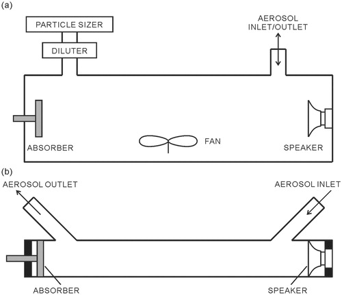
The temporal model assumes that all the properties of the aerosol and sound field are homogeneous within the geometry without spatial variation of any quantity involved in the acoustic agglomeration process. Specifically, homogeneity requires that both the concentration and the particle distribution are identical everywhere in the chamber and the sound field is travelling wave field with negligible attenuation along the propagation length. This restricts the temporal model in its application to the agglomerator shown in Figure 1a, which involves homogeneous particle size distribution and insignificantly attenuated travelling fields. In typical experimental set-ups, fans are often used for particle mixing and the inlet/outlet valve is turned off during the acoustic agglomeration process. However, in industrial engineering or laboratory experiments, it is often encountered that the aerosol particles within the acoustic domain move in a mean flow as shown in Figure 1b. Under such situation, it is necessary to investigate the spatial evolution of the aerosol inside the agglomerator under given operating conditions (e.g., the sound frequency, SPL, and temperature etc.) in the numerical simulation of acoustic agglomeration. Besides, the acoustic fields themselves are not spatially homogenous, rendering the assumptions that any properties of the aerosol and sound field are uniform in space in the temporal model invalid. For example, in a standing wave field, the acoustic velocity amplitude displays node-antinode alternations in the propagation direction, which itself commands varying acoustic kernels to represent spatial differences in particle agglomerations. However, the conventional temporal model supposes that the acoustic kernels are equal along the propagation direction, which causes considerable deviation between the experimental and simulation results (Sarabia et al. 2003). In addition, researchers have demonstrated that it is usual for the SPL to vary by 3–5 dB along the length of the agglomeration chamber due to particulate medium interactions (Ezekoye and Wibowo 1999). In fact, a drop in SPL of 3 dB corresponds to a factor of two in terms of the reduction in acoustic velocity, which means that the attenuation of sound fields in acoustic agglomeration is considerable. Hence, to overcome limitations in the current temporal model, a spatial aerosol dynamical model is required for the prediction of acoustic agglomeration under spatially nonhomogeneous aerosol properties and sound fields.

Figure 1. Illustration of the acoustic agglomerator: (a) homogeneous; (b) nonhomogeneous.

Compared to the extensive numerical simulations of the temporal model, only a limited number of studies have been reported to investigate the spatial acoustic agglomeration. Zhao and Zheng (2013) developed a differentially-weighted Monte Carlo method to solve the population balance equation. In their simulation, the time step is required to be extremely small, and the tracking of individual particles is computationally complicated. Fan et al. (2017) adopted this method to simulate a typical case of acoustic agglomeration with only 7650 particles, but the computation time was up to 4 days on a computer equipped with 4 CPUs (Intel i5) and RAM of 8192 MB. Song (1990) developed a numerical algorithm based on discrete size bins, and simulated the steady-state and one-dimensional acoustic agglomeration of fly ashes under various operating conditions. However, Song’s method is a coarse approximation of the sectional algorithm and requires a large number of size bins, leading to enormous computation times and memory usage. Therefore, it remains to be a great challenge to simulate the spatially nonhomogeneous acoustic agglomeration with economic time and memory consumption.

In the present study, sectional algorithm is applied to simulate spatially nonhomogeneous acoustic agglomeration with variation of aerosol properties and sound fields in space. The discrete formulation of the aerosol dynamic equation, which incorporates the convective transport of aerosols, is constructed based on the sectional approach and the acoustic agglomeration kernel is presented as a source term in the equation. To demonstrate the capability of the proposed spatial sectional model, a simplified analysis of a one-dimensional model is carried out to study the effects of spatial non-uniformity on acoustic agglomeration under two typical circumstances: acoustic agglomeration in a standing wave field and attenuated acoustic agglomeration in a travelling wave field.

2. Modelling

2.1. Sectional formulation of the tempo-spatial general dynamic equation

The tempo-spatial evolution of particle size distribution in aerosol dynamics is governed by the general dynamic equation (GDE, Friedlander 2000) (2) where the particle size distribution function n or n() is dependent on the space vector , time t, and the particle volume v. The terms U and U_ext are the velocity of particles due to convective transport and external forces, respectively, and D is the diffusion coefficient. In acoustic agglomeration, the high-order acoustic effects, such as acoustic radiation and acoustic streaming, can induce a drifting velocity of particles and increase the probability of particle collision and agglomeration (Yuen et al. 2014, 2016, 2017). Additionally, the acoustic radiation force and acoustic streaming can enhance the impaction of particles onto the boundary surfaces and as a result encourage the particle deposition (Yuen et al. 2014). To significantly influence the acoustic agglomeration, the high-order acoustic effects usually need to operate at ultrasound frequencies. In the present study, to avoid complications and focus on the effects of spatial nonhomogeneity, we restricted the typical frequency for acoustic agglomeration below ultrasound. Within this frequency range, the contribution of the high-order effects to acoustic agglomeration would be relatively small compared to the first-order acoustic velocity in either travelling or standing wave conditions. As such, the high-order acoustic effects can be neglected in the simulation (Riera et al. 2015). Therefore, for the process containing acoustic agglomeration only, the GDE can be written as (3) where the source term of the aerosol particles due to acoustic agglomeration is expressed by (4) which represents the size distribution of particles at any location and time under the transport processes of diffusion, convection, and acoustic agglomeration. In acoustic agglomeration, both the aerosol properties (PSD and concentration) and flow characteristics (transport velocity) fluctuate periodically with time around their average values. This results in the variables found in Equation (3)(3) consisting of two components: the mean value and the fluctuation during each period of acoustic cycle. It is assumed that the fluctuations are much smaller than their mean values and the integrations of the fluctuation terms over one period are equal to zero. When neglecting the higher order terms, we can also use Equation (3)(3) to describe the first-order equation of the mean values for all the variables which overlook the periodic fluctuation within one acoustic cycle. Additionally, with the sampling time of typical aerosol measurement instruments in the order of several seconds (accounts for thousands of acoustic cycles), the periodic fluctuations will be filtered out in experimental measurements.

Following the notation of Gelbard and Seinfeld (1980), a general property of the aerosol is introduced as (5) where α and γ are constants that determine the general property of an aerosol (number, volume, or surface area concentration etc.).

Dividing the entire particle size domain into a finite number of sections, one can define a discrete quantity of the aerosol in the l-th section as (6) where, for α = 1 and γ = 0, is the particle number concentration, N_l, while for α = 1, γ = 1, is the particle volume concentration, V_l.

By applying Equation (6)(6) to the general dynamic Equation (3)(3) , the sectional formulation for a general quantity of the aerosol in the l-th section can be written as follows: (7)

The sectional source term in the l-th section, S_l, which results from the agglomeration process, is written as (8) where NS is the number of sections and the sectional kernels, , , _, and , represent the inter- and intra-sectional agglomeration coefficients between sections prior to the l-th section, the agglomeration between the l-th section and lower sections, agglomeration within the l-th section, and agglomeration between the l-th section and higher sections, respectively. The detailed derivation of the sectional kernels is demonstrated in the online supplementary information (SI).

In most industrial applications, the operating conditions, for example, the sound frequency, SPL, or PSD at the inlet, do not vary with time. Hence, the mean values of all the variables over one cycle are independent on time, and the agglomeration process after averaging over one acoustic cycle can be regarded as steady state provided that all the periodic fluctuations within each acoustic cycle are neglected. Furthermore, a typical acoustic agglomerator works at the Reynolds number (Re) ranging from 5000 to 10⁵, indicating that the air stream is turbulent (Ezekoye and Wibowo 1999; Riera et al. 2015). The turbulent diffusion of particles can be several orders of magnitude more intense than Brownian diffusion due to the strong velocity fluctuations. However, according to Sheriff and O’Kane (1971), the turbulent diffusivity is smaller than 10⁻² m²/s under the flow conditions of 5000 < Re < 10⁵ and as a result the Peclet number (Pe) is much greater than unity, Pe ≫ 1. Peclet number describes the relative importance of the convection to the diffusion in mass transfer and thus, the dominant particle transport mechanism is convection inside a typical acoustic agglomerator and the diffusion term can be safely neglected. In the present study, a simplified one-dimension model is analyzed by assuming that all the variables are varied in the direction of fluid flow only. Under such circumstances, one obtains the sectional one-dimensional aerosol dynamic equation (9) where U_x is the mean velocity of the flow, Q_l can be any general integral quantity of the aerosol, such as the number concentration N_l, surface area S_l, volume concentration V_l, or mass concentration M_l, and correspondingly, the sectional kernels have different expressions as shown in the online SI. For each time step, the source terms are first calculated from the space-dependent kernels, and the sectional Equation (9)(9) is then solved by marching technique for all the sections.

2.2. Acoustic kernels

The acoustic kernel is the volume rate of particle agglomeration in a specified volume, which quantifies the effect of acoustic fields on the agglomeration process. To derive the acoustic kernel, a variety of mechanisms have been proposed for the interaction between the sound field and suspended particles in aerosols and among them, two primary mechanisms are generally accepted, which are the so-called orthokinetic and hydrodynamic interactions (Mednikov 1965; Song 1990; Hoffmann 1997; Riera et al. 2015).

The orthokinetic mechanism, which was first proposed by Mednikov (1965), results from differences in acoustic entrainment of particles in a carrier medium. Under the oscillation of the carrier medium in a sound field, small particles tend to be entrained more easily than larger particles. As a result, large particles can “collect” small ones due to the relative motions. Assuming that all the small particles in the agglomeration volume are collected by the large particle and refilling efficiency is unity for every acoustic cycle, Mednikov derived the orthokinetic agglomeration kernel as (10) where U_g is the acoustic velocity of the air and η₁₂ is the real part of the entrainment factor . The entrainment function H is calculated by (11)

In the above expression, ω is the angular frequency and τ_d is the dynamic relaxation time of the particle, given by (12) where ρ_p and d_p are the density and diameter of the particle, respectively, and μ is the dynamic viscosity of the air.

However, the orthokinetic mechanism fails to interpret the rapid agglomeration of particles of the same size in acoustic fields, where entrainment velocities among particles are equivalent without relative motions (Shaw and Tu 1979). As such, the hydrodynamic mechanism was proposed to account for monodisperse aerosol agglomeration. Based on Bernoulli’s hydrodynamic principles, there is a net pressure force to draw two particles to approach each other. Konig derived this hydrodynamic force by studying the force between two entrained particles (Riera et al. 2015). Later, by incorporating the mutual scattering interaction and radiation pressure interaction between two particles in an acoustic field, Song (1990) modified the hydrodynamic acoustic agglomeration kernel based on Konig’s and demonstrated that the hydrodynamic interaction is comparable to the orthokinetic interaction, particularly for large particles and high sound frequencies. The hydrodynamic agglomeration kernel modified by Song is written as (13) where ρ_g is the air density and g₁₂ is called the hydrodynamic interaction function, which are given in Song (1990).

When Knudsen number (Kn) is much smaller than 1, the Brownian motion of particles enter continuum regime, and the agglomeration kernel for Brownian diffusion of two particles with the volume v and is given by (Sitarski and Seinfeld 1977) (14) where k_B is the Boltzmann constant, T is the temperature, and μ is the air viscosity.

A comparison between the orthokinetic kernel (solid line), hydrodynamic kernel (dashed line), and Brownian kernel (dot-dashed line) under the ambient conditions is shown in Figure 2. The diameter of particle 1 is 10 µm and the diameter of particle 2 ranges from 0.1 µm to 100 µm. The frequency and SPL are 1500 Hz and 150 dB, respectively. It is shown that the orthorkinetic kernel is relatively constant as the particle diameter ratio is increased. Except when the two particles have analogous sizes, the orthorkinetic kernel takes a dip due to same entrainment velocities of the particles. On the other hand, the hydrodynamic mechanism has an almost linear growth as the size of particle 2 is increased. When the particle 2 is less than 1 µm, the orthokinetic mechanism is dominant, and when the particle diameter ratio increases beyond unity, the hydrodynamic interaction dominates. The acoustic kernels for orthokinetic and hydrodynamic mechanism are of the order of 10⁻⁴ cm³/s or higher, which are much larger than the Brownian kernel (10⁻⁹–10⁻⁸ cm³/s). As such, only the acoustic kernels are considered in the present study, which is described by the additive combination of Mednikov’s kernel – Equation (10)(10) for the orthokinetic interaction and Song’s hydrodynamic kernel – Equation (13)(13) for hydrodynamic interaction. This was the same combination of kernels, which was previously adopted by Ezekoye and Wibowo (1999) in the temporal sectional model.

Figure 2. The orthorkinetic (solid), hydrodynamic (dashed), and Brownian (dot-dashed) kernels with respect to the particle size ratio.

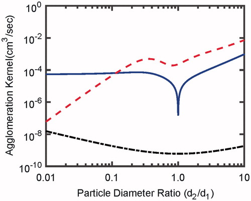
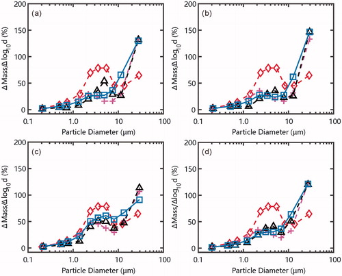
Figure 3. Predictions of the present sectional model (square) compared with the experimental (triangle) and simulation (plus) from Song (1990) for four tests: (a) for HTHP-1, (b) for HTHP-2, (c) for HTHP-3, and (d) for HTHP-4. The initial distribution (diamond) of the aerosol at the chamber inlet is also included.

3. Results and discussion

3.1. Comparison to Song’s algorithm

The prediction of acoustic agglomeration using the present model is compared against the experimental and numerical results of Song (1990). To demonstrate the improvement of the present model compared to Song’s model, the applied sound field is a travelling wave field with constant amplitude, which is the same as that in Song’s simulation. The aerosol considered is fly ash with the density of 2300 kg/m³. The acoustic agglomeration chamber is a cylindrical tube of 2.74 m (9′) in length and 0.15 m (6″) in inner diameter. The operating conditions are set close to the combustion gases from a power plant with high temperature (above 1000 K) and pressure (around 10 bars). Four typical tests are modeled and the operating parameters for each test are listed in Table 1. Assuming the air as an ideal gas, the density, viscosity of the air, and the speed of sound are expressed in terms of the temperature T and pressure P (15) (16) (17) where R = 287 J/(kg·K), κ = 1.4 and µ₀ = 1.71 10⁻⁵ Pa s are the gas constant, specific heat ratio and reference viscosity, respectively. The average flow velocity is calculated from the chamber length and residence time. The spatial sectional Equation (9)(9) is solved for mass concentration M_l and the total number of sections for all tests is chosen to be 11 for computational efficiency.

Table 1. Parameters of tests in Song’s acoustic agglomeration experiments.

Test#	Temperature	Pressure	Mass loading	Residence TIME	SPL	Frequency	Error	Error
	(K)	(kPa)	(g/m^3)	(s)	(dB)	(Hz)	(Song)	(Present)
HTHP-1	810.9	785.4	14.5	4.0	155	900	18.2%	13.6%
HTHP-2	955.4	896.3	15.8	3.8	157	820	12.3%	9.4%
HTHP-3	1060.9	896.3	9.3	3.6	152	910	8.4%	7.3%
HTHP-4	999.8	896.3	17.4	3.5	155	905	9.2%	4.7%

The mass fraction distributions at the outlet of the agglomeration chamber predicted by the present spatial sectional model (square) and through Song’s algorithm (plus) are demonstrated for four tests: (a) for HTHP-1, (b) for HTHP-2, (c) for HTHP-3, and (d) for HTHP-4. The predictions of both models are able to capture the experimental results (triangle) under the same initial conditions for particle distribution (diamond), which verifies the accuracy of the spatial sectional algorithm and computation codes. As a result of particle agglomeration, particle size distribution of the aerosol at the outlet of the acoustic chamber changes with the portion of small particles decreasing and portion of large particles increasing. Furthermore, the average relative error of all sections for the present simulation is compared with that for Song’s simulation by regarding the experimental data as the exact value. As listed in Table 1, the current spatial sectional model shows analogous or even better agreement with the experimental measurements as compared to Song’s numerical results. This is achieved through much smaller number of sections (11 sections) than Song’s simulations (80 size bins) that greatly alleviates the consumption of computation time and memory storage.

In Song’s numerical scheme, the discretized aerosol dynamic equation (or the governing equation) for the k-th size bin (or section) is expressed by (18) where u_p, NS, N, and β_ij are the convective velocity, number of size bins, number concentration, and discretized agglomeration kernel, respectively. A_ijk is the agglomeration redistribution factor, which is detailed in Song (1990). In Song’s algorithm, the discretized agglomeration kernel in each size bin is calculated simply by the acoustic kernel for the average diameter in this size bin (19) where and are the arithmetic average size in the i-th and j-th bin, respectively. It can be seen that the expressions of the numerical equation in Equation (18)(18) and discretized kernel in Equation (19)(19) are different from those in Equations (7)(7) and (8)(8) for the present model, which arises from the difference of the numerical schemes.

The kernel in Equation (19)(19) represents “birth rate” of particles in a size bin resulting from agglomeration between the i-th and j-th size bin. However, the acoustic kernel for either orthokinetic or hydrodynamic interaction is varied with the particle size as shown in Figure 2, and the coarse approximation in Equation (19)(19) gives rise to major computation errors. In the present sectional algorithm, the four agglomeration coefficients for each section are calculated by integrating the acoustic kernels over the particle size in the section as detailed in the online SI, and the variation of the acoustic kernel within each section is taken into account. In addition, Equation (18)(18) can only solve the number concentration of the aerosol and all the other quantities, such as surface area concentration or volume concentration, are approximated based on the number concentration and the average size of each bin. In Song’s algorithm, for instance, the volume concentration of particles in the k-th bin, V_k is given by (20) where N_k is the number concentration in the k-th bin, v_ak is the average value of the upper limit v_ku, and lower limit v_kl in the k-th bin. Thus, when solving the volume concentration of the aerosol V_k, the approximation in Equation (20)(20) is another source of computation error in Song’s method. In the present model, the sectional algorithm can directly solve any general property of the aerosol through setting of α and γ, and the PSD based on number, surface area, volume, or mass can be exactly simulated. As such, the present sectional algorithm can achieve comparable or better computation accuracy using a much smaller number of sections or size bins.

3.2. Acoustic agglomeration in a standing wave field

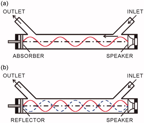
The acoustic treatment in a standing-wave agglomerator can achieve higher particle removal efficiency than a travelling field under the same power consumption due to the superposition of the incident wave and reflected wave. In a travelling wave field without attenuation, the acoustic velocity at any point in a gas medium possesses identical amplitudes. On the other hand, for a standing wave field, the acoustic velocity amplitude is varied along the propagation direction as shown in Figure 4. Consequently, given the lack of spatial considerations, the conventional temporal aerosol dynamic models are incapable of simulating the acoustic agglomeration in a standing wave field.

Figure 4. Illustration of the travelling wave and standing wave in an acoustic agglomerator.

To resolve for the effects of standing waves on acoustic agglomeration, the acoustic velocity and spatially varying kernels have to be first defined. The acoustic velocity of the air at position x and time t of a one-dimensional standing wave field can be described as (21) where U_g0 is the acoustic velocity amplitude, k is the wave number, and f is the sound frequency.

The acoustic kernels for orthorkinetic and hydrodynamic interactions in a travelling wave field can be extended to a standing wave field by substituting the local acoustic velocity amplitude into Equations (10)(10) and (13)(13) (22) (23)

Yan et al. (2016) experimentally investigated the effect of humidity on the acoustic agglomeration in a standing wave field and found that in a low supersaturation degree S = 0.3 (S is defined as the ratio of the partial pressure of water vapor to its equilibrium vapor pressure), the influence of water droplets on particle agglomeration was negligible. Herein, the experimental data for the supersaturation degree S = 0.3 are used as a typical case to demonstrate the application of the spatial sectional model in the standing-wave agglomeration. The aerosol is re-dispersed coal ash with the aerodynamic diameter of the particles between 0.023 µm and 9.314 µm. The sound frequency of the standing wave field is 1.8 kHz and the SPL is 150 dB at every half wavelength from the acoustic source. The distance between the inlet and sampling point in the acoustic chamber is equal to 5 wavelengths (944 mm), and the residence time is 2.5 s. The operation pressure and temperature are 1 atm and 293 K, respectively.

The particle size distribution by simulation (square) at the outlet of the acoustic chamber is presented in Figure 5 with comparison to the experimental measurement (triangle) for the same initial distribution (diamond). It can be observed from the area under the particle size distribution curve that the number concentration of the particles in submicron range decreases strikingly for both numerical simulation and experiments, indicating the occurrence of the particle agglomeration. The predicted particle size distribution is basically agreeable with the experimental data, and the actual discrepancy between simulations and experiments is expected to be smaller than what it is currently since the agglomeration caused by humidity condensation is not taken into account in the simulations. 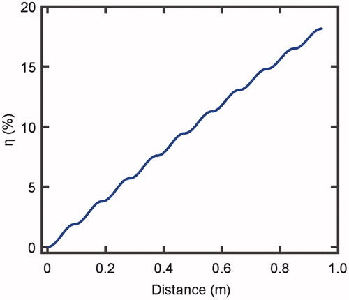For quantitative analysis, the efficiency for acoustic agglomeration can be defined by (24) where N and N₀ are the total number concentration of the particles at some position and at the inlet, respectively. The agglomeration efficiency is plotted with the agglomerator distance from the sound source in Figure 6. As observed, agglomeration efficiency of the particles increases from 0 at the inlet to 18.2% at the outlet of the chamber, indicating a clear spatial effect on the agglomeration process. Besides, it’s also worth noting that the agglomeration efficiency is not increased linearly but in an intermittent way, which is ascribed to the spatial alternation of the acoustic kernel from the velocity node to antinode. The spatial variation of the acoustic agglomeration efficiency shown in Figure 6 demonstrates that it is more reasonable to conduct the simulation in a standing wave field by solving the spatial sectional model rather than the conventional temporal model.

Figure 5. Simulation results (square) compared with experimental measurements (triangle) of the particle size distribution in a standing wave field. The initial distribution (diamond) of the aerosol at the chamber inlet is also included.

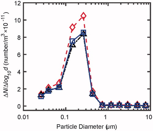
Figure 6. The predicted efficiency of acoustic agglomeration as a function of spatial position along the agglomerator. The agglomeration efficiency is increased in an intermittent way, which is ascribed to the spatial alternation of the acoustic kernel from the velocity node to antinode.

3.3. Sound attenuation by aerosol particles in a travelling field

In the previous numerical studies, the SPL is regarded as equal all over the whole agglomerator. However, in reality, the SPL may drop considerably due to particulate–medium interaction. Thus, the influence of sound attenuation in acoustic agglomeration is investigated in this section. To comprehend the effects of sound attenuation, the agglomeration kernel in an acoustic field, which is attenuated by particulate matters, is derived at first and then the spatial sectional model is applied to simulate the acoustic agglomeration process.

The acoustic attenuation in particulate medium is mainly caused by two dissipation mechanisms: the particle relaxation by viscosity and the heat transfer from the gas medium to particles. The thermal relaxation time for a particle of density ρ_p and diameter d are calculated by (25) where Pr is the Prandtl number, μ is the dynamic viscosity of the gas, C_p and C_pg are the specific heat of the particle and gas, respectively, and the dynamic relaxation time is defined by Equation (12)(12) .

The sectional expression of the attenuation coefficient σ_l in the l-th section can be approximated by the energy-dissipation method proposed by Temkin (1981), (26) where N_l and d_m are the number concentration and average diameter of the particle in the l-th section, and ρ_g and κ are the density and specific heat ratio of the air, respectively.

The acoustic velocity amplitude is related to the attenuation coefficient by (27) where U_g0 is the acoustic velocity amplitude at the sound source.

Substituting Equation (27)(27) into Equations (10)(10) and (13)(13) , we can immediately derive the acoustic kernels for the orthokinetic interaction and hydrodynamic interaction with attenuation effects (28) (29)

It can be seen that the acoustic kernels with sound attenuation are varied with the space position and accordingly the acoustic agglomeration becomes nonhomogeneous, and the spatial sectional model should be applied rather than the conventional temporal model.

In most literatures, information about the acoustic field and aerosol properties is usually incomplete, and the sound pressure given by the authors is the average value at several sampling points. To the best of the authors’ knowledge, there is no experimental data to form a basis for comparison on the effects of sound attenuation on acoustic agglomeration at this stage. Hence, to appreciate the effects of sound attenuation, a characteristic acoustic chamber is selected as the agglomerator with the length of 2.5 m and the residence time of 5 s. The aerosol of glycol, which is from the experiment by Caperan et al. (1995) under a closed-chamber condition, is employed as the representative aerosol at the inlet. The size distribution is log-normal with a geometric mean diameter of 0.8 µm and standard deviation of 1.3. The number concentration N₀ at the inlet is 3.8 10⁶ cm⁻³ and the particle density is 1115 kg/m³. Here, apart from the two frequencies adopted by Caperan et al. (1995), 10 kHz and 21 kHz, two more frequencies at 2 kHz and 5 kHz are also simulated. This allows us to understand the effects of a wide range of frequencies on the sound attenuation. For all cases, the SPL at the sound source is equal to 150 dB.

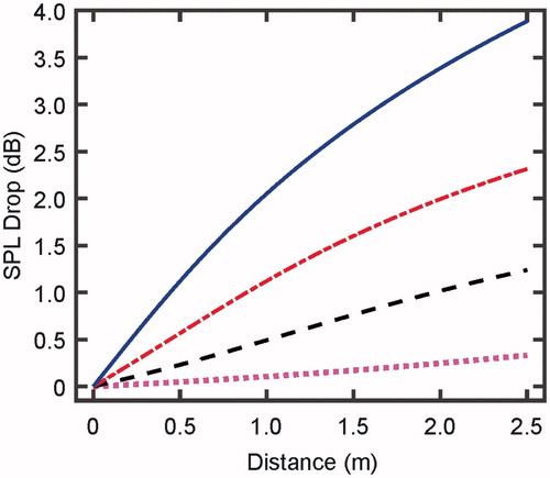
The attenuation coefficients at four frequencies (2 kHz for dotted line, 5 kHz for dashed line, 10 kHz for dot-dashed line, and 21 kHz for solid line) are illustrated with respect to the distance from the aerosol inlet in Figure 7. It can be seen that the attenuation coefficient at each frequency is not constant but varies in a complex way. For the frequency of 10 kHz and 21 kHz, it increases slightly at first and then decreases rapidly with the wave propagation, and the value at the outlet of the chamber could be a half of that at the inlet. The attenuation coefficient at low frequencies (2 kHz and 5 kHz) is much smaller than at high frequencies on the whole and also undergoes smoother variation along the propagation direction. The attenuation of the acoustic field results from the sound-particle interaction, including the kinetic energy dissipation and heat transfer from sound to the particle. Generally, the attenuation effect tends to be enhanced with increasing number concentration and particle size. Thus, the acoustic agglomeration has double-sided impact on the attenuation coefficient. With the progress of acoustic agglomeration, the attenuation coefficient increases with the enlarged particle size and weakens with the reduction of the number concentration. On the other hand, the growth or decrease of the attenuation coefficient of the sound field can weaken or enhance the acoustic agglomeration, which again affects the number concentration and particle size. Consequently, the attenuation is interactive with the acoustic agglomeration, which leads to the complex variation of the attenuation coefficient as shown in Figure 7. As long as the attenuation coefficient is not equal to zero, the sound pressure drops down continuously along the propagation direction as shown in Figure 8. The total SPL drop at four frequencies is approximately 3.90 dB for 21 kHz, 2.31 dB for 10 kHz, 1.25 dB for 5 kHz, and 0.33 dB for 2 kHz, respectively. Apparently, the sound attenuation is augmented with increasing frequencies. For this typical aerosol, the sound attenuation at 10 kHz and 21 kHz leads to the reduction of acoustic velocity for about a half at the outlet of the agglomerator, which is too significant to overlook in the simulation of acoustic agglomeration.

Figure 7. The variation of the attenuation coefficients with respect to the distance from the inlet in the agglomerator at four frequencies: 2 kHz (dotted), 5 kHz (dashed), 10 kHz (dot-dashed), and 21 kHz (solid).

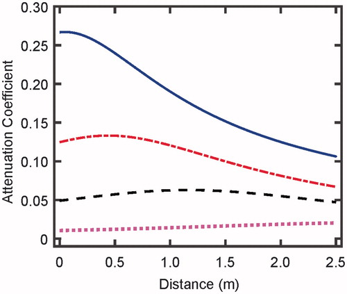
Figure 8. Dependence of the SPL drop on the distance from the inlet in the agglomerator at four frequencies: 2 kHz (dotted), 5 kHz (dashed), 10 kHz (dot-dashed), and 21 kHz (solid).

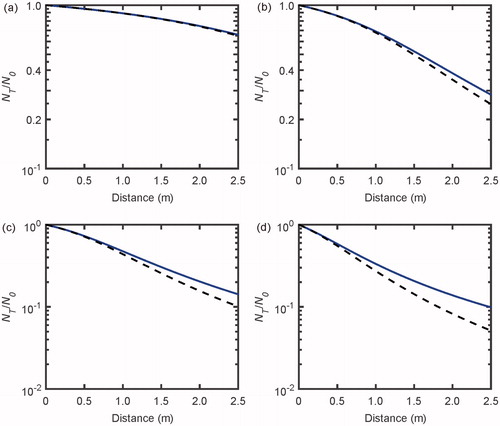
The normalized number concentration N_T for acoustic agglomeration with (solid line) and without (dashed line) attenuation effect is plotted as a function of the space position in Figure 9 for four frequencies: (a) 2 kHz, (b) 5 kHz, (c) 10 kHz, and (d) 21 kHz. As observed, particle number concentration drops down evidently with the acoustic direction for all cases, indicating that an enormous number of particles form into agglomerates. The number concentrations at the outlet for the acoustic field without attenuation at 2 kHz, 5 kHz, 10 kHz, and 21 kHz are 0.65, 0.25, 0.1, and 0.05, respectively. Obviously, for this typical aerosol considered here, the agglomeration effect is enhanced with increasing frequencies, which is related to the optimum frequency and not the focus of the current study. The impact of sound attenuation on the acoustic agglomeration differs with the varied frequencies, which can be attributed to the different attenuation coefficients. At high frequencies, the noticeable discrepancy between two predictions continues from the inlet to the outlet. For example, at 21 kHz, the outlet number concentration with attenuation is reduced to 0.1N₀, which is approximately twice of that without attenuation, 0.05N₀. However, the attenuation plays an insignificant role in the acoustic agglomeration at low frequencies or even negligible at 2 kHz. Therefore, we can speculate that at high frequencies, omission of the sound attenuation effect will cause overestimate of the agglomeration rates in the simulation of acoustic agglomeration. Ezekoye and Wibowo (1999) compared the simulation results with the experimental data at 10 kHz reported by Caperan et al. (1995), and found that the simulation results were strikingly larger than the experimental results. Based on the present findings, we can conclude that the omission of sound attenuation in their simulation could be responsible for the overprediction of the acoustic agglomeration rate in addition to the limitation of the existing acoustic kernels.

Figure 9. The dependence of the normalized number concentration N_T for acoustic agglomeration with (solid line) and without (dashed line) attenuation effect on the space position for four frequencies: (a) 2 kHz, (b) 5 kHz, (c) 10 kHz, and (d) 21 kHz.

4. Conclusions

In summary, a one-dimensional spatial sectional model of the aerosol dynamic equation that can overcome existing limitations of conventional temporal model is established to investigate the nonhomogeneous acoustic agglomeration in the present study. The sectional aerosol dynamic equation incorporates the convective transport of aerosols, and the acoustic kernels are included as sectional source terms. Two practical scenarios of nonhomogeneous acoustic agglomeration are investigated by the spatial sectional model. The following conclusions can be drawn from the current findings:

1. The present model overcomes the inherent drawbacks of the widely adopted numerical scheme developed by Song. It integrates the agglomeration kernel over the whole section and calculates all the general quantities of an aerosol directly. The comparison between the predictions of the present model and Song’s algorithm shows that the present sectional model can achieve comparable or better computation accuracy using a much smaller number of sections.

2. The acoustic kernels in a standing wave field are dependent on the space position due to the alternation of the acoustic velocity between nodes and antinodes, which makes the conventional temporal model incapable to simulate the standing-condition agglomeration. The particle size distribution simulated by the present spatial sectional model is basically agreeable with the experimental data by Yan et al. Based on this, the agglomeration efficiency is found to increase in an intermittent way along the agglomerator, which confirms the rationality to simulate a standing-wave agglomeration through the spatial sectional model rather than the conventional temporal model.

3. Acoustic attenuation caused by the sound-particle interaction in the particulate medium is simulated by the spatial sectional model. It shows that with increasing frequency, the sound attenuation and its impact on acoustic agglomeration is enhanced. At high frequencies, the sound attenuation plays a significant role in the acoustic agglomeration process and omission of this factor can result in overestimations of the agglomeration rates in the simulation of acoustic agglomeration.

Nomenclature
c	=	sound speed
Cp	=	specific heat
d	=	particle diameter
D	=	diffusion coefficient
f	=	sound frequency
g12	=	hydrodynamic interaction function
H	=	entrainment factor
k	=	wave number
kB	=	Boltzmann constant
M	=	aerosol mass concentration
n	=	particle size distribution function
N	=	aerosol number concentration
P	=	gas pressure
Pe	=	Peclet number
Pr	=	Prandtl number
q	=	general property of aerosol
Q	=	general integral quantity of aerosol
R	=	gas constant
Re	=	Reynolds number
S	=	source term
t	=	time
T	=	temperature
	=	particle velocity by convection
	=	particle velocity by external force
ug	=	acoustic velocity of gas
Ug	=	acoustic velocity amplitude of gas
Ug0	=	Ug at sound source
up	=	particle velocity
Ux	=	mean flow velocity in x direction
v	=	particle volume
	=	particle volume
V	=	aerosol volume concentration
	=	space vector
α	=	parameter
β	=	agglomeration kernel
γ	=	parameter
η12	=	real part of entrainment factor H12
κ	=	specific heat ratio
µ	=	dynamic viscosity of gas medium
ρ	=	density of gas medium
σ	=	attenuation coefficient
τd	=	dynamic relaxation time
τt	=	thermal relaxation time
ω	=	angular frequency

Additional information

Funding

This study is supported by the Republic of Singapore's Ministry of Education through grant no. RG190/14 and MOE2016-T2-1-063.

References

- Bush, P. V., and Snyder, T. R. (1992). Implications of Particulate Properties on Electrostatic Precipitator and Fabric Filter Performance. Powder Technol., 72:207–213.
- Caperan, Ph., Somers, J., Richter, K., and Fourcaudot, S. (1995). Acoustic Agglomeration of a Glycol Fog Aerosol: Influence of Particle Concentration and Intensity of the Sound Field at Two Frequencies. J. Aerosol Sci., 26:595–612.
- Ezekoye, O. A., and Wibowo, Y. W. (1999). Simulation of Acoustic Agglomeration Processes Using a Sectional Algorithm. J. Aerosol Sci., 30:1117–1138.
- Fan, F., Zhang, M., Peng, Z., Chen, J., Su, M., Moghtaderi, B., and Doroodchi, E. (2017). Direct Simulation Monte Carlo Method for Acoustic Agglomeration under Standing Wave Condition. Aerosol Air Qual. Res., 17:1073–1083.
- Friedlander, S. K. (2000). Smoke, Dust, and Haze: Fundamentals of Aerosol Dynamics. Oxford University Press, New York, p. 309.
- Gallego-Juarez, J. A., Riera, E., Rodriguez, G., Hoffmann, T. L., Galvez, J. C., Rodriguez, J. J., Gomez, F. J., Bahillo, A., and Martin, M. (1999). Application of Acoustic Agglomeration to Reduce Fine Particle Emissions from Coal Combustion Plants. Environ. Sci. Technol., 33(21): 3843–3849.
- Gelbard, F., and Seinfeld, J. H. (1980). Simulation of Multicomponent Aerosol Dynamics. J. Colloid Interface Sci., 78:485–501.
- Hoffmann, T. L. (1997). An Extended Kernel for Acoustic Agglomeration Simulation based on the Acoustic Wake Effect. J. Aerosol Sci., 28:919–936.
- Kim, J. C., and Lee, K. W. (1990). Experimental Study of Particle Collection by Small Cyclones. Aerosol Sci. Technol., 12:1003–1015.
- Lee, K. W., and Liu, B. Y. H. (1981). Experimental Study of Aerosol Filtration by Fibrous Filters. Aerosol Sci. Technol., 1:35–46.
- Lee, P. S., Cheng, M. T., and Shaw, D. T. (1981). The Influence of Hydrodynamic Turbulence on Acoustic Turbulent Agglomeration. Aerosol Sci. Technol., 1:47–58.
- Ma, D., Zheng Q., Lin W., and Guo M. (2017). Improvements to Dust Filtration through Acoustic Agglomeration and Atomization. Aerosol Sci. Technol., 51:824–832.
- Malherbe, C., Boulaud, D., Boutier, A., and Lefevre, J. (1988). Turbulence Induced by an Acoustic Field Application to Acoustic Agglomeration. Aerosol Sci. Technol., 9:93–103.
- Mednikov, E. P. (1965). Acoustic Coagulation and Precipitation of Aerosols. Consultants Bureau, New York.
- Ng, B. F., Xiong, J. W., and Wan, M. P. (2017). Application of Acoustic Agglomeration to Enhance Air Filtration Efficiency in Air-Conditioning and Mechanical Ventilation (ACMV) Systems. PLOS ONE, 12:e0178851.
- Pope, C. A., III. (2000). Review: Epidemiological Basis for Particulate Air Pollution Health Standards. Aerosol Sci. Technol., 32:4–14.
- Riera, E., Gonzalez-Gomez, I., Rodriguez, G., and Gallego-Juarez, J. A. (2015). Power Ultrasonics: Applications of High-Intensity Ultrasound. Woodhead Publishing, Cambridge, p. 1043.
- Riley, W. J., Mckone, T. E., Lai, A. C. K., Nazaroff, W. W. (2002). Indoor Particulate Matter of Outdoor Origin: Importance of Size-Dependent Removal Mechanisms. Environ. Sci. Technol., 36:200–207.
- Sarabia, E. R. F., Elvira-Segura, L., Gonzalez-Gomez, I., Rodriguez-Maroto, J. J., Munoz-Bueno, R., and Dorronsoro-Areal, J. L. (2003). Investigation of the Influence of Humidity on the Ultrasonic Agglomeration of Submicron Particles in Diesel Exhausts. Ultrasonics, 41:277–281.
- Sarabia E. R. F., and Gallego-Juarez, J. A. (1986). Ultrasonic Agglomeration of Micron Aerosols under Standing Wave Conditions. J. Sound Vib., 110:413–427.
- Shaw, D. T., and Tu, K. W. (1979). Acoustic Particle Agglomeration due to Hydrodynamic Interaction between Monodisperse Aerosols. J. Aerosol Sci., 10:317–328.
- Sheng, C., and Shen, X. (2006). Modelling of Acoustic Agglomeration Processes Using the Direct Simulation Monte Carlo Method. J. Aerosol Sci., 37:16–36.
- Sheng, C., and Shen, X. (2007). Simulation of Acoustic Agglomeration Processes of Poly-Disperse Solid Particles. Aerosol Sci. Technol., 41:1–13.
- Sheriff, N., and O’Kane, D. J. (1971). Eddy Diffusivity of Mass Measurements for Air in Circular Duct. Int. J. Heat Mass Transfer, 14:697–707.
- Sitarski, M., and Seinfeld, J. H. (1977). Brownian Coagulation in the Transition Regime. J. Colloid Interface Sci., 61:261–271.
- Song, L. (1990). Modelling of Acoustic Agglomeration of Fine Aerosol Particles. PhD thesis, The Pennsylvania State University, USA.
- Song, L., Koopmann, G. H., and Hoffmann, T. L. (1994). An Improved Theoretical Model for Acoustic Agglomeration. J. Vib. Acoust., 116:208–214.
- Temkin, S. (1981). Elements of Acoustics. John Wiley & Sons, New York, p. 459.
- Tiwary, R., and Reethof, G. (1987). Numerical Simulation of Acoustic Agglomeration and Experimental Verification. J. Vib. Acoust. Stress and Reliab., 109:185–191.
- Yan, J., Chen, L., and Yang, L. (2016). Combined Effect of Acoustic Agglomeration and Vapor Condensation on Fine Particles Removal. Chem. Eng. J., 290:319–327.
- Yuen, W. T., Fu, S. C., and Chao, C. Y. H. (2016). The Correlation between Acoustic Streaming Patterns and Aerosol Removal Efficiencies in an Acoustic Aerosol Removal System. Aerosol Sci. Technol., 50:52–62.
- Yuen, W. T., Fu, S. C., Kwan, J. K. C., and Chao, C. Y. H. (2014). The Use of Nonlinear Acoustics as an Energy-Efficient Technique for Aerosol Removal. Aerosol Sci. Technol., 48:907–915.
- Yuen, W. T., Fu, S. C., and Chao, C. Y. H. (2017). The Effect of Aerosol Size Distribution and Concentration on the Removal Efficiency of an Acoustic Aerosol Removal System. J. Aerosol Sci., 104:79–89.
- Zhao, H., and Zheng, C. (2013). A Population Balance-Monte Carlo Method for Particle Coagulation in Spatially Inhomogeneous Systems. Comput. Fluids, 71:196–207.