Growth rate and oscillation frequency of electrified jet and droplet: Effects of charge and electric field

Abstract

Electrified jets are applied industrially in agriculture, automobiles, targeted drug delivery systems, spacecraft propulsion units, liquid metal sprayers, ion sources, emulsifiers, dust scavenging systems, and ink-jet printers. Electrified columnar jets experience instability caused by electrohydrodynamic interactions of the charged liquid surfaces with electric fields. Electrostatic and surface tension forces competing along the liquid surface create surface pressure differences. The temporal rise and fall of the surface pressure induce oscillations of jets and droplet. A linear theory was derived to yield a dispersion equation determining the most dominant wavelength of oscillation for a given charge level and electric field; this enabled the estimation of the diameter of an atomized droplet. In addition, the frequency of oscillation was derived for a cylindrical jet and spherical droplet. Parametric studies were performed for various charging levels and electric field strengths.

© 2018 American Association for Aerosol Research

EDITOR:

• Warren Finlay

1. Introduction

Electrostatic atomization techniques are used to produce extremely fine electrified jets for many applications, including agricultural and automotive sprays, targeted drug delivery systems, spacecraft propulsion units, liquid metal sprayers, ion sources, emulsifiers, dust scavenging systems, and ink-jet printers. To create such jets, liquid emanating from a needle or orifice is charged with a high voltage while the spray target or substrate is electrically grounded with the opposite charge. This forms an electric field between the orifice and the target substrate.

For a positively charged orifice, negatively charged ions in the liquid are attracted to the charged needle within the liquid, while positively charged ions migrate toward the liquid surface at the orifice exit. The negatively charged substrate attracts the positively charged ions at the liquid surface, electrically pulling them toward the substrate against the resistance provided by surface tension. This competition between electrostatic forces and surface tension creates a Taylor (1964, 1969) cone. During liquid attraction, a thin thread of charged liquid is formed at the tip of the Taylor cone. This thin liquid thread is inherently unstable and eventually becomes atomized into a fine spray of droplets. The instability of such electrified jets is of scientific interest regarding the estimation of the size of atomized droplets.

The dynamics of the charged liquid jet is greatly influenced by the charging level (V₀) and the strength of the electric field, which is determined by the distance between the charged orifice and the ground location a/b, where a and b are the jet radius and distance to ground, respectively. Interactions between the surface charges on the liquid surface and the electric field imposed by the charges and the ground location induce changes in the electrically perturbed pressure, which compete with the surface tension pressure of the liquid. Both the statics and dynamics of electrified jets and droplets have received significant research attention.

Basset (1894) first derived a dispersion equation providing a growth rate relation for electrified jets. However, Basset’s equation included a sign error in front of the modified Bessel function of the second kind K_m(k). Schneider et al. (1967) made the same mistake, as noted by Neukermans (1973), who claimed that Schneider et al. neglected to expand various terms up to the second order. All electrostatic energy terms should be of the second order because of the nonlinear sinusoidal wave assumption. Neukermans’ dispersion equation uses the correct sign in front of K_m(k); however, Neukermans incorrectly described his equation as consistent with that of Basset, which is false because of Basset’s sign error. This suggests that Neukermans was unaware of Basset’s mistake.

Taylor (1969) noted Basset’s sign error and provided a correct dispersion equation while using the Bessel function expression from Watson (1922). Taylor’s dispersion equation is thus equivalent to that of Neukermans. Melcher (1963) had already provided a correct expression of the dispersion equation for an electrified jet; however, this dispersion equation was difficult to follow, and his expression included the Bessel and Hankel functions of the first and second kinds, their derivatives, and a complex argument. Therefore, Melcher’s expression appeared dramatically different from those derived by Taylor (1969) and Neukermans (1973). Although Taylor (1969) and Neukermans (1973) provided correct dispersion equations, their expressions were limited to the mode number of m = 0 only. The general expression for all modes must be obtained, as the electrified jet undergoes completely different instability processes for different oscillatory modes. This general expression should provide solutions for all mode values, thus enabling parametric studies. Artana et al. (1998) and Li et al. (2005) also produced a general dispersion equation that included the mode number. However, the dispersion equation appeared to be quite different from that of Taylor (1969) and Neukermans (1973) and thus a direction comparison was not possible. Computational studies regarding detailed instability phenomena were conducted by several groups; Setiawan and Heister (1997), Lopez-Herrera et al. (1999), and Collins et al. (2007). These groups computationally addressed both linear and nonlinear distortion of an electrified jet. Herein, we, for the first time worldwide, provide analytic solutions for the dispersion equation of an electrified jet for various values of the charging level (V₀ or a dimensionless term of Γ_e), electric field (a/b), and instability mode (m).

For a two-dimensional (2D) electrified cylindrical jet or three-dimensional (3D) spherical droplet, the charged surface undergoes oscillation because of the competing actions of the surface tension and electrostatic force. The electrostatic force tends to disrupt or push away from the surface, while the surface tension tends to pull or minimize surface area. The rise and fall of the charged surface can be modeled by a sinusoidal wave as a function of the mode (m) and time (t) using a linear expression, in which the growth rate (ω) appears as an exponent within a temporal term. For example, the wave surface η grows proportionally with ∼ e^ωt. In detail, ω is a complex number ω = ω_r+ω_i, where the real part (ω_r) defines the growth rate and the imaginary part (ω_i) defines the frequency of oscillation. While the growth rate or dispersion equation is expressed in terms of ω², the frequency of oscillation must be explicitly expressed using ω_i alone.

Rayleigh (1882) was the first to derive the frequency of oscillation ω_i of an electrified cylindrical jet and spherical droplet; his work is widely cited by many authors. However, many students and researchers are frustrated by the archaic mathematical notation and intermediate omission in Rayleigh’s model. Hendricks and Schneider (1963) revisited the Rayleigh expression for the frequency of oscillation for spherical droplets; however, detailed derivations for 2D cylindrical jets have not yet been provided in the literature. In addition, the frequency of oscillation derived by Rayleigh (1882) neglects the effects of the ground location, and thus the effect of electric fields cannot be accurately quantified using Rayleigh’s model. We address this issue of electric fields in this report by including the effect of the ground location in our final expression.

2. Growth rate or dispersion equation of an electrified jet

The existence of minute system disturbances can induce instability on the jet surface. Rayleigh showed that, among all disturbance components, those with wavelengths exceeding the circumference of the unperturbed jet cause the breakup of the jet. He also established that components having the dimensionless wavenumber of 0.696 experience the maximum growth rate, thus dominating the breakup. Higher growth rates correspond to faster growths of disturbance, which in turn indicate faster breakup and shorter breakup lengths. Hence, the wave with the maximum growth rate has the shortest breakup length.

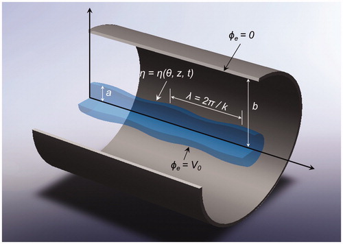
In accordance with a standard Fourier (normal mode) analysis, we presume an infinitesimal disturbance in the surface shape of the form: (1) which represents an infinite wave train traveling in the axial (z) direction with the axial wavenumber growing at the rate ω_r in the time . Figure 1 shows a 3D mode illustration. The assumed form for η does not permit the modeling of helical instabilities. Rayleigh (1878) showed that axisymmetric modes grew at the fastest rate for purely capillary instabilities. For most conditions of interest in electrostatic spraying applications, this conclusion is valid; however, helical modes can grow preferentially at very high charging levels (Melcher 1963). Those with an interest in these modes are referred to Melcher’s (1963) work.

Figure 1. Schematic of a 3D Mode.

In general, the axial () and radial (v) velocities are defined as: (2) (3) where U and V are the mean flow velocities and are the perturbation flow velocities. Because the coordinate system is assumed to move axially with the jet, the axial velocity is the perturbation velocity (). The radial velocity is also the perturbation velocity () because the mean radial velocity is zero (). Therefore, we may define the electrostatic and velocity potentials and , which obey the relationships: (4) (5) where and are the perturbations of the electrostatic and velocity potentials, respectively. Solving for , we obtain: (6) where is the zeroth-order solution for a charged cylinder. Let . Then, applying the boundary conditions and at and (see Figure 1), respectively, we obtain: (7) which satisfies Laplace’s equation. In order to satisfy , a separable solution is assumed: (8)

For cylindrical coordinates, Laplace’s equation is (9)

Differentiation of Equation (8)(8) with respect to,, and gives (10)

This Bessel equation has the solution (11) where is a modified Bessel function of the first kind and is a modified Bessel function of the second kind. Therefore, can be written as: (12)

Applying the boundary conditions and 0 at and, respectively, and using the following linear approximation: (13) (14) (15)

The values and are evaluated as (16) (17)

Rewriting Equation (12)(12) with and yields (18) where (19)

The solution for also involves Bessel functions: (20)

The modified Bessel function of the second kind, , approaches infinity as approaches zero. To have a finite value at which equals zero, must be zero. Assuming irrotational flow, can be evaluated by applying the kinematic conditions as follows: (21) (22)

Taking the substantial derivative at, (23)

Because is only a function of, and (24) where (25) (26)

By neglecting higher-order terms, the second-order kinematic condition at becomes: (27)

Appling this kinematic condition to Equations (1)(1) and (20)(20) gives (28) and (29)

To determine our dispersion equation , we must include the Bernoulli equation at the surface. The Bernoulli equation states that changes in with time are driven by the perturbation of the electrostatic pressure on the surface. By writing the Bernoulli equation from the undisturbed upstream region to the disturbed downstream region, the applicable form is (30)

Neglecting , , Ω (the body force), and , and linearizing , we obtain the following expression: (31) where is the capillary pressure on the undisturbed surface and is the capillary pressure on the disturbed surface due to electrostatics. The sum of the electrostatic and capillary pressures is compensated by the surface tension: (32) (33) where (34) (35) (36) in which is the surface tension, is the electrostatic density charge (see Wangsness 1986), is the curvature of the surface, and are the undisturbed and disturbed electrostatic pressures, respectively. Differentiating Equation (7)(7) with respect to and evaluating at gives , which can be used to evaluate from Equation (34)(34) : (37)

Using Equations (32)–(37) yields another expression for Equation (31)(31) , which is (38)

The challenge here is to express at. Previously, we found that for an undisturbed surface. While this is not fully accurate for a disturbed surface, we still approximate, (39)

By differentiating Equation (12)(12) with respect to r, we obtain, (40)

Using, (41) (42)

Equation (40)(40) can be rewritten as, (43)

We now have all the expressions necessary to rewrite Equation (38)(38) . By substituting Equations (29)(29) , (36)(36) , and (43)(43) into Equation (38)(38) , we obtain the dispersion equation. (44)

In order to complete the analysis, we expand and . Differentiating Equation (19)(19) at yields: (45)

approaches zero when kb ≫ 1, by the nature of the modified Bessel function of the second kind. From Bessel differentiation, we know that: (46) (47)

Substituting Equation (47)(47) into Equation (45)(45) yields: (48)

Substituting Equations (46)(46) and (48)(48) into Equation (44)(44) obtains: (49)

It is worthwhile to note that we only considered the relatively long waves because of the fundamental assumption of ka < 1 or λ/a > 2π. For the short-wave limit of ka → ∞, this would result in the Kelvin–Helmholtz case, which focuses on relative very small wavelengths. The effect of electrical charges on a liquid jet must be restricted to a cylindrical case, which in turn assumes a relatively finite length-scale of the jet dimension. This restriction inevitably introduces visible or relatively large wavelengths of ka < 1 or λ/a > 2π. In other words, if ka → ∞ or λ/a ≪ 2π (which is the Kelvin–Helmholtz case), the wavelength scale would be too small to be affected by any electrical charges.

We now denote each dimensional term using and then apply the following three characteristic parameters to nondimensionalize Equation (49)(49) : (50) (51) (52)

The complete nondimensionalized dispersion equation is therefore expressed as: (53)

This agrees with the work of Taylor (1969), Melcher (1963), and Neukermans (1973), in which the dispersion equations were derived by considering the forces on a surface element; see Table 1. Here, is the nondimensional axial wavenumber, m is the circumferential wavenumber, and ω is the nondimensional growth rate, which provides the speed of column distortion. The nondimensional column radius is a, while b is the ground location; thus, a is unity. The nondimensional parameter governs the physics of the flow-field. is the permittivity of free space. σ′ and V₀′ represent the surface tension and applied voltage, respectively. Γ_e is the ratio of electrostatic to capillary pressures generated at the surface of the column. In a 2D analysis, the electrostatic potential grows logarithmically (Equation (18)(18) ); thus, we place the ground location at some finite distance from the surface.

Table 1. Summary of the dispersion equations for an electrified jet of various authors.

References	Dimensional equation
Melcher (1963)
Taylor (1969)
Neukermans (1973)
Present

Taylor (1969) and Neukermans (1973) assumed m = 0. All of these equations are dimensional.

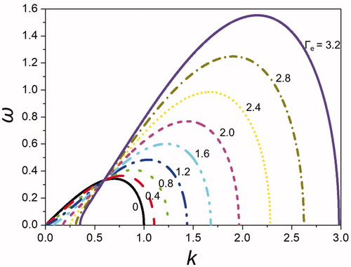
Figure 2 shows the solution of the growth rate or dispersion Equation (53)(53) for various charging levels Γ_e of 0–3.2 for the mode number m = 0. At the charging level of zero, the maximum growth rate corresponds to the nondimensional wavenumber of k = 0.69; this value is exactly equal to Rayleigh’s (1878) result, which predicted the most dominant wavelength of λ = 2π/k = 9 for an uncharged jet. As the charge level is increased, the wavenumber k increases, which means the wavelength λ decreases. Increased electrostatic charges induce the appearance of shorter wavelengths while the electrostatic force competes against the surface tension force.

Figure 2. Effect of the charging level Γ_e on the growth rate ω at m = 0 and b/a = 10.

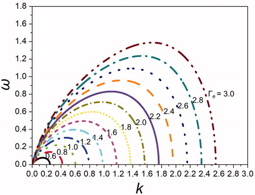
Figure 3 shows the solution of the growth rate or dispersion Equation (53)(53) for various charging levels Γ_e of 0.6–3 for the increased mode number m = 1. As observed in Figure 2, here, the wavenumber k_opt corresponding to the maximum growth rate also increases for increased Γ_e; again, as the electrostatic charge increases, the wavenumber k increases and the corresponding wavelength λ decreases. It should be noted that, for the increased mode number of m = 1, greater electrostatic strength is required in order to destabilize the jet. For m = 1, the minimum electrostatic charge required to induce jet instability is approximately Γ_e = 0.6.

Figure 3. The effect of the charging level Γ_e on the growth rate ω at m = 1 and b/a = 10.

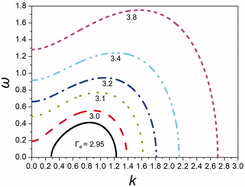
Figure 4 shows the solution of the growth rate or dispersion Equation (53)(53) for various charging levels Γ_e of 2.95–3.8 for the mode number m = 2. Herein, the growth rate (ω) is greater than zero even when the wavenumber k is zero; this indicates that the jet is intrinsically unstable even for an infinitely long wavelength (or the wavenumber k = 0). It should also be noted that the minimum electrostatic strength required for jet instability is approximately Γ_e ∼ 2.95. Once jet instability is initiated (Γ_e ≥ 2.95), the jet is unconditionally unstable for all wavenumbers when m ≥ 2.

Figure 4. Effect of the charging level Γ_e on the growth rate ω at m = 2 and b/a = 10.

In Figures 2–4, the growth rates at various charge levels and mode numbers (m = 0, 1, and 2) are plotted for the given jet-to-ground distance of b/a = 10. When the distance is reduced to b/a = 2.71, the electrostatic strength (E) is magnified because the electrostatic field is inversely proportional to the distance (r); E ∝ 1/r. The growth rates at this reduced distance are plotted in Figure 5.

Figure 5. Effect of the charging level Γ_e on the growth rate ω for various modes of (a) m = 0, (b) m = 1, (c) m = 2, (d) m = 3, (e) m = 4, and (f) m = 5 at b/a = 2.71.

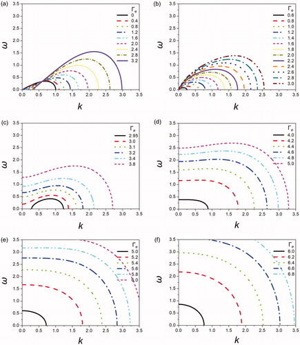
Figure 5 compares the growth rates acquired at various mode numbers (m = 0, 1, 2, 3, 4, and 5) and electrostatic charge levels. As shown previously, the minimum electrostatic charge level (Γ_e) is increased as the mode number increases; this means that greater Γ_e values are needed to induce instability in higher-mode jets. The jet surface area is increased as the mode number increases. Therefore, greater numbers of surface charges are required to render the jet unstable. This trend is clearly shown when comparing the growth rates of m = 3 and 4, shown in Figures 5d and e, respectively. For the constant Γ_e = 5, the growth rate nears ω ∼ 2.5 for m = 3 while the growth rate approaches ω ∼ 0.6 for m = 4. Clearly, the higher mode is less susceptible to destabilization while experiencing a smaller growth rate. Overall, this means that a greater electrostatic charge is required for the destabilization of higher-mode cases. As shown before in cases of b/a = 10, the growth rates are greater than zero even when k = 0 for the mode number m ≥ 2. This result indicates that the jets are unconditionally unstable even for infinitely long waves at higher modes of m ≥ 2.

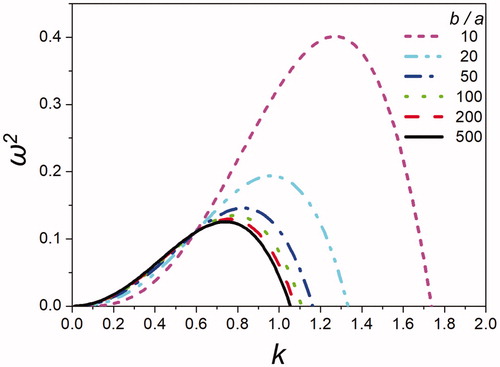
Figure 6 shows the effect of the ground location b/a, which determines the strength of the electric field, on the growth rate. As the ground location approaches the jet, that is, as b/a is decreased, the electrostatic force increases, which in turn increases the wavenumber k and decreases the wavelength λ. For ground locations sufficiently far from the electrified jet, no electric field is imposed, and the electrified jet is equivalent to a nonelectrified jet. This pattern manifests for the case b/a = 500 in Figure 6, as the maximum growth rate is reached for the corresponding wavenumber k_opt = 0.69, which is Rayleigh’s result for nonelectrified jets.

Figure 6. Effect of the ground location b/a (or electric field) on the growth rate squared (ω²) at Γ_e = 9.

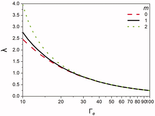
Figure 7 quantitatively compares the growth rate variation with changes in mode. Under the same charging level and electric field strength, the growth rate maximum is shifted toward the left, indicating a decrease in wavenumber and increase in wavelength as the mode number is increased. This relationship between the charging level and the most dominant wavelength is plotted in Figure 8, which shows increasing wavelengths for increased mode numbers. However, beyond Γ_e > 20, the wavelength remains constant with variations in mode m. As previously explained, for m = 0 and 1, the wavelength approaches λ ∼ 9 when Γ_e = 0, which is the nonelectrified case of Rayleigh (not shown here). For m = 2, the growth rate becomes negative for low-electrostatic strengths Γ_e < 10; this means that the jet is unconditionally stable. With higher modes, such as m = 2, sufficient electrification is necessary to induce jet instability.

Figure 7. Effect of circumferential wavenumber or mode m on the growth rate squared (ω²) at Γ_e = 9 and b/a = 5.

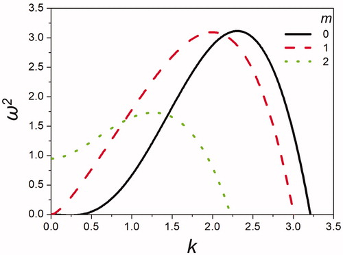
Figure 8. Effect of the charging level (Γ_e) on the most dominant wavelength (λ) for various modes m at b/a = 5.

3. Frequency of oscillation for a cylindrical jet

For a column that is distorted and then allowed to relax, surface tension causes the column to oscillate over time, presuming a low charge level. However, for a high charge level, the column bifurcates. Thus, we begin with assumed distortion shapes (various modes) and solve the linear problems in order to investigate the frequency or period of the electrified liquid oscillation.

In the previous section, the growth rate was discussed; here, the frequency of oscillation (the imaginary part of in Equation (1)(1) ) is introduced. We presume a sinusoidal oscillation of mode number m in a liquid column that is distorted slightly from a perfect cylinder in order to investigate the stability and periodic oscillations of the column.

In order to derive the velocity potential , the surface shape is set as (54) where (55)

The velocity potential is governed by the 2D Laplace equation in cylindrical coordinates: (56)

We assume the solution of the velocity potential of: (57)

Equation (57)(57) is substituted into (56)(56) to obtain, (58)

This yields (59) and (60)

Equation (59)(59) has a solution of the form . However, the solution must be finite at r = 0. Thus, B must be equal to 0. Then, (61)

Equation (60)(60) has a solution of the form . However, is only present in the argument of the cosine function (see Equation (55)(55) ). Thus, D is set to 0. Then, (62)

Rewriting Equation (57)(57) and absorbing the constants A and C into the function T(t) yields (63)

Applying the kinematic condition at the surface and using Equation (55)(55) gives: (64)

Then Equation (63)(63) becomes (65)

In order to derive the electrostatic potential , we assume the solution of (66)

The electrostatic potential is also governed by Laplace’s equation. (67)

Equation (66)(66) is substituted into (67)(67) to obtain (68)

This yields (69) and (70)

Equation (69)(69) is solved as (71)

Equation (70)(70) has a solution of the form . However, is only present in the argument of the cosine function (see Equation (54)(54) ). Thus, D is set to 0. Then, (72)

Now Equation (66)(66) is rewritten with a new constant K. The constants A, B, and C are absorbed into the function T_e(t) and the constant K. (73)

The boundary condition at r = b (the ground location) is used to evaluate K. (74)

The boundary condition at the surface (r_s) is used to evaluate T_e(t). (75) (76)

We substitute Equations (75)(75) into (76)(76) and T_e(t) becomes (77)

Equation (73)(73) is rewritten as (78)

We must introduce Bernoulli’s equation from Equations (30)(30) through (35)(35) and (37)(37) to obtain an equation for the frequency of oscillation. The surface curvature for this problem is (79)

In order to express Equation (35)(35) , the boundary conditions are applied at the surface and Equation (78)(78) is differentiated. (80)

Equation (54)(54) is substituted for r_s and Equation (80)(80) is linearized as (81)

Equation (81)(81) is substituted into (35)(35) and the higher-order terms are neglected, yielding (82)

For the right-hand side of Equation (31)(31) , , Equation (32)(32) is subtracted from Equation (33)(33) and Equations (37)(37) and (82)(82) are substituted in. (83)

We must differentiate the velocity potential given as Equation (65)(65) with respect to time t in order to express at the surface (linearization at ): (84)

Substituting Equation (83)(83) and (84)(84) into (31)(31) yields the frequency of oscillation : (85)

Every dimensional term is denoted by ()′. Equations (50)(50) and (52)(52) are substituted in to nondimensionalize Equation (85)(85) . This yields our final nondimensional result. (86)

We introduce the new parameters of , the ratio a/b raised to the power 2 m, and Q_c, the total dimensionless charge on the cylinder: (87) (88)

Then Equation (86)(86) becomes (89)

For ground locations near the charged cylinder (b → a), approaches 1, which makes in Equation (89)(89) . The cylinder is thus unconditionally unstable in this case. However, as b → ∞, Equation (89)(89) converges to Rayleigh’s nondimensionalized result, presented below: (90)

The frequency depends on the mode number m and the point charge Q_c (in terms of the dimensionless charge level Γ_e). Regardless of m, Γ_e can be made sufficiently large to cause to become negative; thus, it contributes to the growth rate. At this point, the electrostatic pressure exceeds the capillary pressure and the column becomes unstable.

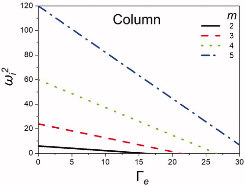
Figure 9 shows the square of the frequency of oscillation (ω_i²) for varied electrostatic strengths and various modes (m = 2, 3, 4, and 5) of a cylindrical jet. As Γ_e is increased, the frequency of oscillation decreases for all modes. In general, the surface tension force contributes to increases in oscillation, because the surface tension responds quickly to perturbations and induces high-rate system oscillation. Meanwhile, the opposing electrostatic force slows the oscillation excited by surface tension. Thus, greater electrostatic strengths correspond to lower-frequency oscillations, as indicated in Figure 9 for all modes.

Figure 9. Effect of the charging level Γ_e on the frequency of oscillation squared ω_i² for various modes m of a cylindrical jet at b/a = 10.

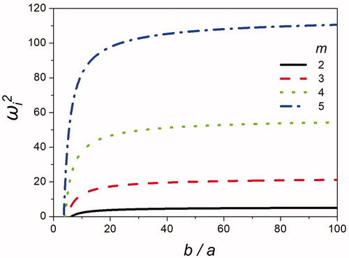
Figure 10 shows the square of the frequency of oscillation (ω_i²) for varied ground locations, which determine the strength of the electric field, for various modes (m = 2, 3, 4, and 5). As the ground location (b/a) distance is increased, the electric field strength decreases and eventually approaches zero, which is equivalent to the case in which Γ_e = 0. Therefore, the value of ω_i² converges to the value observed at Γ_e = 0 in Figure 9.

Figure 10. Effect of the ground location b/a or electric field on the frequency of oscillation squared ω_i² for various modes m of a cylindrical jet at Γ_e = 10.

4. Frequency of oscillation for a spherical droplet

Here, the surface shape of the droplet is defined as (91) where . The droplet potential is governed by the Laplace equation in spherical coordinates (see Yih 1969): (92)

Using the separation of variables technique presented in Section 3, we obtain the velocity potential for the droplet. (93)

Similarly, the electrostatic potential is also obtained; satisfies the boundary conditions of at and at . (94)

The pressure balances in the unperturbed and perturbed regions can be written as (where for the sphere in the unperturbed region): (95) (96) where (97) (98) (99)

We recall and differentiate it with respect to r. This yields (100) and therefore: (101)

Equation (94)(94) is differentiated with respect to r in order to express P_e in Equation (96)(96) : (102) and the higher-order terms are neglected. (103)

Binomial expansion gives (104) and (105)

Equations (104)(104) and (105)(105) are substituted into (103) and again the higher-order terms are neglected: (106)

Therefore, the pressure at the interface is: (107)

Equation (93)(93) is differentiated with respect to time and evaluated at in order to relate it to Bernoulli’s equation (see Equation (31)(31) ). (108)

Equations (101)(101) and (107)(107) are substituted with (99)(98) and (108)(108) into Equation (31)(31) to obtain: (109)

We denote dimensional terms as ( )′ and use Equations (50)(50) and (52)(52) to nondimensionalize Equation (109)(109) . The final nondimensional result is: (110)

This is in agreement with Rayleigh’s (1882) result.

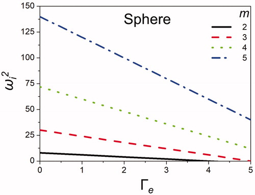
Figure 11 shows the square of the frequency of oscillation (ω_i²) with varying electrostatic strength for the various modes m = 2, 3, 4, and 5 of a spherical droplet. Higher modes show greater frequencies of oscillation. As Γ_e is increased, the frequency of oscillation decreases for all modes. The surface tension force contributes to increasing oscillation frequency, while the electrostatic force slows the oscillation in competition against the surface tension.

Figure 11. Effect of the charging level Γ_e on the frequency of oscillation squared ω_i² for various modes m of a spherical droplet.

5. Conclusion

A complete derivation is provided for the instability analysis of an electrified jet and droplet. The dispersion equation was derived to identify the most dominant wavelength of instability oscillation at various charging levels. As the charging level was increased, the dominant wavelength decreased. For the charging level of zero, the dispersion equation yielded the result of Rayleigh’s nonelectrified jet of ka = 0.69 or λ = 9a. The dispersion equation was also consistent with those of Melcher (1963), Taylor (1969), and Neukermans (1973).

Regarding the frequency of oscillation, the complete relations for an electrified cylindrical jet and spherical droplet were derived. The derivation of the electrified cylindrical jet was provided for the first time, as Rayleigh did not provide details for this case. The expression derived herein included the effects of electric field strength, which were not addressed by Rayleigh. We performed various parametric studies to show the effects of variations in charge levels and electric field strengths. These detailed derivations and final expressions will be of interest to scientists and engineers who work in the widespread fields in which electrified jets are applied.

Disclosure statement

No potential conflict of interest was reported by the authors.

Additional information

Funding

This work was supported by the National Research Council of Science & Technology (NST) grant by the Korea Government (MSIP) (No. CRC-16-02-KICT). This research was supported by the Technology Development Program to Solve Climate Changes of the National Research Foundation (NRF) funded by the Ministry of Science, ICT & Future Planning (NRF-2016M1A2A2936760), NRF-2013R1A5A1073861, and NRF-2017R1A2B4005639.

References

- Artana, G., H. Romat, and G. Touchard. 1998. Theoretical analysis of linear stability of electrified jets flowing at high velocity inside a coaxial electrode. J. Electrostatics 43 (2):83–100.
- Basset, A. B. 1894. Waves and jets in a viscous liquid. Amer. J. Mathematics 16 (1):93–110.
- Collins, R. T., M. T. Harris, and O. A. Basaran. 2007. Breakup of electrified jets. J. Fluid Mechanics 588:75–129.
- Hendricks, C., and J. Schneider. 1963. Stability of a conducting droplet under the influence of surface tension and electrostatic forces. Amer. J. Physics 31(6):450–3.
- Li, F., X.-Y. Yin, and X.-Z. Yin. 2005. Linear instability analysis of an electrified coaxial jet. Phys. Fluids 17 (7):077104.
- Lopez-Herrera, J. M., A. M. Gañán-Calvo, and M. Perez-Saborid. 1999. One-dimensional simulation of the breakup of capillary jets of conducting liquids. Application to E.H.D. spraying. J. Aerosol Sci. 30 (7):895–912.
- Melcher, J. R. 1963. Field-coupled surface waves. Cambridge: MIT.
- Neukermans, A. 1973. Stability criteria of an electrified liquid jet. J. Appl. Phys. 44 (10):4769–70.
- Rayleigh, L. 1878. On the instability of jets. Proc. London Math. Soc. 10 (1):4–13.
- Rayleigh, L. 1882. XX. On the equilibrium of liquid conducting masses charged with electricity. Philosoph. Mag. Ser. 14 (87):184–6.
- Schneider, J., N. Lindblad, C. Hendricks, Jr, and J. Crowley. 1967. Stability of an electrified liquid jet. J. Appl. Phys. 38 (6):2599–605.
- Setiawan, E., and S. Heister. 1997. Nonlinear modeling of an infinite electrified jet. J. Electrostat. 42 (3):243–57.
- Taylor, G. 1964. Disintegration of water drops in an electric field, in proceedings of the royal society of London A: Mathematical, physical and engineering sciences. Roy. Soc. 280 (1382):383–97.
- Taylor, G. 1969. Electrically driven jets, in proceedings of the royal society of London A: Mathematical, physical and engineering sciences. Roy. Soc. 313 (1515):453–75.
- Wangsness, R. K. 1986. Electromagnetic fields. New York: Wiley-VCH.
- Watson, G. 1922. Theory of Bessel functions. Cambridge: Cambridge Press.
- Yih, C. 1969. Fluid mechanics: A concise introduction to the theory. New York, NY: McGraw-Hill.