Thermal/optical reflectance equivalent organic and elemental carbon determined from federal reference and equivalent method fine particulate matter samples using Fourier transform infrared spectrometry

Abstract

A fine particulate matter (PM_2.5) monitoring network of filter-based federal reference methods and federal equivalent methods (FRM/FEMs) is used to assess local ambient air quality by comparison to National Ambient Air Quality Standards (NAAQS) at about 750 sites across the continental United States. Currently, FRM samplers utilize polytetrafluoroethylene (PTFE) filters to gravimetrically determine PM_2.5 mass concentrations. At most of these sites, sample composition is unavailable. In this study, we present the proof-of-principle estimation of the carbonaceous fraction of fine aerosols on FRM filters using a nondestructive Fourier transform infrared (FT-IR) method. Previously, a quantitative FT-IR method accurately determined thermal/optical reflectance equivalent organic and elemental carbon (a.k.a., FT-IR organic carbon [OC] and elemental carbon [EC]) on filters collected from the chemical speciation network (CSN). Given the similar configuration of FRM and CSN aerosol samplers, OC and EC were directly determined on FRM filters on a mass-per-filter-area basis using CSN calibrations developed from nine sites during 2013 that have collocated CSN and FRM samplers. FRM OC and EC predictions were found to be comparable to those of the CSN on most figures of merit (e.g., R²) when the type of PTFE filter used for aerosol collection was the same in both networks. Although prediction accuracy remained unaffected, FT-IR OC and EC determined on filters produced by a different manufacturer show marginally increased prediction errors suggesting that PTFE filter type influences extending CSN calibrations to FRM samples. Overall, these findings suggest that quantifying FT-IR OC and EC on FRM samples appears feasible.

© 2018 American Association for Aerosol Research

EDITOR:

• Pramod Kulkarni

1. Introduction

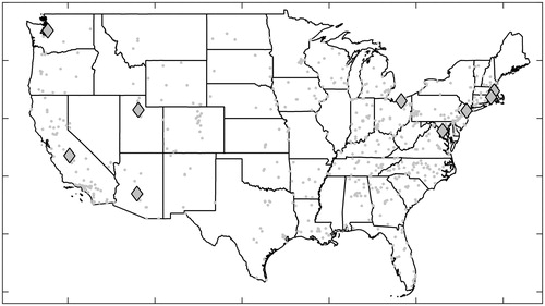
Ambient fine aerosol (a.k.a., PM_2.5) describes atmospheric particulate matter with an aerodynamic diameter of less than 2.5 μm (Wilson et al. 2002). Given its negative health consequences and association with visibility reduction (Anderson, Thundiyil, and Stolbach 2012; Brook et al. 2010; Pope and Dockery 2006; Watson 2002), provisions in the Clean Air Act empower the United States Environmental Protection Agency (EPA) to specify and enforce National Ambient Air Quality Standards (NAAQS) for PM_2.5 (Section 109, 42 U.S.C. 7409). The PM_2.5 monitoring network includes three components: a network of 24-h filter-based federal reference and equivalent methods (FRM/FEMs) used not only for comparison to the NAAQS; continuous monitors used primarily for public reporting of the Air Quality Index—but also for comparison to the NAAQS when continuous FEMs are employed; and speciation samplers operated as part of the chemical speciation network (CSN) and Interagency Monitoring of PROtected Visual Environments (IMPROVE) program used to characterize the chemical composition comprising PM_2.5 (Solomon et al. 2014). The Code of Federal Regulations (40 CFR, Part 50, Appendix L) provides guidelines to gravimetrically determine PM_2.5 mass-concentrations (µg/m³) from polytetrafluoroethylene (PTFE) filters (Noble et al. 2001). There are currently about 950 filter-based and continuous FRM/FEM monitors in the PM_2.5 network. In 2013, filter-based FRM/FEM monitoring occurred at nearly 750 sites across the continental United States (Figure 1). The term “FRM/FEM” will be shortened to “FRM” throughout the remainder of the document given that samples from the nine sites used in this study are derived from 24-h filter measurements only.

Figure 1. FRM samplers located across the continental United States in 2013. The nine sites considered in this study are identified with diamonds. Air Quality System (AQS) site identifications and other sample information is located in online SI (e.g., Figure S1).

Adopting nondestructive speciation techniques, such as those based on Fourier transform infrared (FT-IR) spectroscopy, into existing FRMs may serve to expand the scope of epidemiology studies, lead to more targeted aerosol-source abatement strategies, and potentially result in updated and improved NAAQS. Specifically, several mechanisms have been proposed associating the particle size, particle number, shape, and chemical composition of PM_2.5 to biological response and toxicity (Valavanidis, Fiotakis, and Vlachogianni 2008). For example, constituents associated with the organic carbon (OC) fraction of fine aerosol (e.g., quinones, polycyclic aromatic hydrocarbons) have been linked to the generation of reactive oxygen species that damage the lungs via oxidative stress (Nel 2005). A recent meta-analysis also found a positive association between short term exposure to elemental carbon (EC) and increases in all-cause and cardiopulmonary mortality (Atkinson et al. 2015). Along with black carbon—similar to the EC determined from thermal analysis (Andreae and Gelencsér 2006; Salako et al. 2012)—current research focuses on that a fraction of light absorbing OC species (a.k.a., brown carbon) that compromise visibility and increase the radiative forcing of fine aerosols (Bond et al. 2013; Laskin, Laskin, and Nizkorodov 2015). Evaluating the feasibility of determining FRM OC and EC using FT-IR spectrometry therefore provides a first step in understanding of extent and limitations of integrating nondestructive speciation techniques into FRMs.

Quantifying OC and EC via the FT-IR analysis of PTFE filters (a.k.a., FT-IR OC and EC) has been demonstrated in several studies using samples from two US monitoring networks (Dillner and Takahama 2015a, 2015b; Reggente, Dillner, and Takahama 2015; Takahama and Dillner 2015; Weakley, Takahama, and Dillner 2016; Weakley et al. 2018). Specifically, PTFE filters are analyzed using FT-IR transmission spectroscopy with the resulting spectra calibrated to thermal/optical reflectance (TOR) OC or EC measured on collocated quartz filters. These studies establish FT-IR OC and EC as determinable in urban samples from the CSN (2013 sampling year) as well as rural samples from the IMPROVE network (2011 and 2013 samples). CSN studies demonstrate that OC and EC are quantifiable using FT-IR transmission spectra acquired from very low areal density ambient samples (∼2 µg-OC/cm² and ∼1 µg-EC/cm²). Aerosol sources appear to impact CSN EC predictions to a measurable extent, motivating the development of a multilevel modeling scheme to distinguish and then determine “typical” and “atypical” CSN EC (where the atypical EC was found to describe diesel particulate matter). IMPROVE network studies indicate that FT-IR methods are reasonably robust, that is, OC and EC are quantified on filters collected from different IMPROVE sites and sampling years not considered (“seen”) by the original calibration. Given the FT-IR method’s robustness, very similar configuration of CSN and FRM aerosol samplers, and the requirement that FRM samples be stored cold for 1-2 years before archiving, enables a straightforward extension of CSN OC and EC calibrations to FRM filters.

This study presents a first endeavor exploring the broader implication of extending FT-IR calibrations (CSN) to filter samples collected in a different sampling network (FRM). Specifically, CSN OC and EC calibrations are first developed using samples from nine geographically-diverse sites (see Figure 1, diamonds). Calibration parameters (i.e., regression coefficients) are next applied to the FT-IR spectra of collocated FRM filters to determine FRM OC and EC. FRM OC and EC predictions are then compared to CSN predictions on several figures of merit (e.g., R² and bias), calculated by comparing FT-IR OC and EC predictions to TOR references values (from the CSN). Since FRM samples were collected on two types of PTFE filters (Measurement Technology Laboratories (MTL) and Whatman™), and CSN samples were collected on Whatman™ PTFE filters alone, a controlled investigation links FRM prediction errors to the type of filter used for aerosol collection. Specifically, the different filter media used to collect most samples in the FRM network (MTL) confer spectral interferences distinct from CSN filters (Whatman) on the prediction problem. Therefore, we introduce the use of 95% bootstrapped confidence intervals on figures of merit to formally evaluate the impact of filter type.

2. Methods

2.1. Aerosol sampling in the CSN and FRM

Nine CSN sites situated in or around Boston, MA, Cleveland, OH, Elizabeth, NJ, Fresno, CA, Phoenix, AZ, Providence, RI, Salt Lake City, UT, Seattle, WA, and Washington, DC were considered in this study. Ambient aerosol was collected on both Whatman™ 46.2 mm PTFE membrane filters and Pall™ 25 mm quartz fiber filters every third day during 2013 at each CSN site. Ambient air was sampled through PTFE filters using the SASS speciation samplers configured at a real flow rate of 6.7 L/min (www.metone.com). Furthermore, URG-3000N samplers aspirated ambient air through quartz fiber filters at 22.0 L/min (www.urgcorp.com). Following aerosol collection, samples were shipped and stored cold for further analysis (4 °C).

FRM samplers are configured to collect ambient air at a volumetric flow rate of 16.7 L/min through 46.2 mm PTFE filters meeting the design specifications in 40 CFR, part 50, Appendix L. Whatman™ PTFE filters meeting these specifications were used for aerosol collection at Fresno, CA during the full duration of 2013. Samples collected on Whatman™ (www.gelifesciences.com) filters at Phoenix, AZ spanned January 1, 2013 to June 6, 2013. MTL PTFE membrane filters (www.mtlcorp.com) were used for the remaining part of 2013 at Phoenix, AZ. Field samples from the remaining sites were collected exclusively on MTL filters. Overall, 2,400 FRM filters from the nine sites considered in this study were available for FT-IR analysis.

2.2. Thermal/optical and FT-IR analysis

TOR OC and EC were speciated from quartz fiber filters at the Desert Research Institute (Reno, NV) using the IMPROVE_A thermal/optical reflectance protocol (Chow et al. 2007). The EPA’s Air Quality System (AQS) database was accessed on July 27, 2015 to retrieve TOR OC and EC quartz filter data (http://aqsdr1.epa.gov/aqsweb/aqstmp/airdata/). TOR OC and EC values were artifact corrected by subtracting the median monthly field blank OC and EC concentration from each sample. TOR measurements were then converted from mass-concentration (µg/m³) to a mass-per-area basis (µg/cm²) prior to FT-IR calibration by taking into account the total volume of air sampled over 24-h (m³) and the true deposit area (11.3 cm²) of PTFE filters (McDade, Dillner, and Indresand 2009)—the reasons for which are discussed in Section 2.3.

FT-IR transmission spectra were collected from PTFE filters at the Air Quality Research Center (AQRC, Davis, CA) using the Bruker Tensor 27 FT-IR spectrometer (Bruker Optics, Billerica, MA) equipped with a liquid nitrogen cooled mercury-cadmium-telluride detector. Spectral resolution was specified at 4 cm⁻¹ over a spectral range of 4,000 to 400 cm⁻¹ (2.5–24 µm). Additional details as to FT-IR collection can be found in Ruthenburg et al. (2014). Overall, 915 CSN samples, including 30 field blanks, were available for FT-IR OC and EC calibration and validation.

2.3. CSN OC and EC calibration and extension to FRM filters

Extending CSN OC and EC calibrations to FRM filter samples is straightforward on a mass-per-unit area (areal density) basis, as conventionally done for beta attenuation monitoring measurements (Jaklevic et al. 1981). Formally, this amounts to first calibrating CSN spectra to TOR OC (or EC) areal densities then simply applying the estimated partial least-squares (PLS) regression coefficients to FRM spectra as (1) where denotes an m-length vector of predicted OC (or EC) areal densities (in µg/cm²), are the FRM spectra (), the -length vector of PLS regression parameters, and the model’s intercept (Wold, Sjöström, and Eriksson 2001). Unlike , the subscript “CSN” was not included on and nor since these parameters generalize, in principle, to both CSN and FRM samples when the dependent variable is posed in terms of areal density.

On an areal density basis, with all other factors remaining fixed or negligible, the amount of aerosol measured on CSN filters should differ from collocated FRM filters by the ratio of CSN and FRM sampling volumetric flow rates (6.7 L/min / 16.7 L/min =0.4). Therefore, when evaluating OC and EC predictions against collocated TOR measurements (), as an error () in units of mass concentration (µg/m³), as (2) one must ensure that predicted areal densities () are converted to mass-concentrations and then scaled using the flow rate ratio.

2.4. Sample partitioning: Overall performance and inferring a filter effect

Identical to previous work (Weakley, Takahama, and Dillner 2016; Weakley et al. 2018), CSN samples are sorted by AQS site code and date (ABCD_MMDDYYYY) with TOR measurements and spectra allocated to either a calibration (model training) or test (validation) set. The calibration set describes those samples used to estimate regression parameters () while the test set is used to validate CSN OC and EC predictions. Partitioning sorted samples into a calibration and test set is performed by placing every third sorted sample in the test set. This form of stratified partitioning attempts to capture the factors effecting aerosol composition, such as seasonality and source disparities between sites, equally well in both the calibration and test sets (Dillner and Takahama 2015a, b). Table 1 summarizes the number of samples contained in the calibration, test, and FRM prediction sets. Samples are further distinguished in terms of the filter type used for aerosol collection.

Table 1. FT-IR calibration, method testing, and FRM prediction samples distinguished by network, filter type, and field status (sampled vs. blank).

Network	Set	Filter type	Sampled	Blank
CSN	Calibration	Whatman	587	20
CSN	Test	Whatman	329	10
FRM	Prediction	MTL	563	81
FRM	Prediction	Whatman	138	22

Although ∼2,400 FRM spectra have been measured at the AQRC, Equation (2) limits the number of FRM samples considered in this study. Specifically, Figure 2 shows the TOR data available to evaluate FRM OC and EC predictions by Equation (2). TOR data have also been partitioned according to their role in CSN model training and validation, creating four intersections between CSN calibration and test samples with FRM MTL and FRM Whatman samples. Overall, 138 Whatman (92 + 46) and 563 MTL (365 + 198) samples are available for FRM evaluation given a corresponding availability of TOR data (all intersections; N = 701). Analyses related to these data sets are provided in Tables 2 and 3 as well as illustrated in Figures 2 and 3.

Figure 2. Illustration of the data available for CSN and FRM analysis as distinguished by sample network (CSN vs. FRM), study role (calibration vs. test set), or filter type (MTL vs. Whatman). Intersections symbolize the maximum number of TOR data available for FRM OC and EC evaluation. For example, of the 470 FRM Whatman filters collected, only 92 TOR samples are available for FRM OC and EC evaluation and for CSN calibration upper as shown in the upper left intersections in both diagrams (red–yellow). Another 46 TOR samples are available for FRM OC and EC evaluation and for CSN testing as shown in the upper right intersections in both diagrams (red–green). Field blanks are not considered here as no aerosol carbon is present.

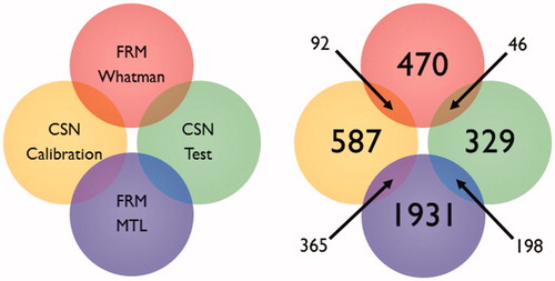
Figure 3. FRM OC predictions plotted against TOR OC reference concentrations. FT-IR OC predictions are first pooled (a = MTL + Whatman) and then distinguished by filter type (b = MTL, c = Whatman). Predicted OC areal densities are converted to the more familiar mass-concentrations (µg/m³) here.

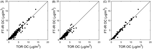
Table 2. FT-IR OC determined on FRM filters compared to the base case CSN OC from Weakley et al. (2016).

Network, filter	N	Range (µg/cm^2)	R^2	Bias (%)	Normalized error (%)	% below MDL
CSN Whatman (base case)	329 (10)	0–7.2 (0%)	0.955 (0.952, 0.957)	2.9 (1.2, 5.1)	9.1 (8.8, 10.0)	0.6 (0.0, 0.6)
FRM MTL + Whatman	701 (103)	0–17.8 (4.4%)	0.939 (0.933, 0.942)	1.7 (0.0, 4.0)	13.7 (13.2, 14.7)	0.4 (0, 0.4)
FRM MTL	563 (81)	0–11.5 (1.8%)	0.884 (0.870, 0.893)	1.7 (–0.4, 4.1)	14.7 (13.9, 15.8)	0 (0, 0)
FRM Whatman	138 (22)	0–17.8 (15.2%)	0.969 (0.969, 0.977)	2.2 (–0.9, 5.8)	10.3 (9.5, 12.1)	0 (0, 0)

Upper and lower confidence intervals for figures of merit are contained in parentheses where appropriate. Sample number (N) denotes only nonblank samples with blank sample number provided directly below them in parentheses. The calibration range (µg/cm²) and percentage of samples falling outside the range of the CSN Whatman (base case) calibration are shown, the later directly below reported ranges in parentheses.

Table 3. FT-IR EC determined on FRM filters compared to the base case CSN EC from Weakley et al. (2018).

Network, filter	N	Range (µg/cm^2)	R^2	Bias (%)	Normalized error (%)	% below MDL
CSN Whatman (base case)	329 (10)	0–1.9 (0%)	0.884 (0.861, 0.885)	2.2 (–1.2, 6.7)	19.2 (18.9, 22.8)	4.8 (1.7, 13.2)
FRM (MTL + Whatman)	701 (103)	0–4.8 (10.7%)	0.760 (0.569, 0.777)	5.6 (–1.6, 13.1)	30.5 (28,2, 34.8)	31.8 (11.4, 57.2)
FRM MTL	563 (81)	0–4.7 (17.6%)	0.694 (0.429, 0.726)	7.8 (–2.6, 16.9)	32.8 (30.0, 38.9)	35.8 (9.3, 64.7)
FRM Whatman	138 (22)	0–4.8 (9.0%)	0.886 (0.826, 0.900)	3.3 (–5.8, 12.6)	18.1 (17.7, 25.8)	11.0 (8.1, 21.3)

Upper and lower confidence intervals on figures of merit are contained in parentheses where appropriate. Sample number (N) considers only nonblank samples with blank samples listed directly below them in parentheses. The calibration range (in µg/cm²) and percentage of samples falling outside the CSN Whatman (base case) calibration range are shown, the later directly below reported ranges in parentheses.

Of the 215 unmatched TOR samples (= [916 available TOR samples] – [701 matched FRM filters]), 65 TOR measurements were likely unmatched to FRM filters totally-at-random (e.g., FRM filter missing due to sampler error, damaged, or lost). Tables S1 and S2 of online supplementary information provides details as to reasons for the lack of matching for the remaining 141 filters as well as details about the additional 1,554 FRM filters that did not have TOR data.

Inferring whether filter type influences OC and EC predictions requires applying additional restrictions on the number of FRM and CSN samples compared to control for possible statistical confounds. First, samples in the intersections between FRM and CSN calibration samples (Figure 2, yellow) should not be considered when assessing FRM OC and EC predictions since calibration-set samples falsely bias CSN figures of merit favorably, potentially overstating the negative effect of MTL filter type on OC and EC predictions. Second, the prediction quality of field blanks should not be considered, even though TOR data are not required for evaluation by Equation (2), since most FRM blanks cannot be matched exactly by site and date to CSN samples (see Table 1). In other words, any error-variance related to predictions garnered from unmatched field blanks is not necessarily linked to the filter effect under investigation. Analogous to matched case-control studies only the 46 FRM Whatman filters and 198 FRM MTL filters are matched and compared to their respective CSN Whatman filters (Gamble 2014). These samples correspond to the upper right (red-green) and lower right (purple-green) intersections in both diagrams in Figure 2. The results of this analysis are provided in Table 4.

Table 4. Matched CSN and FRM OC and EC comparisons according to the scheme presented in Figure 2.

Network, filter	N	Range (µg/cm^2)	R^2 (OC)	Bias (% OC)	Normalized error (% OC)	Range (µg/cm^2)	R^2 (EC)	Bias (% EC)	Normalized error (% EC)
CSN Whatman	46	0–7.2 (0%)	0.975 (0.971, 0.977)	4.6 (1.4, 7.6)	9.0 (7.9, 11.5)	0–1.9 (0%)	0.949 (0.923, 0.955)	2.6 (–6.9, 8.5)	14.3 (13.1, 21.8)
FRM Whatman	46	0–17.8 (15.2%)	0.963* (0.955, 0.967)	–0.1 (–3.6, 3.3)	8.2 (7.2, 10.0)	0–4.3 (21.7%)	0.936 (0.888, 0.952)	–3.2 (–11.4, 5.1)	14.0(9.6, 18.3)
CSN Whatman	198	0–7.2 (0%)	0.935 (0.924, 0.938)	3.3 (1.3, 5.0)	9.0 (9.0, 11.0)	0–1.9 (0%)	0.770 (0.690, 0.773)	1.1 (–5.0, 6.9)	22.2 (21.6, 27.6)
FRM MTL	198	0–11.5 (2.0%)	0.850* (0.824, 0.866)	0.0 (–2.3, 2.4)	11.8* (10.8, 12.9)	0–4.0 (8.2%)	0.582* (0.114, 0.625)	–0.1 (–10.5, 7.4)	28.2 (23.3, 33.8)

Forty-six CSN Whatman and CSN FRM samples (rows 1 and 2) and 198 CSN Whatman and FRM MTL samples (rows 3 and 4) are site-date matched exactly and compared to control for potential inference confounds, respectively. The calibration range (in µg/cm²) and percentage of samples falling outside the CSN Whatman (base case) calibration range are shown in parentheses.

2.5. Spectra processing

CSN OC and EC calibrations are developed after transforming FT-IR absorption spectra to second derivative spectra using a second order, 20-point, Savitsky–Golay filter (Savitzky and Golay 1964). Derivative transformation is considered the most straightforward approach to minimizing secondary optical effects in the infrared spectra; namely, the scattering of infrared radiation by the PTFE fibers. Scattering presents itself in infrared spectra as a broad baseline between ∼4,000 and 1,300 cm⁻¹ and is effectively suppressed by derivative transformation. Furthermore, instead of using all wavenumbers for calibration (=2,764 discrete measurements spanning 4,000–400 cm⁻¹) the backward Monte Carlo unimportant variable elimination (BMCUVE) method was used to prune redundant wavenumbers from the CSN spectra and then the FRM spectra (Weakley et al. 2014). Previous work has shown that BMCUVE tends to remove wavenumbers corresponding to useless background and filter absorption, generally improving prediction accuracy as a result (Weakley, Takahama, and Dillner 2016; Weakley et al. 2014, 2018). Spectra resulting from derivative filtering and wavenumber selection are herein referred to as processed FT-IR spectra.

2.6. Comparing CSN and FRM OC and EC predictions

CSN OC and EC are determined per procedures presented in Weakley, Takahama, and Dillner (2016) and Weakley et al. (2018), respectively. Only the essential operations in either calibration protocol are presented here. For both OC and EC calibrations, processed spectra (from the calibration set) are calibrated to corresponding TOR measurements using the nonlinear iterative partial least squares (NIPALS) algorithm (Wold, Sjöström, and Eriksson 2001). A minimized root-mean-square error of fivefold cross-validation determines the number of PLS components to use for modeling (Arlot and Celisse 2010). For OC, one set of regression coefficients are estimated. For EC, the multilevel modeling scheme generates two sets of regression coefficients for “typical” and “atypical” samples.

FT-IR OC and EC are determined from Equation (1) using CSN test spectra and then FRM spectra. Equation (2) provides the errors necessary to calculate figures of merit to ascertain the validity of CSN predictions and ability to extend the calibration to FRM samples. Figures of merit considered in this study include the coefficient of determination (R²), concentration-normalized bias, normalized error, and the percentage of predicted samples falling below the MDL. In this study, the term “accuracy” concerns normalized bias and the term “precision” concerns metrics derived from regression standard errors such as R² and normalized error.

FRM OC and EC predictions are judged valid if predictions are comparable to the best “base case” CSN predictions developed in previous work (Weakley, Takahama, and Dillner 2016; Weakley et al. 2018). Concerning the effect of filter type in particular, we hypothesize that additional bias and error may be introduced into FRM MTL predictions given that CSN Whatman filters are used for calibration. The effect of filter type was therefore assessed using 95% bootstrapped confidence intervals for CSN and FRM figures of merit. The null hypothesis is not rejected (e.g., no difference in CSN and FRM OC predictions according to R²) if either FRM or CSN confidence intervals capture the test statistic (e.g., R² value) of the other. The null hypothesis is rejected if the contrary occurs.

2.7. Analysis software

The Matlab™ base and signal processing toolbox was used for most data manipulation and visualization purposes (2016b, The MathWorks, Inc., Natick, MA, USA). The NIPALS algorithm and single-pass MCUVE filter function were available from the open-source libPLS package (v1.9, Changsha Nice City, China). BMCUVE wavenumber selection was programed by the authors.

3. Results and discussion

Table 2 compares FRM OC predictions to CSN OC figures of merit taken from Weakley, Takahama, and Dillner (2016). First, without distinguishing between PTFE filter type, we see that FRM OC predictions (N = 701) appear comparable to the CSN Whatman (base case) suggesting that CSN OC models are extendable to FRM filters. Separating FRM OC predictions according to filter manufacturer provides a preliminary indication that MTL predictions (N = 563) are somewhat less precise (lower R², higher normalized error) than FRM Whatman predictions (N = 138). This is illustrated in Figure 3b and c which show greater scatter in FRM MTL predictions than FRM Whatman predictions when compared to TOR. Additionally, normalized FRM errors are all elevated relative to the CSN Whatman (base case). For FRM Whatman predictions in particular, this may have resulted from extrapolation errors where 15.2% of the samples fall outside the range of the original calibration (in µg/cm²). Notably, FRM predictions exhibit no significant changes in bias relative to the CSN Whatman (base case; p < 0.05) and, in fact, are unbiased according to confidence intervals spanning 0% bias. Unbiased FRM predictions also provide evidence that the OC sampling artifacts—particularly negative (volatilization) artifacts—experienced by FRM samples are likely similar to CSN samples, in spite of the higher flow rate of the former (McDow and Huntzicker 1990).

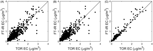
Table 3 and Figure 4 summarize and visualize FRM EC predictions, respectively. Analogous to FRM OC, figures of merit appear diminished for EC predicted on MTL filters with the exception of normalized bias—which is not significantly elevated according to confidence intervals (p < 0.05). Figure 4b and c again shows that FRM Whatman predictions show minimal scatter relative to MTL predictions when compared to TOR. Similar to OC, FRM Whatman and CSN Whatman (base case) predictions do not appear to differ markedly. However, in contrast to OC, uncertainties are large for several MTL EC figures of merit as judged by very large 95% confidence intervals. For example, the percentage of MTL EC samples falling below the estimated MDL falls plausibly between 9.3% and 64.7% whereas the range of FRM Whatman MDLs are comparable to CSN base case estimates.

Figure 4. TOR EC reference mass-concentrations plotted against FRM EC predictions. Predictions are pooled (a = MTL + Whatman) and then distinguished by filter type to aid comparison (b = MTL, c = Whatman). Predicted OC areal densities are converted to the more familiar mass-concentrations (µg/m³) here.

Matching CSN and FRM samples to control for potential confounds confirms that FRM MTL predictions have higher error than FRM Whatman predictions while accuracy likely remains unchanged (Table 4). For R² and possibly EC normalized error, CSN Whatman and FRM MTL figures of merit exhibit nonoverlapping confidence intervals for OC and EC predictions (p < 0.05). Conversely, figures of merit are not significantly different when comparing CSN Whatman to FRM Whatman predictions (p > 0.05), with the exception of a depressed FRM OC R². Again, this may reflect additional extrapolation errors due to determining 15.2% of sample OC outside the original range of the CSN calibration. Overall, these results provide strong evidence that filter type, and not differences in CSN and FRM sampling protocols and procedures, negatively affect our ability to extend CSN calibrations to MTL filters. As a caveat, failing to reject a null hypothesis (i.e., p > 0.05) does not necessarily follow from overlapping confidence intervals (Greenland et al. 2016). Only when at least one confidence interval captures the neighboring statistic being compared may we fail to reject the null hypothesis. For example, EC normalized bias for CSN Whatman and FRM Whatman samples are equal to 2.6% and –3.2%, respectively. Although both statistics are roughly equal in magnitude and opposite sign, we can infer that they are not significantly different since the confidence interval for FRM Whatman captures 2.6% (and vice versa). Alternatively, we cannot arrive at a firm conclusion as to the difference between FRM MTL EC and CSN Whatman EC normalized error, although their intervals overlap, since neither interval captures 28.2% or 22.2%, respectively.

Biases reported in Table 4 suggest that MTL OC and EC predictions are likely as accurate as Whatman predictions. Given that bias statistics estimate the average deviation between the FT-IR and collocated TOR measurements, it should follow that MTL and Whatman spectra do not differ significantly, on average, as well. Figure 5a shows that major differences in scattering (4,000–1,300 cm⁻¹) are evident in the raw (unprocessed) CSN and FRM spectra providing sufficient motivation for processing the FT-IR spectra prior to OC and EC calibration. Processing the FT-IR spectra using second derivatives and wavenumber selection vastly suppresses the influence of scattering on OC and EC quantification and generally brings the average CSN and FRM spectra into agreement (Figure 5b and c). Specifically, we see that variations in FRM second derivative spectra fall well within those of the CSN spectra on the wavenumbers relied upon most strongly for quantification (indicated accordingly). A particularly close correspondence between the average spectra (as well as their 5th and 95th percentiles) is observed in the aliphatic C-H stretching region (3,000–2,800 cm⁻¹; Figure 5b), with the possible exception of the CH₃ antisymmetric stretches (2,960 cm⁻¹) used for EC determination (Coates 2006). Figure 5c indicates a less faithful correspondence between the distribution of CSN and FRM spectra, particularly at 1,630 cm⁻¹. Regardless, because average MTL and Whatman spectra track closely on OC and EC quantitative features it follows that FT-IR prediction biases are very similar.

Figure 5. Average raw CSN Whatman (black) and FRM MTL (red) spectra plotted with their 5th and 95th percentiles (dashes; a). The most important wavenumbers used in the OC and EC calibrations, determined according to a variable importance in projection (VIP) score greater than one (Chong and Jun 2005), are indicated (as gray and blue lines), respectively. The processed Whatman and MTL spectra, in the two most analytically pertinent regions, are plotted to assess any connection between prediction bias and error variance (b, c).

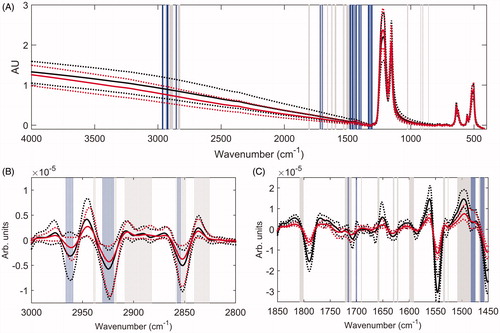
Using Figure 5 as an aid, we speculate that increases in MTL OC and EC prediction errors—as indicated by significantly lower R² and elevated normalized errors statistics—may be tentatively assessed by comparing the distribution (5th and 95th percentiles) of the Whatman and MTL spectra. For example, a poor match between the 5th and 95th percentiles is most evident for the OC and EC calibration at 2,960 and ∼1,500 cm⁻¹, respectively. This may indicate that differences in variability between MTL and Whatman absorption at certain wavenumbers may bear the responsibility for increasing OC and EC prediction error by about +2% OC and +6% EC, respectively.

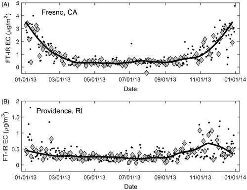
Figures 6 and 7 present time series showing FRM OC and EC determined from two sites: Fresno, CA (Whatman) and Providence, RI (MTL). While it was only possible to validate roughly one-third of these samples using TOR data on account of overlap (see Figure 2), it should be clear from these figures that blind OC and EC predictions (samples with no TOR data) appear consistent with temporal trends derived from validated data. Upon comparing the Providence, RI to Fresno, CA OC time series, the approximate +2% increase in normalized MTL errors is not plainly evident. The same comparison for EC also shows that the approximately +6% increase in Providence, RI errors is not visually apparent (although, the scale of OC and EC concentrations differ by a factor of ∼2 between sites).

Figure 6. Predicted FT-IR OC in Fresno, CA samples (a) and Providence, RI samples (b). Samples validated against available TOR measurements as diamonds (gray) are distinguished from samples with no TOR data (“blinds”; bullets, black). A robust locally weighted error sum-of-squares (LOWESS) smoother was used to estimate the trend line in each series from validated data.

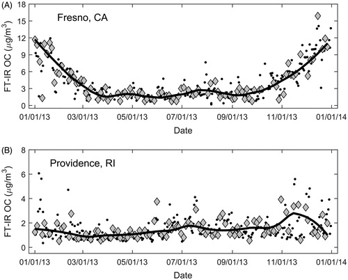
Figure 7. Predicted FT-IR EC in Fresno, CA samples (a) and Providence, RI samples (b). Samples validated against available TOR measurements as diamonds (gray) are distinguished from samples with no TOR data (“blinds”; bullets, black).

4. Conclusions

FT-IR OC and EC have been quantified in atmospheric fine aerosols from nine sites utilizing FRM compliance samplers. First, the FT-IR spectra of CSN fine aerosols (collected on PTFE filters) was calibrated to parallel measurements of TOR OC and EC (speciated from quartz filters) to estimate regression coefficients using a multivariate PLS algorithm. CSN calibrations were then extended to aerosol collected on PTFE filters from FRM samplers providing the nondestructive quantification of FT-IR OC and EC.

FT-IR OC was determined on FRM filters with no loss of accuracy or precision when the type of filter used for aerosol collection matched that used in the CSN (Whatman™ PTFE membrane filters). Additional error (imprecision) was introduced into FRM OC predictions when calibrations were extended to PTFE filters manufactured by the MTL corporation. Matching CSN and FRM samples according to site and date to control for statistical confounds revealed that the type of collection filter used during FRM sampling significantly diminishes OC and EC predictions according to figures of merit. Specifically, increases in normalized error were small, but significant, for OC quantified on MTL filters (+2% normalized error). Notably, OC predictions garnered from FRM samples with MTL filters remained just as accurate as OC determined on FRM Whatman filters (no increase in bias). FT-IR EC was also measured with no loss of accuracy or precision on Whatman PTFE filters collected using FRM samplers. Extending CSN calibrations to MTL filters introduced an additional +6% error in EC predictions but predictions again did not show increased bias.

Overall, FT-IR OC and EC appear quantifiable on FRM compliance samples using CSN calibrations with no loss of accuracy thereby demonstrating primary method feasibility. Future studies may formally investigate the long-run feasibility (robustness) of the FT-IR method applied to FRM samples collected from different sites and years as well as investigate whether calibrating FRM spectra directly to collocated CSN-TOR measurements ameliorates small losses in OC and EC precision linked to filter type.

Acknowledgments

We would like to thank the RTI International team for managing the CSN during the 2013 sampling year. We would also like to thank state personnel for FRM sample collection and handling during the 2013 sampling year.

Disclosure statement

No potential conflict of interest was reported by the authors.

Additional information

Funding

The authors acknowledge funding in cooperation with the U.S. EPA and the IMPROVE program (National Park Service cooperative agreement P11AC91045) and EPFL funding.

References

- Anderson, J. O., J. G. Thundiyil, and A. Stolbach. 2012. Clearing the air: A review of the effects of particulate matter air pollution on human health. J. Med. Toxicol. 8 (2):166–75.
- Andreae, M., and A. Gelencsér. 2006. Black carbon or brown carbon? The nature of light-absorbing carbonaceous aerosols. Atmos. Chem. Phys. 6 (10):3131–48.
- Arlot, S., and A. Celisse. 2010. A survey of cross-validation procedures for model selection. Statist. Surv. 4:40–79.
- Atkinson, R. W., I. C. Mills, H. A. Walton, and H. R. Anderson. 2015. Fine particle components and health—A systematic review and meta-analysis of epidemiological time series studies of daily mortality and hospital admissions. J. Expo. Sci. Environ. Epidemiol. 25 (2):208–214.
- Bond, T. C., S. J. Doherty, D. W. Fahey, P. M. Forster, T. Berntsen, B. J. DeAngelo, M. G. Flanner, S. Ghan, B. Kärcher, D. Koch, et al. 2013. Bounding the role of black carbon in the climate system: A scientific assessment. J. Geophys. Res. Atmos. 118 (11):5380–552.
- Brook, R. D., S. Rajagopalan, C. A. Pope, J. R. Brook, A. Bhatnagar, A. V. Diez-Roux, F. Holguin, Y. Hong, R. V. Luepker, M. A. Mittleman, et al. 2010. Particulate matter air pollution and cardiovascular disease. An update to the scientific statement from American Heart Association. Circulation 121 (21):2331–78.
- Chong, I.-G., and C.-H. Jun. 2005. Performance of some variable selection methods when multicollinearity is present. Chemom. Intell. Lab. Syst. 78 (1–2):103–12.
- Chow, J. C., J. G. Watson, L.-W. A. Chen, M. O. Chang, N. F. Robinson, D. Trimble, and S. Kohl. 2007. The IMPROVE_a temperature protocol for thermal/optical carbon analysis: Maintaining consistency with a long-term database. J. Air Waste Manag. Assoc. 57 (9):1014–23.
- Coates, J. 2006. Interpretation of infrared spectra, a practical approach. In Encyclopedia of analytical chemistry, ed. R. A. Meyers, 1st ed., 1–23. Chichester: John Wiley & Sons, Ltd.
- Dillner, A. M., and S. Takahama. 2015a. Predicting ambient aerosol thermal-optical reflectance (TOR) measurements from infrared spectra: Organic carbon. Atmos. Meas. Tech. 8 (3):1097–109.
- Dillner, A. M., and S. Takahama. 2015b. Predicting ambient aerosol thermal-optical reflectance measurements from infrared spectra: Elemental carbon. Atmos. Meas. Tech. 8 (10):4013–23.
- Gamble, J.-M. 2014. An introduction to the fundamentals of cohort and case-control studies. Can. J. Hosp. Pharm. 67 (5):366–72.
- Greenland, S., S. J. Senn, K. J. Rothman, J. B. Carlin, C. Poole, S. N. Goodman, and D. G. Altman. 2016. Statistical tests, P values, confidence intervals, and power: A guide to misinterpretations. Eur. J. Epidemiol. 31 (4):337–50.
- Jaklevic, J. M., R. C. Gatti, F. S. Goulding, and B. W. Loo. 1981. A .beta.-gage method applied to aerosol samples . Environ. Sci. Technol. 15 (6):680–6.
- Laskin, A., J. Laskin, and S. A. Nizkorodov. 2015. Chemistry of atmospheric brown carbon. Chem. Rev. 115 (10):4335–82.
- McDade, C. E., A. M. Dillner, and H. Indresand. 2009. Particulate matter sample deposit geometry and effective filter face velocities. J. Air Waste Manag. Assoc. 59 (9):1045–8.
- McDow, S. R., and J. J. Huntzicker. 1990. Vapor adsorption artifact in the sampling of organic aerosol: Face velocity effects. Atmos. Environ. Part A 24 (10):2563–71.
- Nel, A. 2005. Atmosphere. Air pollution-related illness: Effects of particles. Science 308 (5723):804–6.
- Noble, C. A., R. W. Vanderpool, T. M. Peters, F. F. McElroy, D. B. Gemmill, and R. W. Wiener. 2001. Federal reference and equivalent methods for measuring fine particulate matter. Aerosol Sci. Technol. 34 (5):457–64.
- Pope, C. A., and D. W. Dockery. 2006. Health effects of fine particulate air pollution: Lines that connect. J. Air Waste Manag. Assoc. 56 (6):709–42.
- Reggente, M., A. M. Dillner, and S. Takahama. 2015. Predicting ambient aerosol thermal-optical reflectance (TOR) measurements from infrared spectra: Extending the predictions to different years and different sites. Atmos. Meas. Tech. Discuss. 8 (11):12433–74.
- Ruthenburg, T. C., P. C. Perlin, V. Liu, C. E. McDade, and A. M. Dillner. 2014. Determination of organic matter and organic matter to organic carbon ratios by infrared spectroscopy with application to selected sites in the IMPROVE network. Atmos. Environ. 86:47–57.
- Salako, G. O., P. K. Hopke, D. D. Cohen, B. A. Begum, S. K. Biswas, G. G. Pandit, Y.-S. Chung, S. A. Rahman, M. S. Hamzah, and P. Davy. 2012. Exploring the variation between EC and BC in a variety of locations. Aerosol Air Qual. Res. 12:1–7.
- Savitzky, A., and M. J. E. Golay. 1964. Smoothing and differentiation of data by simplified least squares procedures. Anal. Chem. 36 (8):1627–39.
- Solomon, P. A., D. Crumpler, J. B. Flanagan, R. K. M. Jayanty, E. E. Rickman, and C. E. McDade. 2014. U.S. National PM2.5 chemical speciation monitoring networks—CSN and IMPROVE: Description of networks. J. Air Waste Manag. Assoc. 64 (12):1410–38.
- Takahama, S., and A. M. Dillner. 2015. Model selection for partial least squares calibration and implications for analysis of atmospheric organic aerosol samples with mid-infrared spectroscopy. J. Chemometr. 29 (12):659–68.
- Valavanidis, A., K. Fiotakis, and T. Vlachogianni. 2008. Airborne particulate matter and human health: Toxicological assessment and importance of size and composition of particles for oxidative damage and carcinogenic mechanisms. J. Environ. Sci. Health C Environ. Carcinog. Ecotoxicol. Rev. 26 (4):339–62.
- Watson, J. G. 2002. Visibility: Science and regulation. J. Air Waste Manag. Assoc. 52 (6):628–713.
- Weakley, A., A. Miller, P. Griffiths, and S. Bayman. 2014. Quantifying silica in filter-deposited mine dusts using infrared spectra and partial least squares regression. Anal. Bioanal. Chem. 406 (19):4715–24.
- Weakley, A. T., S. Takahama, and A. M. Dillner. 2016. Ambient aerosol composition by infrared spectroscopy and partial least-squares in the chemical speciation network: Organic carbon with functional group identification. Aerosol Sci. Technol. 50 (10):1096–114.
- Weakley, A. T., S. Takahama, A. S. Wexler, and A. M. Dillner. 2018. Ambient aerosol composition by infrared spectroscopy and partial least squares in the chemical speciation network: Multilevel modeling for elemental carbon. Aerosol Sci. Technol. 52 (6):642–54.
- Wilson, W. E., J. C. Chow, C. Claiborn, W. Fusheng, J. Engelbrecht, and J. G. Watson. 2002. Monitoring of particulate matter outdoors. Chemosphere 49 (9):1009–43.
- Wold, S., M. Sjöström, and L. Eriksson. 2001. PLS-regression: A basic tool of chemometrics. Chemom. Intell. Lab. Syst. 58 (2):109–30.