A review of transfer theory and characterization of measured performance for differential mobility analyzers

Abstract

Particle transfer theory for steady-state differential mobility analyzers (DMAs) with and without diffusion is reviewed in detail with a particular focus on the assumptions and approximations made in the analysis. Impacts of the approximations are discussed and, where available, methods to reduce the errors of these approximations are suggested. The nondiffusing theory uses just one approximation, affecting the centroid calculation, which can be readily addressed via numerical modeling of the electric field. The diffusing theory makes numerous approximations to achieve an analytical expression. One of the most serious of these, neglecting secondary flows in the vicinities of the aerosol entrance and exit slits, could be improved upon using a numerical model of the flow field. Losses in the aerosol entrance plumbing can perturb the inlet profile to the classification region. The maximum effects on the transfer function are estimated to be a 1% increase in the mean mobility and a 14% reduction of the nondiffusing contribution to the variance. Methods of fitting transfer theory to measurements are also reviewed. Tandem differential mobility analyzer measurements generally do not have the resolving power to distinguish different shapes of the transfer function but newer measurements using truly monomobile ions have the potential to more rigorously test the diffusive transfer model. In adjusting the width of the theoretical transfer function to fit measurements from a real DMA demonstrating nonideal performance, it is physically more meaningful and accurate to use an additive adjustment to the variance as opposed to a multiplicative adjustment to the width.

Copyright (c) 2018 American Association for Aerosol Research

EDITOR:

• Jingkun Jiang

1. Introduction

The differential mobility analyzer (DMA) is widely used to select, or classify, particles based on mobility diameter and charge from an incoming aerosol stream. The classified particles may be simply counted or otherwise detected as in the measurement of a size distribution, or they may be further characterized or put to other uses. The DMA acts like a window or gate to only allow particles within a narrow band of electrical mobility to pass through to the outgoing aerosol stream. Its function is characterized by the dimensions of this mobility window or transfer function, the probability of successfully transmitting a particle of a particular electrical mobility given the operational parameters of the DMA.

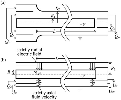
A schematic of a typical cylindrical DMA (Knutson and Whitby 1975) is shown in Figure 1a. Aerosol enters the instrument in flow at the left of the schematic along with clean particle-free sheath flow in . The two flows merge smoothly at the entrance to the annular classification region between inner radius and outer radius and proceed axially through the annulus. A radial electric field produced by a potential applied to the center rod draws particles of the opposite polarity charge inward across the sheath flow, with smaller, more mobile particles moving more quickly. At a distance downstream of the aerosol entrance slit, sample flow is extracted through a slit in the inner rod bringing with it particles of a narrow range of electric mobility. The remainder of the flow exits the end of the annular region as and is discarded. Under the most common operating conditions, the classified particle mobility is selected by varying the voltage, the flows are steady and balanced (, ) and the aerosol flow is on the order of one tenth of the sheath flow. A radial DMA (Zhang et al. 1995) in which the flow is directed radially between parallel disk electrodes operates under the same principal.

Figure 1. Schematics of (a) real cylindrical DMA and (b) idealized DMA with simplified flow and electric fields.

The DMA transfer function, designated as , is determined by analysis of particle motion through the classification region of the DMA. The classification region is loosely defined as the annular space between the two aerosol slits in the cylindrical DMA. More precisely, it includes the entire region in which the particles are subjected to the electric field, but excluding the typical transition back to ground potential occurring somewhere along the path of the exiting sample flow. Thus, the regions of protrusion of the field into the finite gaps of the aerosol slits beyond the annular bounds (, ) are included in the analysis. As the analysis typically does not include the bulk of the aerosol entrance and exit plumbing, particle losses in these sections due to diffusion or electrophoretic effects are not considered as a part of as defined here, though they are certainly pertinent to the overall transfer efficiency of the DMA.

There are three characteristics of the transfer function window of primary importance in the various applications of the DMA. When sampling a relatively broad distribution, the area of the window, along with the input distribution, determines the total concentration of transmitted aerosol. The centroid or mean mobility of the window determines the characteristic size of the transmitted particles. For many applications this is all that is required. But for other more demanding applications, the width of the window is also important as it determines the degree of dispersion of the exiting aerosol.

Flagan (1999) provided a thorough review of the development of electrical mobility measurement methods going as far back as a century. However, the beginning of the growth in significance within the aerosol community of the DMA hinged largely on the seminal work of Knutson and Whitby (1975) and subsequent commercialization of their prototype cylindrical DMA. In that work, they provide a rigorous derivation of the DMA transfer function for nondiffusing particles.

With increasing application of the DMA to smaller particles, the deleterious effects of particle diffusion on the transfer function soon became apparent. Particle diffusion can affect any of the three primary characteristics of (area, mean mobility, width), but its most pronounced effect is to broaden the transfer function. Building on the Knutson–Whitby analysis, Stolzenburg (1988) produced an approximate analytical model of the effect of particle diffusion within the classification region of the DMA. His model has been applied in a number of studies to characterize the performance of a DMA (Stolzenburg 1988; Zhang and Flagan 1996; Jiang et al. 2011; Cai et al. 2017; Stolzenburg et al. 2018) as well as to the recently developed ROMIAC (Mui et al. 2017). With the addition of empirically-determined adjustment factors for each of the above three key characteristics, these efforts have been significantly successful.

Here, the theory of Knutson and Whitby (1975) is briefly reviewed followed by a more extensive review of the Stolzenburg diffusion model. In each case, particular attention is focused on the assumptions (indicated by bullets •), approximations (indicated by diamonds ♦) and potential weaknesses of each analysis. Where available, suggested methods to improve on the approximations are given, though often these are numerical in nature applying only to the specific conditions of the calculations. In addition, efforts to fit analytical forms to measured transfer functions of real DMAs are briefly reviewed and compared, with recommendations for the most physically meaningful forms noted.

2. DMA transfer theory

The analysis of Knutson and Whitby (1975) for nondiffusing particles as well as that of Stolzenburg (1988) for diffusing particles may be broken down into two parts. The first part involves tracking an individual particle of a given electrical mobility, , from a streamline in the entering aerosol flow, , to a streamline in the exiting aerosol flow, . For the nondiffusing theory, there is a one-to-one correspondence while for the diffusing theory there is a probability distribution about the exiting streamline. In the second part of the analysis, the result of the first part is integrated over all combinations of entering and exiting aerosol flow streamlines. This integration step is essentially the same for the two analyses. Each of these parts is treated separately below.

2.1. Nondiffusing individual particle tracking

The theory of Knutson and Whitby (1975) for the transmission of nondiffusing particles through a cylindrical DMA assumes:

• axial symmetry of geometry, flows and electric field in the classification region

• incompressible laminar flow

• negligible space and image charges

• negligible particle inertial effects

• negligible particle diffusion effects.

These assumptions allow the definition of the conventional streamfunction, , and an analogously defined electric flux function, , such that (1) where and are radial and axial components of the flow velocity and and are components of the electric field. Using these two parameters as a new coordinate system to track particle motion in the plane, they demonstrated that the quantity , later termed the “particle streamfunction” () by Stolzenburg (1988), is a constant along the trajectory of a nondiffusing particle of mobility . Alternatively, this can be expressed as (2)

In particular, this is true for the change in going from the aerosol entrance slit () to the aerosol exit slit ().

If are the bounding streamlines of the entering aerosol flow, , and are the bounding streamlines of the exiting aerosol flow, , then and . From the definition of the streamfunction (Knutson and Whitby 1975), the bounding streamlines are related according to (3) where and are the entering sheath and exiting excess flows. Given prescribed flows, the change in streamfunction, , is readily calculated for any given pair of entering, , and exiting, , streamlines of the aerosol flows. In addition, Knutson and Whitby argued that the electric field must eventually disappear deep inside the DMA aerosol entrance and exit slits. This means that all particles that successfully traverse the DMA begin and end at the same values, and , of the electric flux function and is the same for all. The relationship between entering and exiting streamlines can then be stated as (4)

For use in the second part of the analysis, this can be written in terms of an equivalent probability distribution as (5) where is the Dirac delta function. For a particle entering at the aerosol inlet on is the probability of transfer to the range at at the aerosol outlet.

The mid-streamlines and streamfunction half widths of the aerosol flows are given by (6)

The centroid mobility of the range of successively transmitted particles is determined by finding the mobility of particle that enters on the mid-streamline, , of the aerosol inlet flow and exits on the mid-streamline, , of the aerosol outlet flow. The change in streamfunction for such a particle is given as (7)

Substituting and into Equation (2)(2) yields the centroid particle mobility as (8)

The final step of this part is to evaluate . Up to this point, the analysis of Knutson and Whitby (1975) has been completely rigorous given the assumptions listed. However, to obtain an analytical formula for an approximation must be made. If the perturbations arising from the aerosol entrance and exit slits are neglected, then

• ♦approximate the electric field as strictly radial and axially uniform such that .

With this, the change in electric flux function can be approximated as (9) and the centroid mobility¹ as (10)

As employed by Zhang et al. (1995), all of the Knutson and Whitby analysis applies equally well to radial DMAs with a simple adjustment of the calculation.

For the large aspect ratio, , of the cylindrical Knutson-Whitby prototype DMA as well as the commercialized version of similar dimensions, the approximation represented by Equation (9)(9) is quite accurate. According to Knutson and Whitby (1975), the true value of is overestimated by roughly 0.1%. However, the desire to reduce diffusion effects for particles in the nanometer range has driven design aspect ratios much closer to unity (Rosell-Llompart et al. 1996). In these instruments, the accuracy of this approximation can be significantly degraded leading to sizing errors using Equation (10)(10) . More accurate values for and can be obtained either through empirical calibration or numerical modeling of the true electric field.

It should be noted that the penetration of the electric field into the aerosol entrance and exit slits does not necessarily lead to violation of the axial symmetry assumption or any other degradation of the Knutson–Whitby analysis other than the calculation of The basic equation of the analysis (Equation (2)(2) ) applies equally well within these aerosol slit penetration regions beyond the nominal classification region. The modeling of Chen and Pui (1997) revealed a recirculation zone near the 90° corner of the aerosol entrance channel of the TSI Model 3071 DMA that acted to push the entering aerosol stream toward the upstream edge of the slit. They argued that this would increase the effective classification length of the DMA, but evidently did not verify this in their numerical model. From the above theory it is seen that the length is only used as part of the approximation in calculating from the electric field and the electric field is unaffected by the recirculation zone. The analysis of Knutson and Whitby (1975) is completely independent of the details of the flow field as long as it remains axisymmetric and laminar, including as it applies within the aerosol slits.

2.2. Diffusing individual particle tracking

In the analysis of Stolzenburg (1988) for the transmission of diffusing particles through a cylindrical DMA, all the assumptions of the Knutson–Whitby analysis are retained except the last. In its place, it is assumed

• particle diffusive displacements are small compared to the electrode gap.

This single additional assumption to a significant extent enables the approximations used in the diffusing particle tracking model.

To retain some of the elegance of the Knutson–Whitby analysis, Stolzenburg (1988) uses the particle streamfunction, , as the key coordinate for tracking a particle in his DMA diffusing transfer model. Since the value of and whether or not it lies within the bounds of the aerosol exit flow determine the success or failure of transmission for a particle, the objective is to deduce the probability distribution of for a diffusing particle entering the DMA at a given This is equivalent to finding the probability distribution of for a particle entering the DMA on , the beginning nondiffusing particle streamline.

Letting represent distance along this nondiffusing particle streamline (constant ) and x the distance perpendicular to the particle streamline (in the direction of ), then and an azimuthal coordinate form an orthogonal curvilinear coordinate system localized about the particle streamline. Due to the axial symmetry, diffusion in the azimuthal direction is of no consequence. Also, for constant voltage operation of the DMA, diffusion in the direction along the particle streamline has no direct effect on particle sizing, though it may affect arrival time at the downstream detector. (For continuous scanning operation of the DMA, diffusion in this dimension can have important consequences.) For constant voltage operation, only diffusion in the cross-stream direction affects particle sizing and transmission probability. In this way, the diffusion model may be pictured as an expanding one-dimensional bell-shaped probability distribution orthogonal to the nondiffusing particle streamline and translating along it as the particle traverses the classifier.

The analysis of diffusion in this single dimension begins with the Einstein equation for diffusive displacement, , where is the mean square diffusive displacement from the location at time of a particle of diffusivity . Since diffusion is based on actual physical distance, to relate this to particle streamfunction, a relationship must be found between and The gradient of is in the same direction as , and from the definitions of streamfunction and electric flux function (Knutson and Whitby 1975), Stolzenburg showed that where is radial position and is the magnitude of particle velocity.

To allow transformation of this differential relationship into a linear finite form for small diffusive displacements, Stolzenburg makes the following approximations:

• ♦neglect cross-stream shear

• ♦neglect the skewing effect of radial acceleration in the converging electric field.²

In addition, to further simplify the diffusion analysis:

• ♦neglect effects of streamwise diffusion on the cross-stream probability distribution

• ♦neglect diffusion losses to walls in the classification region of the DMA.³

Using Monte-Carlo simulations of diffusing particles in a cylindrical DMA similar to the TSI 3071, Hagwood, Sivathanu, and Mulholland (1999) have shown that axial diffusion (essentially the same as particle streamwise diffusion for this large aspect ratio DMA) has negligible effect even for very large diffusive particle displacements. For a fully developed flow profile, the simulations also show negligible particles losses to walls down to 3 nm at a sheath flow of 10 L/min. For a 1:10 aerosol to sheath flow ratio (), this corresponds to a diffusive broadening (, defined below) of the transfer function to more than five times its nondiffusing width. Though losses are more pronounced for plug flow, this indicates that the last two approximations are justifiable within the assumption of small diffusive displacements.

For the previous two approximations, both cross-stream shear and radial acceleration add nonlinearity to the relationship leading to skewing of the particle cross-stream probability distribution. The former has no direct effect on the overall spread of the probability distribution while that of the latter is accounted for by the linear part of the relationship. Cross-stream shear in a developed fluid flow profile reverses direction as the particle passes the radius of maximum flow velocity. This means the skewing effect of the later segment of the particle trajectory will tend to offset that of the earlier part. However, the skewing effect of radial acceleration is all to one side. The simulations of Hagwood, Sivathanu, and Mulholland (1999) show skewing of the peak of the transfer function toward higher voltages (lower mobilities) on the order of 1% at 10 nm at which size diffusion has broadened the transfer function (, ) by a factor of 1.8. This corresponds to diffusive particle displacements on the order of the width of the nondiffusing aerosol stream through the DMA at so again these approximations are justifiable within the assumption of small diffusive displacements.

With these approximations, the problem is now similar to one-dimensional diffusion in a quiescent or uniformly translating medium,⁴ which yields a Gaussian probability distribution centered on the beginning nondiffusing particle streamline. Using the approximation of a local linearization of on about , the Einstein relationship can be transformed to particle stream function space as (11) where is the standard deviation of the probability distribution in the coordinate.

To obtain the total spread, , in the probability distribution when the particle reaches the vicinity of the aerosol exit slit, the foregoing differential equation must be integrated over the path of the nondiffusing particle. Though one could evaluate this integral for each unique trajectory of a successfully traversing nondiffusing particle, this would add a great deal of complexity to the final result that is already compromised by these numerous approximations. It is anticipated that the variation in calculated from the integral along these different trajectories would be relatively small for a typically narrow nondiffusing transfer function. The approximation is made to

• ♦neglect variation in over the range of nondiffusing particle trajectories.

Thus, the integral is only evaluated for a single characteristic trajectory designated as , which represents the path of a nondiffusing particle of mobility that enters the classification region on streamline and exits on streamline . The integral is then expressed as (12)

The foregoing approximations lead to a Gaussian probability distribution for of standard deviation centered on the nondiffusing particle streamline, , determined by the fluid streamline, , on which the particle entered the classification region. This is expressed as (13)

Equation (13)(13) is the diffusing particle equivalent of the transfer probability function given in Equation (5)(5) for nondiffusing particles.

2.3. Evaluation of the diffusion parameter

What remains of this part is to evaluate as represented by the integral of Equation (12)(12) . To do this will require details of both the fluid velocity and electric fields. To obtain an analytical expression it is necessary to make some significant simplifications to both fields specific to the DMA configuration (e.g., cylindrical vs. radial). But before this, it is useful to begin a dimensional analysis of Equation (12)(12) . The first step of this is to find appropriate scaling factors for the various physical parameters.

is representative of the total classification potential of the DMA while , as the diffusional spread in , represents a degradation in that potential. Scaling the latter by the former and noting the relationship between particle diffusivity and electrical mobility (14) the DMA diffusion parameter (Equation (12)(12) ) can be rewritten as (15)

In the rightmost expression of Equation (15)(15) , each of the three groupings of parameters (the last including the integral) is dimensionless. The inverse of the first grouping has been shown by Flagan (1999) to correspond to a classical definition of the Peclét number as a ratio of the flux due to directed motion to that due to diffusion in which the directed motion of the particle is its electrophoretic migration. As such, he labeled it the migration Peclét number defined as⁵ (16)

Aside from his derivation, in this form it is perhaps more readily recognized as a ratio of the energy of directed motion to that of diffusion. Regardless of interpretation, it represents the relative importance of the directed migration (classifying action) compared to particle diffusion (randomizing action).

The second grouping of parameters on the right side of Equation (15)(15) is readily interpreted as a dimensionless particle electrical mobility defined as (17)

This parameter reflects the fact that in this approximation, though the particle is constrained to follow the path of a nondiffusing particle of mobility characteristic of the DMA operating parameters, the true particle diffusivity corresponding to is used to calculate the rate of broadening of the probability distribution about that path.

Equation (15)(15) can now be rewritten as (18) where (19)

depends only on the operating parameters of the DMA. Additionally, it will be shown that it is fundamentally of order one such that this parameter is independent of the scaling of the DMA or its absolute flows or analyzer voltage. Thus, the main dependence of the diffusion parameter, , is all encompassed within the migration Peclét number, .

is dependent on particle size through the dimensionless electrical mobility, . Let be the diffusion parameter evaluated at the centroid mobility of the DMA transfer function such that (20)

Then represents a characteristic magnitude of the diffusional broadening of the transfer function, independent of particle mobility diameter but not particle charge.

Up to this point, the analysis applies to any axially symmetric configuration of the DMA. To complete the dimensional analysis of , configuration-specific scaling factors are needed for the physical parameters within the integral. At least for the original relatively high-aspect-ratio cylindrical DMAs, the fluid flow is the dominant contribution to particle velocity, , so the average axial fluid velocity, , can be used to scale . is used to scale radial position, , while an estimate of transit time, ̂t, provides an appropriate scaling for time, , in the integral. The transit time for the DMA classification region can be estimated from the radial particle velocity derived from the Knutson–Whitby approximated electric field,⁶ , and the particle mobility, , as (21)

This can be integrated to get (22)

As the particle accelerates moving inward toward the axis, the time to reach (hypothetically according to Equation (22)(22) ) is not that much greater than to reach for typical DMA annular aspect ratios. Thus, the scaling time is taken as (23)

Using the indicated scaling factors, the following nondimensional physical parameters are defined: (24)

In addition, the dimensionless geometry scaling ratios (25) are defined along with the flow ratios (26)

With these definitions, becomes

Noting that

can be rewritten as (27)

Thus, in this approximation depends on the ratios of dimensions or flows and on the shape of the assumed flow profile, but not on the absolute values of any of these.

To analytically evaluate the integral in Equation (27)(27) , it is now necessary to introduce the previously mentioned simplifying approximations to the electric and fluid velocity fields. For the former, the same approximation is used as that of Knutson and Whitby (1975) to evaluate —that is, to ignore the effects of the aerosol entrance and exit slits on the electric field. For this calculation it is also necessary to ignore the effects of the slits on the fluid velocity field as well as any axial variation in the velocity profile. Thus,

• ♦approximate the fluid velocity field as strictly axial and axially uniform such that , .

The nearly equivalent DMA configuration is illustrated in Figure 1b.⁷ Of all the approximations made in the diffusion analysis, this last has perhaps the greatest potential impact on the accuracy of the model. A more thorough discussion of this follows the remaining development of the evaluation.

With these approximations it is possible to separate the and components in the integral of Equation (27)(27) and to evaluate it in analytical form. The radial motion of the particle is independent of the flow field and axial position and can be solved outright as in Equation (22)(22) . Using the preceding definitions of nondimensional parameters, this can be written in dimensionless form as (28)

Substituting this into the integral, the limits of integration are now determined by the radial locations, and , of the mid-streamlines, and , of the respective aerosol inlet and outlet flows in the simplified fluid flow field of the model (Figure 1b).

Let (29) be the dimensionless flow velocity profile, , and cumulative flow fraction, , between radial position () and the outer wall of the annular classification region at (). Then the positions of and are determined through iterative solution of (30)

Noting that the integral of Equation (27)(27) can be separated into (flow) and (migration) contributions to . For the former, (31) where (32)

Using Equations (21)(21) , (10)(10) , (25)(25) , and (26)(26) , the components of the integrand of the contribution can be rearranged to and the contribution itself becomes (33)

Combining the and contributions finally yields for the cylindrical DMA (34)

The formulations of , , and for both fully developed and plug flow within an annulus are set forth in the summary of equations for applications in the Appendix.

With a slight rearrangement of factors in Equations (16)(16) , (18)(18) , and (34)(34) , these match the formulation of the diffusion parameter for cylindrical DMAs given in Flagan (1999). This also agrees with the later summary of Stolzenburg and McMurry (2008), though the equation for contained an error and the formula for was omitted in the Appendix. Though all three of these formulations give the same computational results, note that and as defined here are different from both those in Stolzenburg and McMurry (2008) and also those in Flagan (1999).

It is important to note that the original formulation in Stolzenburg (1988) differs from all of these and produces different computational results. The formulation in the main text there is equivalent to setting and in Equation (34)(34) . That is, the integral defining the diffusion parameter was integrated from the wall at to the wall at while still using the simplified fields as in Figure 1b. This difference is explained in greater detail in the online supplemental information (SI). Within the limits of the approximated fields, this results in an overestimation of of roughly 3–7% for a range of cylindrical DMAs operated with flow ratio near .

The discussion in the SI also serves to highlight the effect of neglecting the radial flow component in the vicinities of the aerosol entrance and exit slits of the real DMA (Figure 1a). The neglect of radial flow in the approximation of given here results in a slight underestimation of the magnitude of the diffusion parameter. With higher flow ratios, , the radial flow will be stronger leading to a greater discrepancy. Cylindrical DMAs with shorter aspect ratios are more sensitive to the effects of the slits leading to a greater discrepancy for these as well. Though the original formulation of in Stolzenburg (1988) provides a higher estimate, that analysis does not arrive at this in a way that reflects the true contribution of the radial flow. Thus, the difference between these two estimates cannot be considered to be indicative of the error due to neglect of radial flow. There is also the error due to the assumption of the flow profile and its constraint of constancy as the flow moves down the annulus. The true flow field is undoubtedly much more complex resulting in a largely unknown degree of variation in the true value of as compared to the approximation represented by Equation (34)(34) . The resolution of these uncertainties will require the numerical modeling of the true flow field and electric field using the accurate geometry of the real DMA combined with numerical calculation of from Equation (19)(19) .

2.4. Integration of particle tracking results

In the second part of the transfer analysis, the result of the individual particle tracking is integrated over all combinations of entering and exiting aerosol flow streamlines. This integration step is essentially the same for the two analyses.

From the individual particle tracking, (Equation (5)(5) or (13)) is the probability of a particle that enters the classification region on streamline successfully transiting the region to exiting streamline . The integrated transfer probability will also depend on the probability of an entering particle arriving at the aerosol entrance slit on streamline . Together these are combined to give the integrated probability as (35)

The Knutson and Whitby (1975) theory assumes a

• uniform inlet probability distribution (nondiffusing model)

that can be expressed as (36)

As the simplest approximation, the Stolzenburg (1988) diffusing particle transfer model retains this to

• ♦approximate the inlet probability distribution as uniform (diffusing model).

Since is a constant, it can come out of the outer integral of Equation (35)(35) leaving a double integration of alone.

For the nondiffusing case, the inner integration of the Dirac delta function, , of Equation (5)(5) in Equation (35)(35) yields the sign function, , and the double integration yields the absolute value function, . For the diffusing case and the normal distribution, , of Equation (13)(13) , the first integration results in the error function while the second results in (37)

In either case, the result of the double integration is four terms, each of which corresponds to one of the four possible combinations of evaluated at the bounding streamfunction values of and . Noting that each such difference can be expressed in terms of flows (Equation (3)(3) ) in two ways via the flow balance relationship, , a degree of symmetry in the final nondimensionalized results can be obtained by averaging these two expressions. An example of this type of transformation is (38)

The nondiffusing form, , of the transfer function is nonzero over the finite range thereby limiting the range over which the individual terms need be evaluated. However, the diffusing form, , of the transfer function is physically meaningful and mathematically nonzero over the entire range while its individual terms go to infinity at either end of that range. Even with the integral restricted to the positive range of the spectrum, to avoid small differences of large numbers it is best for computational purposes to evaluate in the equivalent form (39) where the diffusion correction is found from by replacing with given by (40)

Note that . Putting all this together, the final dimensionless integrated forms of Equation (35)(35) are given in the Appendix.

The summary of equations for applications in the Appendix provides a compilation of the equations for calculating theoretical transfer functions for both cylindrical and radial DMAs for either fully developed or plug flow. Though some factors in the calculation of the diffusion parameter, , are grouped differently, these equations yield the same results as in both Flagan (1999) and Stolzenburg and McMurry (2008). The Appendix indicates the relationship between the different definitions of the parameter in these publications. Using these equations, the Appendix includes a comparison of the diffusion effects in a number of different DMAs.

2.5. Inlet probability distribution alternatives

Returning to Equation (36)(36) , the assumption of a uniform inlet probability profile for the nondiffusing particle model should be quite accurate. With no diffusion losses in the DMA aerosol entrance plumbing, there is little else to perturb the uniformity of the concentration profile. This is not the case, however, for the diffusing particle model such that this represents a significant approximation. In reality, diffusion losses to the walls of the aerosol entrance channel leading up to the entrance into the classification region reduce concentrations (and probabilities) near the edges of the entrance slit leading to a notably nonuniform inlet probability profile and altered integrated transfer probability. Similarly, the transfer through the classification region affects the concentration profile at the beginning of the DMA aerosol exit plumbing and the integrated transport efficiency through that section. In general, within any plumbing section with continuous laminar streaming flow, the integrated aerosol transfer efficiency through any subsection will depend on what happens upstream.

To deal with the linkages between the losses in and transfer through these different sub-sections of the DMA, one could numerically model the entire DMA as a whole as was done for the ROMIAC in Mui et al. (2017). However, the time and resources required for such an extensive analysis are not always practical. Technically, the continuous laminar flow region can easily extend beyond the nominal limits of the DMA, making such an analysis dependent on losses within the upstream plumbing as well. So for practical reasons, it may be necessary to neglect some of these dependencies or use mixing orifices to break the linkage though at the cost of increasing the losses.

An alternative approach is to extend the analytic model of Stolzenburg (1988) to account for the effects of losses within the DMA aerosol entrance and exit plumbing. Following Stolzenburg (1988, Appendix E) and assuming a uniform concentration at the entrance to the DMA, let be the probability of a particle transiting the DMA entrance plumbing to a streamline in at at the entrance to the classification region and be the total probability of successfully transiting the entrance plumbing. Then the inlet probability profile for the classification region is just (41)

Similarly, for a particle starting on streamline at the exit of the classification region, let be the probability of successfully transiting the DMA exit plumbing and be the average probability of transiting the exit plumbing. Then the linkage of the exit plumbing losses to the classification region can be accounted for through use of (42) in the integrated transfer function as (43) and the penetration through the DMA as a whole is given by Since losses are dependent on particle size, the shapes of both and are size-dependent. As many DMA designs break up the streaming flow shortly downstream of the aerosol exit slit of the classification region, attention is focused in the following on accounting for a nonuniform inlet probability profile, while maintaining the approximation (Equation (35)(35) ).

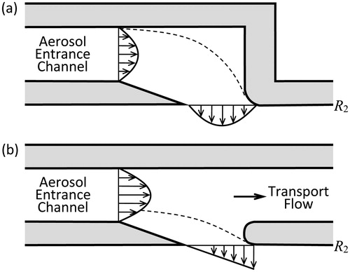
A typical cylindrical DMA aerosol entrance channel is illustrated in Figure 2. For an entrance channel with no augmentation of the aerosol inlet flow (Figure 2a) the losses may be relatively symmetric leading to a somewhat parabolic shaped inlet probability profile. For a laminar flow inlet with extra transport flow on one side of (Figure 2b) such as in the TSI nano-DMA (Chen et al. 1998), the losses within may be extremely asymmetric leading to a nearly linear ramp-like profile from zero at the edge of the entrance slit corresponding to the wall of the entrance channel to a maximum at the other edge having just separated from the transport flow. In either case, the fluid velocity would have a profile similar in shape to that of the corresponding concentration profile.

Figure 2. Schematics of the approximate flow and concentration profiles for a highly diffusive aerosol in the aerosol entrance channel and at the entrance slit (a) without transport flow and (b) with transport flow.

As depicted in Figure 2, the linear or parabolic profiles of the radial fluid velocity component, and aerosol concentration, , at the aerosol entrance slit at represent approximate limiting cases of perturbations of the inlet probability distribution. The parabolic profiles of Figure 2a can be represented as (44) and the linear profiles of Figure 2b as (45) where is the half-width of the aerosol entrance slit and is at the physical midpoint of the slit.

These simplified concentration profiles are analytically tractable but the parabolic profile is only a rough approximation to the true fully-developed concentration profile of the aerosol entrance channel with no transport flow. A possibly more accurate representation of this limiting case is to model the entrance channel as Poiseuille (parabolic) flow between parallel plates with a fully-developed concentration profile at the aerosol entrance slit. For this parallel plate approximation (similar to the Graetz solution for round tubes), the numerically computed first order eigenfunction provides the dimensionless concentration profile .

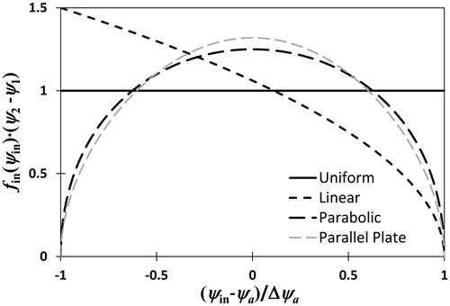
To model a nonuniform inlet probability distribution such as these, can be obtained from the radial flow velocity, , and aerosol concentration, , at the aerosol entrance slit as (46) where and is the average entering aerosol concentration. Using Equation (46)(46) , the distributions corresponding to uniform, linear, parabolic and parallel plate inlet profiles are shown in Figure 3.

Figure 3. Inlet probability profiles for limiting cases of diffusion losses in the aerosol entrance channel—“uniform” (no losses), “linear” (transport flow with asymmetric losses), “parabolic” (no transport flow with symmetric losses), “parallel plate” (numerical approximation to no transport flow with symmetric losses).

Substituting Equation (46)(46) into Equation (43)(43) or (35) yields the modified transfer function, though finding an analytical form may be difficult. If can be approximated by a polynomial⁸ in , then it is still possible to obtain an analytic expression for The results of this are given in detail in the SI. A closed but somewhat more complex form is found, and transfer functions are plotted for polynomial fits to the inlet probability profiles shown in Figure 3. However, a finite-term polynomial approximation can lead to unrealistic oscillations in the long, low-probability tails of , which may not be acceptable in some applications.

Stolzenburg (1988, Appendix E) sought an approach that would essentially retain the original formulation of but with modified parameters. He reasoned that a significant degree of diffusional broadening of the transfer function would tend to obscure the details of the altered inlet probability distribution, only retaining information on the mean and standard deviation of that distribution. Using that idea, Stolzenburg proposed to reduce the width of the uniform input distribution to where and and are chosen to match the mean and standard deviation of the real inlet probability distribution. The new limits are substituted for and in Equations (35)(35) and (36)(36) and the integration proceeds as before. The analysis continues by defining modified values of , , and even that can then be used in the original formulations for and .

The full development of this model can be abbreviated here to obtain an estimate of the possible magnitude of effect of a perturbed inlet probability profile on the mean and standard deviation of the transfer function. The primary effects are to the nondiffusing contribution to these parameters of the transfer function, though there can be a small adjustment to the diffusion parameter as well.

From Stolzenburg and McMurry (2008), let and represent the mean and variance of the transfer function given by (47)

The first term on the right side of each equation represents the nondiffusing contribution to the parameter. The relationship of these nondiffusing terms to and can be determined through calculation of moments of the nondiffusing transfer function using Equation (43)(43) for and interchanging the order of integration. It is found that (48) where and are the mean and standard deviation of and and are the corresponding quantities for . For uniform and , , , , and Equation (48)(48) yields the nondiffusing terms of Equation (47)(47) . From this it follows that changes to the mean and variance of the transfer function caused by the perturbation of the inlet probability distribution only are given by (49)

So the question becomes how much are and perturbed by the nonuniform inlet probability distribution.

The moments, mean, and variance of each profile are calculated as (50)

The results of these calculations for both the uniform and nonuniform profiles are shown in Table 1 where the mean is scaled by and the variance by .

Table 1. Inlet probability distribution, , parameters and their effect on the transfer function.

Parameter	Uniform	Linear	Parabolic	Parallel plate
	0	−1/5	0	0
	1/3	48/175	59/231	0.24052
	0	0.01	0	0
	0	−0.00015	−0.00019	−0.00023

In Equation (49)(49) , the changes in the parameters of are scaled by rather than . To relate the preceding results for the parameters of to changes in the mean and variance of the transfer function, Equation (49)(49) , the flow ratio is needed. The values of the change parameters of Equation (49)(49) are given in Table 1 for a cylindrical DMA operated with balanced flows, , and a flow ratio of . As these results are for limiting cases of a nonuniform inlet probability distribution, it is seen that the maximum offset in the mean of the transfer function is just 1%. However, for the same DMA operated as indicated, the nondiffusing contribution to the variance of the transfer function is given by such that the changes represent as much as a 14% reduction in the nondiffusing portion of the variance.

As noted earlier, the diffusion parameter, , can also be affected by a nonuniform inlet probability distribution. Recalling that was calculated as an integral along the characteristic trajectory of a nondiffusing particle of centroid (mean) mobility , this path can be adjusted according to the offset in the mean of the transfer function. However, as noted above, this offset is at most 1% and is well within the variation of possible nondiffusing trajectories already neglected in the calculation of . For small to moderate diffusional broadening (compared to the nondiffusing contribution) of the transfer function, this effect will be small compared to the change in the nondiffusing portion of the variance.

3. Fitting theory to measured DMA transfer functions

In practice, the performance of real DMAs often differs from the predictions of theory for various reasons. In many cases, it is suspected that the flows in the DMA violate the laminar or axial symmetry assumption. This may be due to a design or machining flaw, operation beyond design parameters, aerosol loading, or unknown factors. Alternatively, a discrepancy between measurement and theory may indicate a limitation of the theory. For instance, for very short aspect ratio DMAs, the approximation that led to Equation (9)(9) for loses accuracy leading to errors in the predicted centroid mobility. In either case, it is important to verify the performance of a DMA experimentally.

The accepted way to do this is to challenge the DMA with a monodisperse, or near monodisperse, aerosol of known mobility distribution and to measure the concentration both upstream and downstream of the DMA as its mobility window is scanned across the input mobility range. The DMA voltage scan may be step-wise or effectively continuous, though slow enough to avoid significant distortions of the transfer function. Until fairly recently, the best source of aerosol for such an experiment was from another DMA with a broad distribution as input. The resulting configuration is commonly referred to as a tandem DMA, or TDMA, experiment. More recently and as DMAs were developed for and tested in the nanometer size range, truly monomobile aerosols have been available through the electrospray of solutions of large-molecule salts (Ude and Fernández de la Mora 2005). These large ion aerosols can be used directly to challenge the test DMA or pre-classified with another DMA to isolate a single monomobile ion species.

If denotes the mobility distribution of the challenge aerosol, then the DMA output concentration as a function of classifier voltage can be calculated as⁹ (51)

With the finite dispersion of as produced by the upstream DMA in a TDMA experiment, it is clear that the measured response of the system does not immediately yield the DMA transfer function Even for a monomobile () challenge aerosol for which is represented by a Dirac delta function as , the response, (52) of the system is not in the standard form with voltage fixed. In either case, some level of inversion of the data is required to obtain the measured transfer function.

As noted by Stratmann et al. (1997), the best way to invert Equation (51)(51) in the presence of measurement noise is to use a parameterized version of the measured transfer function with parameters determined by the best fit of predicted responses (Equation (51)(51) ) to measured responses. The form, , of the transfer function used in this fitting procedure is obtained from the theoretical transfer function, or , with additional adjustable parameters. It is usually sufficient to add three adjustable parameters: one for the area of the transfer function, one for the mean or centroid, and one for the width. Choosing fit parameters in this way means that they are nearly completely independent of each other. Thus, adjusting the area fit parameter does not affect the mean or width and the same for all other combinations. The independence is not complete in a few cases but the interaction between the parameters is usually quite low.

The area adjustment can be modeled as an efficiency factor, , multiplying the transfer function. This accounts for any diffusive particle losses to walls or electrophoretic losses in the high voltage transition of the aerosol exit plumbing. The diffusing particle model of transfer through the DMA classification region neglects any particle losses to walls there and, as was noted, the work of Hagwood, Sivathanu, and Mulholland (1999) verified this to be a good approximation even for fairly large diffusive displacements.¹⁰ Thus, the efficiency factor is primarily a measure of penetration through the aerosol entrance and exit plumbing. As such, it is not really a part of which only characterizes the classification region as defined here.

These plumbing losses are often adequately modeled by a diffusivity- or size-dependent penetration efficiency factor, , and treated as independent of . However, as was discussed with regard to the classification region inlet probability profile, there is a degree of dependence between losses within any subsection of the DMA and other upstream subsections. This may be handled via the techniques described above or by numerically modeling the whole DMA as one (e.g., Mui et al. 2017). Though the latter approach may be more accurate, it is computationally intensive and would need to be completely redone for any change in the instrument plumbing.

For very large diffusive displacements of particles transiting the classification region, diffusive losses to the walls of the classification region can become significant even for particles of mobility near the centroid of the transfer function. Such losses depend on both particle diffusivity and electrical mobility, changing the shape and reducing the area of the transfer function. The diffusing transfer theory of Stolzenburg (1988) was never intended to encompass such large diffusive displacements. In such a scenario, the aerosol transport might best be solved via Monte Carlo simulations (e.g., Hagwood, Sivathanu, and Mulholland 1999) or the particles modeled as a dilute (charged) gas component with transport solved via the convective diffusion equation (e.g., Mui et al. 2017).

Flow measurement errors and the approximation in calculating can lead to error in the calculated centroid mobility, and discrepancies between measured and predicted particle mobilities and sizes. This can be accommodated in fitting the theoretical model to measurements with the inclusion of an adjustable multiplier, (or ), of . may be readily interpreted as an adjustment to the DMA size calibration via , dependent on and . The latter depends on and the effective (cylindrical DMA) or (radial DMA). Any of these base dimensional parameters could be in error.¹¹ may also represent an error in particle mobility, , generally treated as known as from a reference DMA or a monomobile ion. For transfer function measurements, is often found to be within 2–3% of unity and is not included in some applications of this fitting algorithm.

Most of the common, correctable nonidealities—e.g., flow mixing or asymmetry—of real DMAs directly reduce the resolution of the transfer function by increasing its width. For , the width is determined by (and to a significantly lesser extent by ) and a multiplicative adjustment, , to that can be used to fit the width of the measured transfer function. For , also contributes to the width and the width adjustment is typically applied to that. Both approaches have been used in past work as indicated below.

As noted earlier, the area, centroid and width adjustments should be largely independent of each other. However, a significant adjustment may imply an error in a base parameter affecting or and subsequently or or even . Thus, for accurate values of any of these adjustment parameters, it is important to determine the source of the discrepancy. If the base parameter in error can be identified, then all derived parameters (e.g., , , , ) should be corrected accordingly. Ideally, this would be done prior to fitting the data. However, post-fit corrections to the adjustment parameters can be applied based on maintaining the same fitted width or transmitted particle concentration. Thus, , , and can be corrected according to (53)

Note that and are sensitive to flow errors while is affected by nearly any error in base parameters.

In the inversion of Equation (51)(51) , the best fit of predicted to measured responses is usually determined by the minimization of an error parameter. This generally takes the form of the sum of squares of residuals (SSR), or remaining differences between predicted and measured responses. The residuals may be individually weighted to adjust their relative importance in the fit. A common weighting is to divide each residual by the estimated uncertainty in the corresponding measurement. The statistical probability distribution for such a weighted SSR is given (usually only approximately) by the function, the sum of squares of unit normal probability distributions. In addition, to reduce the effects of temporal variations in the source aerosol concentration, measurements downstream of the DMA being tested can be normalized by simultaneous measurements upstream of the DMA.

The SSR minimization is accomplished through a search approach, requiring integration of all of the predicted responses (Equation (51)(51) ) for each trial in the multidimensional adjustable parameter space. If the trial integrations must be done numerically, this can be very computationally intensive. Fortunately, this is only required in the case of a TDMA experiment using based on . For a TDMA experiment using , or based on , for each DMA, the integrand in Equation (51)(51) is piecewise quadratic in and can be readily integrated analytically. As indicated earlier, for monomobile challenge aerosols the integrals can be eliminated entirely, though a search is still required.

In the data inversion for a TDMA experiment to measure the transfer function, there is the inherent question as to which DMA the adjustments should be made. The application of adjustments to the transfer function of the upstream DMA (DMA1), the downstream DMA (DMA2), or equally to both DMAs all yield comparable fits to the data. So other criteria beyond the single TDMA experiment must be used to determine what is appropriate or an assumption must be made.

3.1. Previous transfer function measurements and inversion

Though the TDMA technique was introduced and applied in several prior studies, the first published report of a true data deconvolution algorithm as described here is that of Rader and McMurry (1986) in the measurement of droplet growth and evaporation. They used a 3-parameter fit based on the nondiffusing transfer function of Knutson and Whitby (1975) with the width adjustment (equivalent to ) applied to both DMAs. Their fit error parameter consisted of a summation with residuals divided by estimated measurement uncertainties. They did not explicitly report any results corresponding to the measurement of transfer functions.

Stolzenburg and McMurry (1988) (reference included in the SI) developed a similar algorithm, TDMAfit, for similar use but also recognized its utility in measuring the DMA transfer function. Five newly fabricated DMAs of similar design and dimension as the TSI 3071 were tested against this commercial DMA. Nominal flow rates of 1 and 10 L/min aerosol and sheath flows (, ) were used for both DMAs. Flows exiting DMA1 passed directly to corresponding flows in DMA2 to ensure identical total flows through both instruments.¹² The DMA1 voltage was set to 8 kV corresponding to a centroid mobility diameter of 0.278 µm thereby minimizing the effects of diffusion. Assuming the reference DMA (DMA2) to be operating according to theory, they fit adjustment factors , , and for the test DMA (DMA1) according to Table 2 as reproduced here from that work. They found that the fitted width of the transfer function was on average 5% greater than the predicted while nearly all measurements fell within +10% (). The DMA2 penetration efficiency averaged about 97% and the DMA2 measured mobility was about 0.9% lower than that of DMA1, corresponding to an apparent diameter growth of 0.7%. This discrepancy is within residual flow measurement uncertainties. Thus, both DMAs in the TDMA setup performed close to the ideal.

Table 2. Data from TDMAfit evaluations of five DMAs, from Table 4 of Stolzenburg and McMurry (1988).

Unit no.	fβ	fN	fV	GD
4	1.06 ± 0.02	0.98 ± 0.01	1.016 ± 0.001	1.011 ± 0.001
5	1.04 ± 0.04	0.98 ± 0.02	1.011 ± 0.001	1.008 ± 0.001
0	1.03 ± 0.03	0.95 ± 0.02	1.007 ± 0.001	1.005 ± 0.001
2	1.09 ± 0.04	0.96 ± 0.02	1.010 ± 0.002	1.007 ± 0.001
3	1.05 ± 0.04	0.95 ± 0.02	1.007 ± 0.001	1.005 ± 0.001
3	1.02 ± 0.06	0.97 ± 0.03	1.005 ± 0.002	1.004 ± 0.002
Low	1.02	0.95	1.005	1.004
High	1.09	0.98	1.016	1.011
Mean	1.05 ± 0.03	0.97 ± 0.02	1.009 ± 0.004	1.007 ± 0.003

is the apparent diameter growth factor.

Stratmann et al. (1997) developed an algorithm to deconvolute TDMA data fitting only area and width using an -based model and minimization of the SSR, presumably unweighted. The algorithm can achieve the fit adjusting the transfer function of only one DMA or of both assuming they are identical. In addition, using Gaussian as well as triangular transfer functions, they demonstrated that the TDMA technique of measuring transfer functions is relatively insensitivity to the shape of the transfer function, at least in terms of the recovered area. Thus, due to the simplicity of the calculations compared to the numerical integrations required using from the Stolzenburg model, they make an argument for continuing to use the model with size-dependent parameters to characterize the transfer function even in the presence of significant diffusional broadening.

Using this algorithm to characterize four different DMAs, Fissan et al. (1996) determined the transfer function of the first using the identical DMA mode. Transfer functions of the remainder were determined using the first DMA as a known reference and the other mode of the algorithm. The reference DMA showed significant nonideal broadening of the transfer function. Hummes et al. (1996) re-measured the transfer function of one of the nonreference DMAs from the previous study (TSI 3071 short DMA) using the identical DMA mode of the algorithm, finding it to perform close to near ideal predictions of the Knutson–Whitby model. Using the identical DMA mode, Birmili et al. (1997) measured the transfer function of five different pairs of nominally identical DMAs, finding all but one (TSI 3071 long DMA) to exhibit significant nonideal broadening of its transfer function.

Martinsson, Karlsson, and Frank (2001) demonstrated a method using the Stratmann et al. (1997) algorithm to unambiguously apportion nonideal DMA performance to individual DMAs. The procedure uses data from a series of three TDMA experiments with three different DMAs rotating through the DMA1 and DMA2 positions in turn, returning the fitted transfer functions for each of the three DMAs. Penetration efficiencies are found for DMA2 from individual TDMA experiments while width parameters for all three DMAs are found in one final grand fit to all the data. Using this technique, Karlsson and Martinsson (2003) demonstrated that nominally identical DMAs can exhibit distinctly different levels of nonideal broadening of the transfer function, thereby calling into question much of the foregoing DMA characterization effort. Assuming independence of diffusive and nonideal broadening effects and relying on the accuracy of the Stolzenburg model to estimate the former, they formulated a method by which the size dependence of a DMA transfer function can be estimated from a measurement of it at a single particle size. Though based to some extent on the Stolzenburg model, the method bypasses the significant computational burden of that to offer a readily utilized algorithm for practical applications.

All of the above TDMA measurements of DMA performance have used a fitted transfer function based on the nondiffusing transfer function of Knutson and Whitby (1975). As already noted, the same technique based on the diffusing transfer function of Stolzenburg (1988) is very computationally intensive with far fewer examples recorded. Stolzenburg (1988) used this method to test the diffusing transfer model on a pair of TSI 3071 long DMAs. He used a three parameter fit with to adjust the width of both transfer functions equally and a summation, or weighted SSR, based on a constant relative uncertainty and ratios of concentrations downstream and upstream of DMA2. Later, Zhang and Flagan (1996) used a similar procedure to characterize the Caltech radial DMA. They used the same adjustment factors and a based on Poisson statistical uncertainties. Both studies showed acceptable fits to the data and broadening of the transfer function consistent with combined diffusional and nonideal flow contributions. Also observed by both was an anomalous shift in the DMA2 response toward lower mobilities (higher voltages, ), increasing in magnitude as the diffusion effect increased. This shift was greater than could be readily explained by uncertainties in base parameters and a satisfactory explanation for it has proved elusive.

Seeking to eliminate the shape assumption from the fitting process, Li, Li, and Chen (2006) proposed a spline model of the transfer function with linear or higher order segments but otherwise fitting to TDMA data as in the other methods. Using a 12-segment linear spline, they demonstrated the capability of recovering from simulated TDMA data close approximations to diffusing and nondiffusing forms of the transfer function as well as to an artificially skewed form of the latter. The method was shown to be relatively insensitive to noise in the data as well. Both the spline and the diffusing transfer model were used to fit TDMA data from the nano-DMA (Chen et al. 1998) producing very similar results. Unfortunately, there was no information given regarding placement of node points for the spline. From the examples given, it appears that the method assumes the peak of the transfer function is known a priori such that a node point there can allow for the sharp slope discontinuity of nondiffusing and near nondiffusing transfer functions. It also appears that nodes were placed a priori at the other points of slope discontinuity of the nondiffusing transfer function. Thus, the recovery capabilities of the method have not been demonstrated on a truly unknown transfer function. There was also no discussion of the potential for local minimum in the search for the best fit of the spline. This problem is likely enhanced in higher order splines that might otherwise alleviate the node placement issue. The strength of this method lies primarily in its ability to fit skewed transfer functions as well as those with localized perturbations, something that arises from certain types of flow nonidealities (see, e.g., Stolzenburg 1988, Figure 4.6).

With the dawn of truly monomobile molecular ion aerosols (Ude and Fernández de la Mora 2005) and the need to characterize DMAs in the nanometer regime, the problem of TDMA data inversion is greatly simplified, and determining the transfer function of the “first” DMA is no longer an issue. With these truly monomobile challenge aerosols, the resolution of transfer function measurements should increase. Using such aerosols in the 1.03–1.47 nm mobility diameter range, Brunelli, Flagan, and Giapis (2009) characterized the sizing and resolution of the nano-RDMA fitting simple 3-parameter Gaussian functions to the DMA scan data. Measured resolutions were found to be somewhat lower than predicted without further quantification of the differences. Measured mobilities were found to be 14% lower () than predicted from DMA transfer theory. Jiang et al. (2011) used monomobile ions in the range of 1.16–1.97 nm to measure the transfer functions of five different existing DMAs. They reported results for a two-parameter (area and width) “least squares fit” based on the diffusing transfer function with adjustment and fitting ratios of concentrations downstream and upstream of the DMA. Cai et al. (2017) used the same technique with ions in the range 1.16–1.70 nm to characterize a newly designed DMA. Again both studies showed broadening of the transfer functions due to both the effects of diffusion as well as nonidealities. No data were reported by either on any mobility discrepancies. Stolzenburg et al. (2018) reported results of experimental characterization of the TSI 3086 and 3085 DMAs using a similar technique with a 3-parameter fit using a (equivalent to , see below) width adjustment. Similar nonideal broadening of the transfer functions was observed as well as anomalous voltage discrepancies in the range .

3.2. Interpreting width fit parameters and the “ideal” DMA

The fit to the measurements provides an analytical form for the real transfer function that can be used in subsequent calculations. However, it is often of interest to know how the measured transfer function compares to that of an “ideal” DMA. Here, an “ideal” DMA is one that conforms to all assumptions made in the model. These include axial symmetry of geometry, flows and electric field, incompressible laminar flow, negligible space and image charges, and negligible particle inertial effects. These are generally considered to be attainable standards within certain limitations on the allowable range of particle sizes and concentrations. This does not include conforming to approximations such as negligible effects of the aerosol entrance and exit slits on the electric field or any of the numerous approximations made in the diffusing transfer theory. These approximations ignore certain physical realities and as such cannot be met exactly in a real DMA. Thus, within the limitations of the validity of the approximations, the models for and represent the ideal, attainable DMA.

The adjustments made to the centroid and width of the fitted transfer function provide a quantification of how far short of this ideal the performance of the real DMA lies. The penetration efficiencies of the aerosol entrance and exit plumbing are not considered in the models, and losses there perturbing the inlet profile have been shown to have fairly minimal potential effects on the centroid and width. Such losses and are not considered to be nonidealities. For the nondiffusing theory of Knutson and Whitby (1975), there is only one approximation made and it is fairly straightforward to estimate the error in that approximation or calculate an accurate value for numerically. In this manner, it can be determined if a discrepancy between measurement and theory is due to a nonideality of the real DMA or a limitation of the theory. For discrepancies between measurements and the diffusing model, it can be far less clear which is in error. There are many approximations made in calculating the effect of diffusion on the transfer function and it is difficult to quantify the accuracy of these. A numerical calculation of using a numerical solution to the real flow field can eliminate some of the coarsest approximations but not all. For instance, there are certain asymmetries in the particle transport, as was noted earlier, that are not accounted for in the diffusing model. Thus, there is no firm standard for the ideal degree and character of diffusion effects as represented by and the shape of . Any reference to nonideal performance of a real DMA is primarily focused on violations of the assumptions set forth in the nondiffusing theory and similarly adopted by the diffusing model.

The interpretation of the width adjustment in fitting measured transfer functions warrants additional discussion. Both diffusion and nonidealities can contribute to broadening of the transfer function. The diffusion effect as represented by is predicted to be proportional to the square root of particle mobility. Nonidealities such as flow distortions broaden the width of the transfer function even in the absence of diffusion and their effects are expected to be largely independent of size.¹³ For a single measurement of the transfer function of a real DMA it can be highly problematic to determine the relative contribution of these two possible sources of any discrepancies with the diffusing theory. However, measurements taken to determine the size-dependent nature of the discrepancy can be used to apportion the broadening to the probable source. An example of this is given below.

Stolzenburg (1988) originally used a multiplicative correction factor for the diffusion parameter, , in fitting the theory to measurements. The reasoning behind this choice of form for the correction was that can only be estimated in the analytical approximation to the actual DMA flow field. Thus, a correction factor, , multiplying everywhere in the theory (54) is actually the same as a correction factor being applied directly to (Equation (18)(18) ). Subsequently, the transfer function measurements and analysis of Jiang et al. (2011) (see Table S2 in the SI for corrected values) have indicated that the theory requires little adjustment to produce a good fit to the data from near-ideal performing DMAs using flow ratios near . (For higher flow ratios, the potential error in the calculation of increases.) With this as a guide and or less, it is necessary to interpret values of significantly greater than 1 as deviations from ideal performance, not a correction to theory.

Broadening due to flow distortions or asymmetries may be equivalent to a random dispersive process (turbulence), a direct averaging over the transfer function (asymmetries) or a mix of random and deterministic effects. On the other hand, dispersion due to particle diffusion is completely random and as such is largely independent of the former as long as wall losses in the classification region remain negligible. The combined effect of two independent dispersion processes is calculated by summing the variances (squares of standard deviations) characterizing the two effects. This can be written as (Stolzenburg 1988) (55) where the first term on the right represents the effect of Brownian diffusion and the second term is that of the flow distortions. Though the effects of flow distortions may not be strictly random dispersive processes, the above formulation still properly reflects their expected independence from particle size and diffusion effects. Neither is true of the formulation in Equation (54)(54) . In fact, the broadening effect of nonidealities in the absence of diffusion () is impossible to model using Equation (54)(54) formulation.

At any particular size, the fitted transfer function will be slightly more skewed using Equation (54)(54) formulation for compared to that using Equation (55)(55) formulation. The best practice would be to use the appropriate formulation in the fitting process from the start. However, the appropriate formulation is generally not known until after all the data is analyzed. Fortunately, in practice, the transfer function is often narrow enough that the difference in the fits is small compared to the noise in the measurements and both formulations provide equally good fits. In such cases, the fits may be done using either formulation and the values of the fit parameter in the other formulation can be found by equating the two formulations evaluated at the transfer function centroid, , as (56) where is the diffusion parameter evaluated at the centroid via Equation (A10)(A10) . and are treated as constants over the width of a single measured transfer function so there is no need to designate their evaluation at the centroid mobility. For broader transfer functions, separate fits of the two formulations may yield more accurate values.

With sufficient performance data for a given DMA configuration (e.g., given flows) over a broad range of particle sizes, the matching size-dependent behavior of these two alternative width adjustment factors can be deduced along with the more physically meaningful formulation of . For instance, a trend of significantly increasing values of as particle size increases and the diffusion effect, , declines toward zero would be far more understandable as a relatively constant value of when modeled as an additive adjustment. This effect can be observed in the data of Jiang et al. (2011) (or Table S2 in the SI) for the Caltech RDMA and nanoRDMA, the performances of which are most consistent with the formulation indicating nonidealities such as flow distortions.

It is certainly possible that a particular DMA could show effects of both flow distortions and limitations of the diffusion theory. Given sufficiently accurate performance data over a broad range of particle sizes, it should be possible to fit a formulation of combining both effects as (57) to apportion the width adjustment between the two effects. Thus far, the level of scatter in data such as that of Jiang et al. (2011) has been too great to make such a fit reliable and only the predominant effect can be identified.

Regardless of the source of the discrepancy, in most cases the measured transfer function can be fit, within the resolution and scatter of the measurements, by the form of (Equation (A3)(A3) ) using parameter adjustments including . However, though the additive adjustment of (Equation (55)(55) ) is properly size-independent as required for flow or electric field irregularities, it must be noted that it still does not properly model certain nonidealities that have a somewhat localized effect on the transfer function. For instance, in some cases a local field distortion can create a shoulder on the transfer function (see, e.g., Stolzenburg 1988, Figure 4.6). This might result from a nick in the knife edge at the confluence of the entering sheath and aerosol flows. This localized effect cannot be properly modeled by either form of adjustment to , both of which create only a general broadening of the transfer function. The base equation (Equation (A3)(A3) ) itself would need to be augmented in some manner to model a localized effect such as a shoulder, or the spline model of Li, Li, and Chen (2006) might be used.

3.3. Relating σ adjustments to β adjustments of early transfer function measurements

The TDMAfit transfer function measurement data of Stolzenburg and McMurry (1988) provide examples of near-ideal performance for a long cylindrical DMA at , and negligible diffusion broadening. Width adjustment fit values in the range were found which suggests a level of practical “attainability” for ideal DMA performance. The measurements of Hummes et al. (1996) of the transfer functions of the near-ideal performing TSI 3071 long and short versions at the same conditions are consistent with this same “attainability standard.”

An adjustment, , to the flow ratio, , in the nondiffusing transfer function is by far the most direct way to broaden the transfer function to account for diffusion and/or nonidealities. However, it maintains the angular (deterministic) nature of the transfer function and does not properly represent the dispersive nature of either of these two effects. Thus, from a purely theoretical point of view, σ and provide preferable representations of these respective effects. can be related to and as follows.

Regardless of which width adjustment parameter is used (, or ), the fitting process of TDMAfit (Stolzenburg and McMurry 1988), Stratmann et al. (1997) or Jiang et al. (2011) can be expected to produce a fit of roughly the same area, position and width implied by the measurements. If the width is parameterized as the relative variance of the transfer function, , Stolzenburg and McMurry (2008) give the value of this for ideal performance as (58)

Though slightly less accurate in terms of calculating the true variance of the transfer function, the approximate form of the last equation in which the higher order term has been dropped is more useful in the following conversion between width adjustment parameters.

For each width adjustment parameter (, , or ) there is now a corresponding form of the variance, , of the fitted transfer function obtained by the appropriate application of the adjustment parameter to Equation (58)(58) . Though diffusion is not separately accounted for in TDMAfit or the Stratmann algorithm, it can be here using this form of such that represents only the effects of nonidealities. Equating all three of these forms to each other then gives relationships between the three width adjustment parameters as

The last set of equations can be simplified to (59) relating these three different ways of representing nonideal DMA resolution.¹⁴ Though the fitting process generally matches the width of the transfer function, it is influenced by the breadth, weighting and shape of the fit and does not exactly match the fitted variance to the measured variance. Thus, the fitted variances using each of the three different width adjustment parameters will be slightly different, and the relationships as given in Equation (59)(59) are only approximate.

3.4. Accuracy of width adjustment parameter relationships

The width adjustment parameter relationships of Equation (59)(59) were derived based on the approximation of equal variances of the various fits. In contrast, the relationship between and , previously derived in Equation (56)(56) , is based solely on neglecting the asymmetry induced by the size-dependent diffusion effect. However, in a transfer function measurement scanning a monomobile (single size) aerosol, the size-dependence of σ becomes irrelevant and Equation (56)(56) becomes exact. In this case, for each scan of the DMA voltage (Equation (52)(52) ) there is only a single particle size of interest such that the diffusion parameter, σ, is fixed at a unique value. This in turn leads to a fixed value of regardless of whether it is derived from via a constant multiplier, , or a constant addition, . The two width adjustment parameters yield identical fits and Equation (56)(56) gives the exact relationship between them. This applies to the conversions of to used in the Jiang et al. (2011) work.

For TDMA measurements, the accuracy of the relationships of Equation (59)(59) was examined via a series of trial fits performed on simulated data with the resultant fit parameters compared. The simulated data, vs. , from Equation (51)(51) was generated using the diffusing model of the transfer function, , combined with the width adjustment. This was then fit with the same model ( vs. from Equation (51)(51) ) using each of the three width adjustment parameters, , , and , in turn, combined with voltage and transmission efficiency adjustments, and . Finally, the fitted width parameter was converted back to a recovered via the relationships of Equation (59)(59) and compared to the input value of that parameter.

For these simulations, the DMAs were configured the same ( ) with adjustments made to DMA1 alone in the base case.¹⁵ Discrete measurements were simulated as a function of the DMA2 voltage. Fits of and were done for a 4 × 4 grid of simulated trials with and . This is a somewhat broader range than that spanned by the data of Jiang et al. (2011). Placing one measurement point at near the voltage of peak response, , equal numbers of measurement points were distributed in even logarithmic voltage increments to either side down to the voltage of . For the base case, 31 simulated measurement points were used. In forming the summation for the fit minimization, residuals were weighted in proportion to estimated Poisson statistical errors assuming equal measurement time intervals ( This was formulated as (60) with and . A simplex search routine was used to find the best fit.

For simulation data with no added noise, the fits using recover the simulation value of quite accurately, as expected. For fits using , the recovered value of is within 1% of the simulation value for narrow transfer functions with and (). For wider transfer functions, the relative recovery error, , increases to 20% at the maximum width ( ) with a dependence given roughly by

The increased sensitivity of the error to the diffusion parameter is due to the increasing asymmetry of the transfer function and the resulting magnification of the mismatch in asymmetry of the and formulations.

The sensitivity of the fit to other parameters including point placement and weighting was also explored. For all these trials, the relative error in the recovered value of is within 2% of the simulation value for narrow transfer functions (, ) with significantly increasing errors for wider transfer functions. The specific variations tested and the corresponding maximum errors found are: number of measurement points equal to 7 (26%) and 30 (20%) (the latter resulting in an uneven distribution of points), linear spacing of points (22%), expanding the fit range to (39%), and weighting exponents of (10%) and (29%). The different weighting exponents correspond to assuming constant absolute error () or constant relative error () for the N measurements. Use of the higher order exact expression for the transfer function variance in Equation (58)(58) increases the recovered value of , thereby increasing the error in nearly all cases.

Surprisingly, if the nonideal extra spread is assigned to DMA2 or equally to both DMAs in both the simulated and fitted models while maintaining the rest of the base conditions, the relative error in the recovered value of drops to within −4% to +6% over the entire range of transfer function widths tested. Though a ready explanation for the reduction of error in this case is not apparent, it may be related to the same lessening of asymmetry effects as observed for the monomobile aerosol measurements. These results for equal width adjustments for both DMAs apply to the conversion of to used in the work of Stolzenburg (1988). They would also apply to conversions of the values found in the Zhang and Flagan (1996) measurements.

For fits to simulated noise-free TDMA data using an width adjustment, trials were run with and . For the base case of 31 linearly spaced points down to and the relative error in the recovered value of is approximately −7% over the entire range of input values. The same point placement and other parameters were varied as above, resulting in mean errors of: base case (−7.1%), 7 points¹⁶ (−5.3%), 30 points (−7.1%), logarithmic point spacing (−6.9%), fit range of (−2.4%), (−9.0%), and (−5.3%). Additional trials included: fitting the width adjustment to DMA2 (−6.7%) or equally to both DMAs (−5.0%). In nearly all cases, the relationship between the fitted values of and the simulation value of closely fits the form of

Following Equation (59)(59) , the recovered value of is found from the same form as above with the constant given by .

The value of recovered from fitting consistently underpredicts the input value. The peak in the simulated TDMA N vs. V measurement distribution using the Gaussian-based has extended (infinite) tails while the fitted peak using (with and for both DMAs) has comparatively short (finite) tails. The fitting process naturally emphasizes the fit to the region of the peak, leaving the finite-tailed fit to underpredict the tails of the simulated data. This in turn leads to a lower fitted variance and lower recovered . Note that as the weighting exponent w increases from 0 through ½ to 1, the error consistently decreases. For higher values of w, the tails of the N vs. V measurement distribution are weighted more heavily in the summation. A closer fit there forces a broadening of the finite-tailed fit. The same effect is produced by including more of the tails as in expanding the fit range to . The series of trials using a 7-point fit or fitting the width adjustment to both DMAs are the only cases in which there is a consistent trend of the error in recovered with the width of the transfer function. In each case the error decreases from about −6.6% to roughly −3.7% as the input changes from 0.01 to 0.3.

The effect of measurement noise was investigated for all fit types—, , and . As expected, introducing noise produces variation in the recovered fit parameters. After running 100 trials of the same configuration with random Poisson noise imposed on the simulated N vs. V measurements, the resulting distribution of fit parameter values is observed to be roughly Gaussian centered on the result from the corresponding noise-free trial. As statistically predicted, the measured standard deviation of the fit parameter values is observed to be proportional to the standard deviation of the individual measurement points and inversely proportional to the square root of the number of points.

Returning now to the attainability standard for DMA performance suggested by the work of Stolzenburg and McMurry (1988) and Hummes et al. (1996), the criterion of translates to using Equation (59)(59) . However, when the original 1988 data is refit using directly, a criterion of is obtained. As the tests on which this criterion is based all used balanced flows () and a flow ratio of , there is as yet no basis to extend this criterion beyond those conditions.

4. Summary

DMA transfer function theory has been reviewed with a particular focus on the effects of the approximations made. For the nondiffusing theory, the only approximation made is in the calculation of which impacts the calculated centroid mobility, . This approximation loses accuracy for DMAs with aspect ratios near one, but a numerical calculation of can be used to correct for this. The diffusing model of the transfer function must use many approximations to attain an analytical expression of the diffusion parameter, . The most important of these is likely to be the neglect of secondary flows in the regions of the aerosol entrance and exit slits. The error of this approximation is predicted to increase with increasing aerosol to sheath flow ratio, . Here, too, a numerical calculation of may provide a more accurate result. However, certain elements of asymmetry in the diffusional broadening of the transfer function have also been neglected with likely increasing impact with greater broadening. The magnitude of this effect and any potential correction for it has yet to be explored. The effects of perturbations of the classification region inlet profile due to upstream diffusional losses are estimated to be relatively small though could reduce the nondiffusing contribution to the variance of the transfer function by as much as 14%.

Methods of fitting transfer theory to measured transfer functions have also been reviewed and compared. Though TDMA measurements generally do not have the resolving power to distinguish different shapes of the transfer function, newer measurements using truly monomobile ions have the potential to do that and to more rigorously test the DMA diffusive transfer model. In fitting this model to measurements, the choice of the form of adjustment, or , of the diffusion parameter, , makes little difference in the fit to a single relatively narrow transfer function (, ). In fact for measurements of monomobile aerosols, these two forms yield identical results. However, consideration of the underlying physical interpretation of that form is vital to understanding trends in the adjustment over particle size. An additive adjustment, , to the diffusive variance, , often provides a more consistent characterization of nonideal performance of DMAs. values inferred from TDMA fits of adjustments to the nondiffusing width, , of the transfer function consistently underpredict directly fitted values of by roughly 7%. A limited “attainable” performance criterion, , is proposed for a typical DMA configuration with and .

Nomenclature

Dimensional parameters
D	=	particle diffusivity, cm2/s
Er, Ez	=	radial and axial components of electric field, V/cm
k	=	Boltzmann's constant =1.3807 × 10−16erg/K
L	=	axial separation of cylindrical classifier aerosol inlet and outlet slits, cm
q	=	particle charge (signed) = (# charges)⋅e where e = 1.6022 × 10−12erg/V
Qa	=	aerosol inlet flow rate, cm3/s
Qc	=	clean sheath air inlet flow rate, cm3/s
Qm	=	main excess air outlet flow rate, cm3/s
Qs	=	aerosol sampling outlet flow rate, cm3/s
QT	=	total classifier flow = Qa + Qc = Qs + Qm, cm3/s
r	=	radial position, cm
ra, rs	=	radial position of median streamline of Qa, Qs in parallel flow model, cm
R1	=	radius of cylindrical classifier center rod, cm
R2	=	inner radius of cylindrical classifer housing, cm
t	=	time, s
T	=	temperature, K
ur, uz	=	radial and axial components of flow velocity, cm/s
U	=	average axial flow velocity = , cm/s
v	=	particle speed, cm/s
vr,vz	=	radial and axial components of particle velocity, cm/s
V	=	classifier voltage (signed), V
x	=	perpendicular distance from beginning nondiffusing particle streamline, cm
z	=	axial position, cm
	=	centroid mobility of DMA transfer function (signed), cm2/Vs
Zp	=	particle electrical mobility (signed), cm2/Vs
Γ	=	particle streamfunction = ψ + Zpφ, cm3/s
σΓ	=	root mean square diffusional displacement in particle streamfunction space, cm3/s
φ	=	electric flux function (Equation (1)(1) ), (Knutson and Whitby, 1975), Vcm
ψ	=	fluid streamfunction (Equation (1)(1) ), (Knutson and Whitby, 1975), cm3/s
ψa, ψs	=	median streamline of Qa, Qs (Equation (6)(6) ), cm3/s
Δψa, Δψs	=	streamfunction half width of Qa, Qs (Equation (6)(6) ), cm3/s

Nondimensional parameters
ftrans	=	streamline-to-streamline DMA transfer probability (Equations (5)(5) , (13)(13) , (35)(35) )
fcal=fV	=	effective mobility or centroid adjustment factor (Section 3)
fβ	=	effective β adjustment factor (Section 3)
fσ	=	effective σ adjustment factor (Section 3, Equation (54)(54) )
fγ	=	normalized axial fluid velocity (Equation (29)(29) )
Fγ	=	flow fraction (Equation (29)(29) )
GDMA	=	geometry and flow field dependent coefficient determining σ2 (Equation (19)(19) )
Gz, Gr	=	components of GDMA due to axial and radial particle velocity components
Iγ	=	characteristic integral of Gz for cylindrical DMA (Equation (32)(32) )
Pemig	=	migration Peclét number = |qV|/kT (Equation (16)(16) )
p	=	normalized particle electrical mobility =  (Equation (17)(17) )
β	=	average aerosol to sheath (excess) flow ratio (Equation (26)(26) )
γ	=	square of radial aspect ratio of cylindrical DMA (Equation (25)(25) )
δ	=	normalized flow imbalance (Equation (26)(26) )
ε(x)	=	integral of the error function (Equation (37)(37) )
ηDMA=fN	=	penetration efficiency of DMA excluding Ω (Section 3)
κ	=	normalized length of cylindrical DMA (Equation (25)(25) )
σ	=	normalized diffusional broadening parameter of Ω (Equations (15)(15) , (18)(18) )
σ*	=	σ evaluated at centroid mobility (Equation (20)(20) )
σdistor	=	extra broadening of Ω beyond theoretical σ (Equation (55)(55) )
σfit	=	total measured broadening of Ω (Equations (54)(54) , (55)(55) )
σTF	=	relative standard deviation of Ω (Equation (58)(58) )
ω	=	dimensionless radial position (Equation (24)(24) )
ωa, ωs	=	ω corresponding to ra, rs(Equation (30)(30) )
Ω	=	DMA transfer function or probability of particle transmission (Equations (35)(35) , (A1) − (A4))

Notes

1 Note that and are signed quantities of opposite polarity.

2 As particles accelerate inward toward the rod in the converging radial electric field of the cylindrical DMA, this results in an asymmetric stretching of the probability distribution about the particle streamline. The mean stretching is accounted for by the in the above factor, but the asymmetry of the effect is neglected.

3 To be clear, the analyses of both Knutson and Whitby (1975) and Stolzenburg (1988) are strictly for the classification region of the DMA, i.e., from the aerosol entrance slit to the aerosol exit slit, with no accounting for particle losses in any other part of the DMA. However, in the absence of particle diffusion as well as inertia in KW theory, the only possible substantial losses are in the high voltage transition of the aerosol exit plumbing.

4 The only difference between the model with these approximations and a uniformly translating medium is that as the particle velocity varies over the length of the nondiffusing particle trajectory, the physical distance between any two particle streamlines, , varies in inverse proportion such that varies as well, independent of its increase due to diffusion. The probability distribution in space is not directly affected by this type of velocity dependent variation, though its rate of increase due to diffusion does depend on velocity (Equation (11)(11) ).

5 Flagan’s definition of includes a dimensionless geometric factor accounting for the non-uniformity of the electric field. That factor has been absorbed into the third parameter grouping defined as here (Equation (19)(19) ).

6 Use of these scaling factors and the -field approximation here has no net effect on the accuracy of the calculation as it simply moves physical constants from inside the integral to outside.

7 In reality there would be a stagnation point at the downstream end of the divider between the entering and flows so it is not physically possible to achieve the indicated smooth flow profile immediately downstream of the confluence of flows.

8 The inlet probability profiles just described are quadratic or linear in the spatial coordinate, z. When combined with a similarly shaped inlet velocity profile, the resulting is not a simple polynomial but might possibly be closely approximated by one.

9 For simplicity in making the following points, various transmission and other efficiencies are omitted here.

10 To be precise, there are negligible diffusive losses to walls in the classification region for particles that would otherwise successfully transit the region.

11 The electrode gap, for cylindrical DMAs and for radial, can usually be measured quite accurately and is assumed to be error-free.

12 The concentration upstream of DMA2 needed for determining the penetration efficiency was measured through a bypass line alternating with the measurements of concentration exiting DMA2.

13 These statements are conditional on limited broadening that does not significantly enhance diffusive deposition to the walls of particles that would otherwise successfully transit the classification region.

14 Note that the second equality in Equation (59)(59) is identical to the relationship previously derived in Equation (56)(56) .

15 Technically, for a direct correspondence to the model of Equation (51)(51) as written, the adjustments would be made to DMA2. Adjustments to DMA1 correspond to the model used in TDMAfit as well as some of the studies employing the Stratmann algorithm.

16 The 7-point trials are similar to the fits used in the TDMAfit measurements of Stolzenburg and McMurry (1988) while most of the studies employing the Stratmann et al. (1997) algorithm applied it to near-continuous TDMA scan data.

Appendix: Summary of equations for applications

A1. Axially symmetric DMA

(A1) (A2) (A3) (A4) (A5) (A6) (A7) (A8) (A9) (A10)

A2. Cylindrical DMA

(A11) (A12) (A13) (A14)

A2.1. Fully developed flow

(A15) (A16)

Solve for and iteratively.

A2.2. Plug flow

(A17) (A18) (A19)

A3. Radial DMA

From Zhang and Flagan (1996) (A20) (A21) (A22) (A23)

A3.1. Fully developed flow

(A24) (A25) (A26) (A27)

A3.2. Plug flow

(A28) (A29) (A30) (A31)

A4. Evaluation of G_DMA

For the cylindrical DMA, the relationship between as defined in Equation (A12)(A12) and the formulations of Flagan (1999) as well as that of Stolzenburg and McMurry (2008), , is given by (A32) while for the radial DMA it is given by () (A33)

Table A1 gives the values of for various DMAs including the DMAs used in the measurements of Jiang et al. (2011) at the highest sheath flows used.

Comparison of these values indicates the relative magnitudes of the diffusion parameters for different DMAs operated at the same voltage. It is of much greater interest to make this comparison for the same particle size. To do this, it is necessary to take into account the different values of characteristic of each DMA configuration. As both (Equation (A10)(A10) ) and (Equation (A8)(A8) ) are inversely proportional to (note that is proportional to ), the ratio of these two eliminates the dependence to give a characteristic parameter for diffusive effects depending only on particle size via : (A34)

The last column of Table A1 shows the values of for these DMA configurations. Comparison of these indicates quite clearly that the TSI 3086, Grimm nano, Karlsruhe–Vienna and Caltech nano DMAs all have significantly reduced diffusion effects compared to the older instruments.

Table A1. Comparison of diffusion parameters for various DMAs.

DMA type			L	Flow ratio
	(cm)	(cm)	(cm)			(cm^2/s)
Cylindrical DMAs
TSI 3081 (long)	0.937	1.961	44.37	2/20	3.026	0.883	0.2957
TSI 3085 (nano)	0.937	1.905	4.987	2/20	3.067	7.548	0.1018
TSI 3086 (1nm)	0.937	1.905	2	2/20	3.372	18.83	0.0676
Grimm nano	1.3	2	1.3	2/21.9	3.290	19.25	0.0660
Karlsruhe–Vienna	2.29	3.3	2.5	6/61.4	3.096	23.80	0.0576
Radial DMAs
Caltech RDMA	0.24	5	1	2/20	2.922	4.254	0.1324
Caltech nano	0.24	0.75	1	1.5/15	10.027	157.6	0.0403

References

- Birmili, W., F. Stratmann, A. Wiedensohler, D. Covert, L. M. Russell, and O. Berg. 1997. Determination of differential mobility analyzer transfer functions using identical instruments in series. Aerosol Sci. Technol. 27 (2):215–223. doi:10.1080/02786829708965468.
- Brunelli, N. A., R. C. Flagan, and K. P. Giapis. 2009. Radial differential mobility analyzer for one nanometer particle classification. Aerosol Sci. Technol. 43 (1):53–59. doi:10.1080/02786820802464302.
- Cai, R., D.-R. Chen, J. Hao, and J. Jiang. 2017. A miniature cylindrical differential mobility analyzer for sub-3 nm particle sizing. J. Aerosol Sci. 106:111–119. doi:10.1016/j.jaerosci.2017.01.004.
- Chen, D.-R., and D. Y. H. Pui. 1997. Numerical modeling of the performance of differential mobility analyzers for nanometer aerosol measurements. J. Aerosol Sci. 28 (6):985–1004. doi:10.1016/S0021-8502(97)00004-9.
- Chen, D.-R., D. Y. H. Pui, D. Hummes, H. Fissan, F. R. Quant, and G. J. Sem. 1998. Design evaluation of a nanometer aerosol differential mobility analyzer (nano-DMA). J. Aerosol Sci. 29 (5–6):497–509.
- Fissan, H., D. Hummes, F. Stratmann, P. Büscher, S. Neumann, D. Y. H. Pui, and D. Chen. 1996. Experimental comparison of four differential mobility analyzers for nanometer aerosol measurements, Aerosol Sci. Technol. 24 (1):1–13. doi:10.1080/02786829608965347.
- Flagan, R. C. 1999. On differential mobility analyzer resolution. Aerosol Sci. Technol. 30 (6):556–570.
- Hagwood, C., Y. Sivathanu, and G. Mulholland. 1999. The DMA transfer function with Brownian motion: A trajectory/Monte-Carlo approach. Aerosol Sci. Technol. 30 (1):40–61.
- Hummes, D., F. Stratmann, S. Neumann, and H. Fissan. 1996. Experimental determination of the transfer function of a differential mobility analyzer (DMA) in the nanometer size range. Part. Part. Syst. Charact. 13 (5):327–332.
- Jiang, J., M. Attoui, M. Heim, N. A. Brunelli, P. H. McMurry, G. Kasper, R. C. Flagan, K. Giapis, and G. Mouret. 2011. Transfer functions and penetrations of five differential mobility analyzers for sub-2 nm particle classification. Aerosol Sci. Technol. 45 (4):480–492.
- Karlsson, M. N. A., and B. G. Martinsson. 2003. Methods to measure and predict the transfer function size dependence of individual DMAs. J. Aerosol Sci. 34 (5):603–625. doi:10.1016/S0021-8502(03)00020-X.
- Knutson, E. O., and K. T. Whitby. 1975. Aerosol classification by electric mobility: apparatus, theory and applications. J. Aerosol Sci. 6 (6):443–451.
- Li, W., L. Li, and D.-R. Chen. 2006. Technical note: A new deconvolution scheme for the retrieval of true DMA transfer function from tandem DMA data. Aerosol Sci. Technol. 40 (12):1052–1057. doi:10.1080/02786820600944331.
- Martinsson, B. G., M. N. A. Karlsson, and G. Frank. 2001. Methodology to estimate the transfer function of individual differential mobility analyzers. Aerosol Sci. Technol. 35 (4):815–823. doi:10.1080/027868201753227361.
- Mui, W., H. Mai, A. J. Downard, J. H. Seinfeld, and R. C. Flagan. 2017. Design, simulation, and characterization of a radial opposed migration ion and aerosol classifier (ROMIAC). Aerosol Sci. Technol. 51 (7):801–823. doi:10.1080/02786826.2017.1315046.
- Rader, D. J., and P. H. McMurry. 1986. Application of the tandem differential mobility analyzer to studies of droplet growth or evaporation. J. Aerosol Sci. 17 (5):771–787.
- Rosell-Llompart, J., I. G. Loscertales, D. Bingham, and J. Fernández de la Mora. 1996. Sizing nanoparticles and ions with a short differential mobility analyzer. J. Aerosol Sci. 27 (5):695–719.
- Stolzenburg, M. R. 1988. An ultrafine aerosol size distribution measuring system. PhD thesis, Department of Mechanical Engineering, University of Minnesota.
- Stolzenburg, M. R., and P. H. McMurry. 1988. TDMAfit user’s manual. PTL publication 653, University of Minnesota.
- Stolzenburg, M. R., and P. H. McMurry. 2008. Equations governing single and tandem DMA configurations and a new lognormal approximation to the transfer function. Aerosol Sci. Technol. 42 (6):421–432. doi:10.1080/02786820802157823.
- Stolzenburg, M. R., J. H. T. Scheckman, M. Attoui, H.-S. Han, and P. H. McMurry. 2018. Characterization of the TSI model 3086 differential mobility analyzer for classifying aerosols down to 1 nm. Aerosol Sci. Technol. 52 (7):748–756. doi:10.1080/02786826.2018.1456649.
- Stratmann, F., T. Kauffeldt, D. Hummes, and H. Fissan. 1997. Differential electrical mobility analysis: a theoretical study. Aerosol Sci. Technol. 26 (4):368–383. doi:10.1080/02786829708965437.
- Ude, S., and J. Fernández de la Mora. 2005. Molecular monodisperse mobility and mass standards from electrosprays of tetra-alkyl ammonium halides. J. Aerosol Sci. 36 (10):1224–1237. doi:10.1016/j.jaerosci.2005.02.009.
- Zhang, S.-H., Y. Akutsu, L. M. Russell, R. C. Flagan, and J. H. Seinfeld. 1995. Radial differential mobility analyzer. Aerosol Sci. Technol. 23 (3):357–372.
- Zhang, S.-H., and R. C. Flagan. 1996. Resolution of the radial differential mobility analyzer for ultrafine particles. J. Aerosol Sci. 27 (8):1179–1200.