Development of a Portable Aerosol Collector and Spectrometer (PACS)

Abstract

This article presents the development of a Portable Aerosol Collector and Spectrometer (PACS), an instrument designed to measure particle number, surface area, and mass concentrations continuously and time-weighted mass concentration by composition from 10 nm to 10 µm. The PACS consists of a six-stage particle size selector, a valve system, a water condensation particle counter to detect number concentrations, and a photometer to detect mass concentrations. The stages of the selector include three impactor and two diffusion stages, which resolve particles by size and collect particles for later chemical analysis. Particle penetration by size was measured through each stage to determine actual collection performance and account for particle losses. The data inversion algorithm uses an adaptive grid-search process with a constrained linear least-square solver to fit a tri-modal (ultrafine, fine, and coarse), log-normal distribution to the input data (number and mass concentration exiting each stage). The measured 50% cutoff diameter of each stage was similar to the design. The pressure drop of each stage was sufficiently low to permit its operation with portable air pumps. Sensitivity studies were conducted to explore the influence of unknown particle density (range from 500 to 3,000 kg/m³) and shape factor (range from 1.0 to 3.0) on algorithm output. Assuming standard density spheres, the aerosol size distributions fit well with a normalized mean bias of −4.9% to 3.5%, normalized mean error of 3.3% to 27.6%, and R² values of 0.90 to 1.00. The fitted number and mass concentration biases were within ±10% regardless of uncertainties in density and shape. However, fitted surface area concentrations were more likely to be underestimated/overestimated due to the variation in particle density and shape. The PACS represents a novel way to simultaneously assess airborne aerosol composition and concentration by number, surface area, and mass over a wide size range.

Copyright © 2018 American Association for Aerosol Research

EDITOR:

• Pramod Kulkarni

1. Introduction

Adverse health effects from the inhalation of particles are a complicated function of particle size, shape, composition, and exposure metric (e.g., number, surface area, and mass concentration) (Harrison and Yin 2000). Particles deposit in different regions of the respiratory system according to their size, whereas the adverse health effects potentially resulting from these deposited particles depend on particle composition (Hinds 1999; Valavanidis, Fiotakis, and Vlachogianni 2008). The mass concentrations of ambient particulate matter smaller than 2.5 µm (PM_2.5, ultrafine and fine mode particles) are associated with lung cancer and cardiopulmonary mortality, and those of coarse mode particles (PM_10–2.5) are associated with chronic obstructive pulmonary disease, asthma and respiratory admissions (Pope et al. 2002; Brunekreef and Forsberg 2005). Consequently, governmental agencies express most limits in terms of aerosol mass concentration integrated over wide size ranges. For example, the Environmental Protection Agency established the PM_2.5 and PM₁₀ National Ambient Air Quality Standards for ambient air, and the Mine Safety and Health Administration, the National Institute for Occupational Safety and Health, and Occupational Safety and Health Administration established the occupational exposure limits in the workplace. However, other metrics (i.e., number and surface area concentration) are increasingly considered better predictors of adverse health effects than mass concentration, especially for ultrafine and fine mode particles (Brouwer, Gijsbers, and Lurvink 2004; Ramachandran et al. 2005). An instrument that measures particles by size in multiple metrics and collects particles for physical and chemical analysis would facilitate exposure assessment.

Commercial instruments provide a way to continuously assess aerosol concentrations of a given metric by size. Handheld photometers and condensation particle counters (CPCs) are used to continuously measure mass concentrations and number concentrations, respectively (Görner, Bemer, and Fabriés 1995; Hering et al. 2005; Hering, Spielman, and Lewis 2014). However, when used individually, they provide limited or no size information on a single metric. Research-grade instruments, such as the scanning mobility particle sizer (SMPS) and the aerodynamic particle sizer (APS), provide a way to continuously measure aerosol size distributions, but are very expensive (∼$50,000 to $100,000), large, and heavy (Baron 1986; Wang and Flagan 1990). The portable instruments, such as NanoScan SMPS and Portable Aerosol Mobility Spectrometer, can measure particle size distributions from 10 to 420 nm and from 10 to 863 nm, respectively, and the size range can be extended to coarse particles with the Optical Particle Sizer (Tritscher et al. 2013; Kulkarni, Qi, and Fukushima 2016). None of these instruments provide information on particle composition.

Samplers that collect particles for subsequent chemical analyses enable assessment of particle mass concentration by composition. Size- and time-integrated samplers, such as the 37-mm filter cassette and inhalable IOM sampler, are widely used to measure personal exposures in the workplace, but yield only gross information on the size of the collected particles (Demange et al. 2002). Size-resolved and time-integrated devices, such as the nano micro-orifice uniform deposit impactor (nanoMOUDI, ∼$50,000), collect particles by aerodynamic size (Marple, Rubow, and Behm 1991; Maenhaut et al. 1996). Although these instruments provide a way to measure mass concentration by composition and size, they yield no information on how aerosol size distributions change temporally. The electrical low pressure impactor (ELPI) can output continuous aerosol size distribution information, while simultaneously collecting particles for chemical analysis after sampling (Keskinen, Pietarinen, and Lehtimäki 1992; Marjamäki et al. 2000; Järvinen et al. 2017). However, the cost of the ELPI (>$100,000) precludes its widespread use in exposure assessment, and real-time estimates of size distributions by different metrics are still subject to uncertainties introduced by unknown density and shape factor.

Aerosols can be mathematically described by multi-modal log-normal (MMLN) distributions. Whitby used a tri-modal distribution consisting of a nuclei mode (0.005–0.1 µm), an accumulation mode (0.1–2 µm), and a coarse mode (>2 µm) to describe measured size distributions of ambient aerosols (Whitby 1978). Each mode has a log-normal function with three parameters: geometric mean diameter (GMD); geometric standard deviation (GSD); and volume of particles per volume of air. Whitby and Sverdrup showed that this tri-modal, log-normal distribution could describe aerosols from diverse settings, including rural environments, freeways, and even emissions from coal fired power plants (Whitby and Sverdrup 1980). Other researchers have also found tri-modal log-normal distribution to fit measured aerosol size distributions well (Wilson and Suh 1997; Hussein et al. 2005; Liu et al. 2008).

Mathematical algorithms have been developed to fit size-resolved aerosol data. Twomey compared two algorithms that estimated the parameters of a bimodal aerosol number distribution from aerosol measurements using diffusion batteries (Twomey 1975). He found that an iterative, nonlinear algorithm out-performed a constrained, linear inversion algorithm when the measurements extended over a wide dynamic size range. However, solutions from his iterative algorithm tended to oscillate rather than consistently moving toward a unique solution. Markowski (1987) refined Twomey’s algorithm with a mathematical smoothing technique designed to minimize the oscillation. Maher and Laird (1985) developed an expectation-maximization algorithm to fit an aerosol size distribution for the ultrafine mode from diffusion battery data. This algorithm provided a unique solution vector, which guarantees a nonnegative concentration. Wolfenbarger and Seinfeld (1990) developed an inversion algorithm based on regularization to find smooth size distributions that represent data measured by multiple instruments (such as a diffusion batteries, OPCs, DMAs, and low pressure impactors). The size range of fitted aerosol size distributions covered from 1 nm to 10 µm. Hussein et al. (2005) developed an algorithm to fit the aerosol number size distributions automatically without knowing the number of modes. Taylor, Kazadzis, and Gerasopoulos (2014) applied a Gaussian mixture model to fit aerosol data obtained from the aerosol robotic network, which measure atmospheric aerosol properties using sun photometers.

Size distributions of one concentration metric can be converted to those of other metrics. For example, Abt et al. (2000) converted particle number concentration by size data from the SMPS and APS size distribution to number, surface area, and volume concentrations. However, uncertainties in sizing and concentration made with the original measurements are exacerbated in the conversion. For example, the smallest mode in the atmospheric aerosol, in term of mass concentration, is the nuclei mode, which may contain the highest number of particles. Consequently, number concentrations of nuclei mode particles are subject to large uncertainty when transforming from the mass concentration (e.g., the cascade impactor) (Whitby 1978). The combination of data from instruments providing aerosol size distributions in multiple metrics may potentially reduce the uncertainties in estimating accurate size distributions over a wide size range.

Our goal was to develop a single instrument, the Portable Aerosol Collector and Spectrometer (PACS), to continuously measure aerosol size distributions by number, surface area, and mass over a wide size range (from 10 nm to 10 µm) and to collect particles with impactor and diffusion stages for post-sampling chemical analyses. Moreover, we aimed to accomplish this goal using two commercial handheld instruments. First, we describe the design and testing of the PACS hardware. Then, we describe a MMLN fitting algorithm that leverages the multi-metric, low-resolution data from one sequence of PACS measurements to estimate aerosol size distributions of number, surface area, and mass concentration from 10 nm to 10 µm in near real-time. We refined the algorithm to obtain accurate and precise size distributions for four aerosols (clean background, urban and freeway, coal power plant, and marine surface). We also conducted a sensitivity study to assess the influence of unknown particle density and shape factor on the algorithm output. In a companion manuscript, we conduct laboratory tests by comparing information on size and composition obtained with the PACS to reference instruments (SMPS, APS, and Nano-MOUDI).

2. Methods

2.1. PACS hardware

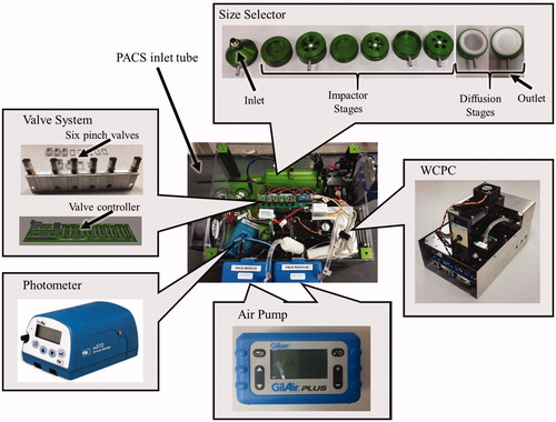
The PACS consists of four main parts (Figure 1): a particle size selector, a valve system, particle detectors (a photometer and water CPC [WCPC]), and controlling software running on a computer. Photographs of the prototype PACS and individual components are shown in Figure 2. Air transports aerosol through an electrically conductive tube to the inlet of the size selector at a flowrate of 0.7 L/min. Six independent valves of the valve system are controlled so that only one is open at a time. The open valve allows aerosol to pass from the inlet through a portion of the machined stages and then to a common manifold. The designed theoretical collection efficiencies by size are shown in Figure S1. We designed the selector to cover aerosols from 10 nm to 10 µm, enabling separation of ultrafine, fine, and coarse mode particles. The aerosol then passes simultaneously to the aerosol detectors, a photometer to measure mass concentrations and a WCPC to measure number concentrations. A full data collection sequence, sampling each size selector stage in turn, yields 12 measurements: six number concentrations and six mass concentrations.

Figure 1. Schematic diagram of the PACS with major components identified.

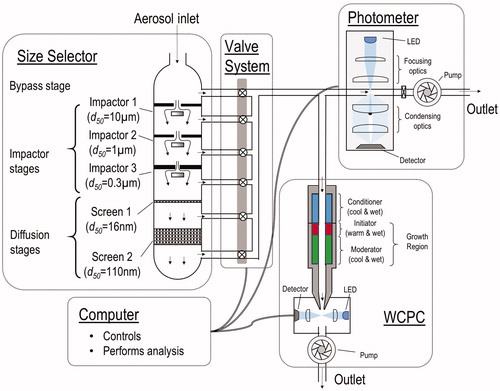
Figure 2. Photographs of the PACS, showing the assembled instrument (center) and each component around the perimeter.

2.1.1. Size selector

The aluminum size selector consists of six stages in a series: a bypass stage, three impactor stages, and two diffusion stages (Figure 2). The first stage allows aerosol entering the inlet to freely pass through to the valve manifold. As shown in Figure S1, the next three stages were designed to collect particles by single-hole impactors with 50% stage cutoff aerodynamic diameters, d₅₀, of 10-µm, 1-µm, and 0.3-µm. These impactors were designed following well-established guidelines in Marple and Willeke (1976). Table S2 lists the dimensions of each impactor stage, including the nozzle width (W), the nozzle length (L), and the distance from impaction plate to nozzle (S). The nozzle width was selected to ensure a jet Reynolds number between 500 and 3,000. For ease of sample recovery, the impaction plates consist of pre-oiled, porous plastic discs (9.5 mm in diameter, Part # 225-388, SKC Inc., Eighty Four, PA, USA) pressed into a recess in the impactor plate assembly. A user can rapidly remove these discs with forceps for later chemical analysis of collected particles. The 1-µm impactor (Stage 2) removes coarse mode particles, allowing fine and ultrafine mode particles to pass; the 0.3-µm impactor (Stage 3) removes particles larger than 0.3 µm, simplifying the interpretation of the diffusion-stage results (Figure S1; solid lines).

The two diffusion stages consist of circular, nylon meshes (41-μm net filters, Part # NY4104700, Carrigtwohill, Co. Cork, Ireland) held in place with a 47-mm filter holder. The meshes collect the smallest particles from the air stream by Brownian motion. Following the theory of a screen-type diffusion battery (Cheng and Yeh 1980), we selected one mesh to provide a d₅₀ of 16 nm of geometric diameter for the first diffusion stage, and six meshes to provide a d₅₀ of 110 nm of geometric diameter for the second diffusion stage (Figure S1; dashed lines). Together, the collection efficiency of the two diffusion stages was designed to match the nanoparticulate matter (NPM) sampling criterion. The NPM criterion was proposed by Cena, Anthony, and Peters (2011) to collect nanoparticles by aerodynamic particle size with an efficiency that mimics their deposition in the human respiratory tract. Since the SMPS measures the particle equivalent mobility diameter, we converted the aerodynamic diameter of NPM to equivalent mobility diameter according to assumed particle density and shape factor from literature (Table S1) shown in online supplemental information (SI).

In theoretical calculations, we assumed standard temperature (20 °C) and pressure (101.3 kPa), standard particle density (1,000 kg/m³), and a hydrodynamic factor of 0.0942. The theoretical penetration curves for impactor stages were calculated with the designed d₅₀ and a sharpness of 1.15, following Hinds (1999). The particles that collect on the impactor and diffusion stages can be analyzed chemically (e.g., digestion followed by elemental analysis) to obtain a time-integrated measure of mass size distributions of various particle compositions, which is the subject of a companion manuscript.

2.1.2. Valve system

The valve system consists of six independent, custom pinch valves and a controller (Figure 2). The valve system, size selector, and manifold are connected by six flexible plastic tubes (length = 46 mm, inner diameter =4.76 mm, outer diameter = 6.35 mm; Tygon R-3603, VWR Scientific Inc., Rochester, NY, USA). The airflow path through the instrument was designed with few bends to minimize particle losses. Since the Bypass Stage contains particles of all sizes, the airflow path flows without bend from the size selector to the photometer, minimizing particle loss from impaction (Figure 1). For other stages, the airflow has two 90° bends as it passes through the valve system and the manifold to the photometer. The airflow passes through an additional four bends on the way to the WCPC.

Each pinch valve includes a motor (Pololu 50:1 micro metal geared motor HP, Pololu Corporation, Las Vegas, NV, USA) connected to the pinch assembly. The direction of the current flow to the motor determines whether the assembly pinches the flexible tube open or closed. The amount of current delivered to the motor controls the magnitude of force applied to pinch the tubing. A custom circuit board designed using Multisim Version 13 (National Instruments Corporation, Austin, TX, USA) uses a microcontroller (Nano, Arduino, Ivrea, Italy) to process serial communications and appropriately signal the six motors through a motor driver (Pololu Dual H-Bridge Motor Driver, DRV8833, Texas Instruments, Dallas, TX, USA). The board also supports the power regulation for all of these components.

2.1.3. Detectors

Two handheld instruments were selected for use as detectors in the PACS: a photometer (SidePak AM510, TSI Inc., Shoreview, MN, USA) and WCPC (Box Magic, Aerosol Dynamics Inc., Berkeley, CA, USA) (Figure 2). Of the 0.7 L/min total flow, 0.4 L/min is directed to the photometer and the remaining 0.3 L/min to the WCPC. The photometer provides a continuous reading (time resolution of 1 s) of mass concentration for aerosols from 0.1 to 10 µm. It uses a 670-nm laser diode to illuminate a portion of the aerosol flow. Set perpendicular to the illumination axis, the photometer’s lens collects light scattered by the particles, focusing the light on a photodetector, which generates a voltage proportional to the mass concentration. The SidePak photometer is portable and widely used to measure aerosol mass concentrations in outdoor and indoor environments (Klepeis, Ott, and Switzer 2007; Jiang et al. 2011).

The laminar-flow WCPC, developed by Hering, Spielman, and Lewis (2014), provides a continuous measurement (time resolution of 1 s) of number concentration up to 10⁷ particles/cm³ for particles from 5 nm to 2 μm. Traditional WCPCs consist of a cool and wet wall (conditioner) followed by a warm and wet wall (growth region) that promotes condensation of water onto airborne particles (Hering et al. 2005). The WCPC used in this study replaces the “warm and wet wall (growth region)” of the traditional WCPC with two sections—a short warm and wet “initiator” (indicated in red in Figure 1) and a cool and wet “moderator” (indicated in green in Figure 1). The “initiator” provides the water vapor that creates the supersaturation, while the “moderator” provides the time for particle growth. As demonstrated by Hering, Spielman, and Lewis (2014) through modeling and laboratory tests, this design reduces the added heat and water vapor while achieving the same peak supersaturation and similar droplet growth as previous WCPC designs. Therefore, the working time can be extended with the same amount of added water by consuming less power. Moreover, the WCPC is portable and operates independent of orientation. Two personal sampling pumps (GilAir PLUS, Gilian Instrument Corporation, Wayne, NJ, USA) provide airflow through the detectors. These external pumps were needed because the original pumps used in the SidePak AM510 and WCPC were not powerful enough to overcome the pressure drop caused by the small impactor nozzle in the size selector (Impactor Stage 3).

2.1.4. Stage penetration by size

We measured the penetration by size and pressure drop of each stage of the separator using the experimental setup shown in Figure 3. Room air was filtered with two high efficiency particulate air filters and passed into a chamber consisting of a mixing zone (0.64 m × 0.64 m × 0.66 m) and a sampling zone (0.53 m × 0.64 m × 0.66 m) divided by a perforated plate (600 evenly spaced 0.6-cm holes). Aerosol was injected into the mixing zone, where a small fan ensured that the aerosol was well mixed, and then passed through the perforated plate to provide a uniformly distributed aerosol in the sampling zone.

Figure 3. Experimental setup used to measure particle penetration by size and pressure drop.

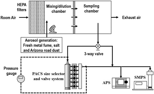
We generated three aerosol types to span the size range of interest. Fresh metal fume was produced with a spark discharge system, providing an ultrafine mode aerosol (Park et al. 2014). A salt aerosol was generated using a Collision-type nebulizer (Aeroneb Solo Model, Aerogen, Martinez, CA, USA) with 0.9% salt solution, providing a fine mode aerosol. Arizona road dust (Fine Grade, Part # 1543094, Powder Technology Inc., Arden Hills, MN, USA) was aerosolized using a fluidized bed aerosol generator (3400A, TSI Inc., Shoreview, MN, USA), providing a coarse mode aerosol. We maintained steady aerosol concentrations (8.2 × 10⁴ ± 2.5 × 10³ particles/cm³ for fresh metal fume, 4.6 × 10⁴ ± 8.7 × 10² particles/cm³ for salt and 4.8 × 10² ± 8.7 particles/cm³ for Arizona road dust) throughout all tests.

We measured particle penetrations by size through each stage for each aerosol type six times (n = 6 stages ×3 aerosol types ×6 replications =108 tests). Particle number concentrations by size were measured alternately entering the PACS and exiting the manifold after passing through the stage being measured. The number concentrations by equivalent mobility particle size were measured with an SMPS (SMPS 3936, TSI Inc., Shoreview, MN, USA) operated with a Nano DMA (DMA 3085, TSI Inc., Shoreview, MN, USA) for 5–20 nm and a long DMA (DMA 3081, TSI Inc., Shoreview, MN, USA) for 28–496 nm. The number concentrations by aerodynamic particle size were also measured with an APS (APS 3321, TSI Inc., Shoreview, MN, USA) for particles larger than 0.7 μm. The flowrate of the SMPS and APS were adjusted to achieve a total flowrate through the PACS of 0.7 L/min. The flowrate of the SMPS was set to 0.3 L/min. Filtered air was supplied at 4.6 L/min to the APS so that it sampled with a flowrate of 0.4 L/min.

The penetration for each size bin of the SMPS and APS was calculated as the number concentration exiting the outlet divided by that entering the inlet. We calculated the sharpness (σ) of the collection efficiency curve of each stage as follows: (1) where d₈₄ and d₅₀ are the particle diameters corresponding to the collection efficiency of 84% and 50%, respectively.

We calculated the R-squared (R²) to evaluate how well the collection efficiency of particles to the meshes of the diffusion stages approximates the NPM curve as follows: (2) where j is the size bin, and are the theoretical and measured NPM data points, respectively, is the averaged collection efficiency over j size bins.

2.1.5. Pressure drop

We measured the pressure drop of each stage three times (n = 6 stages ×3 replicates = 18 tests) with a pressure gauge (Model 407910, 0–200 kPa, Extech Instruments, Nashua, NH, USA) at a flowrate of 0.7 L/min. The pressure gauge was connected between the inlet and outlet of the valve manifold (dashed lines in Figure 3). Cumulative pressure drop was measured across the target stage.

2.1.6. Detector response time after valve switch

We measured the response time to achieve a stable number concentration after a valve switch (n = 6 stages ×3 replications =18 tests). A knowledge of response time is needed to set an appropriate delay before detector concentrations are used in calculations. We measured the response time for each stage using a mixed aerosol of fresh fume, aged metal fume, and Arizona road dust. Fresh fume was produced with a spark discharge system to represent an ultrafine mode. Aged metal fume produced with a second spark discharge system was passed through two coagulation chambers in series (2 coagulation chamber ×200 L = 400 L) to allow the fume to age into a fine mode. Arizona road dust was aerosolized using a fluidized bed aerosol generator to represent the coarse mode. This mixed aerosol was injected into the mixing/dilution chamber (Figure 3). The valves of the size selector were opened sequentially for 30 s one at a time. For each stage, the response time was measured as the time to reach 95% of the steady-state number concentration by the WCPC after the valve for that stage was opened.

2.2. PACS software

A custom software program was developed using Visual Basic (VB.Net Version, Microsoft Corporation, Redmond, WA, USA) to control the timing of valves and to acquire data from the photometer and WCPC. The user defines the delay after a valve is opened and the duration over which concentrations are averaged (15 s in the current work). The program sequentially opens one valve at a time, collecting and storing six mean number concentrations and six mean mass concentrations for a single scan through all stages (3 min in the current work). It then calls a MMLN fitting algorithm to translate these 12 measurements into aerosol size distributions of number, surface area, and mass concentration. The program then displays these data graphically and numerically by particle size mode to the user.

2.2.1. Description of the algorithm

A flowchart of the fitting algorithm developed to determine the continuous aerosol size distributions of number (N), surface area (SA), and mass (M) concentrations from PACS is shown in Figure S3. The inputs are the six observed number concentrations (N_obs,k) and six observed mass concentrations (M_obs,k) in each stage k (k = 0–5) of the size selector obtained from one cycle of the PACS measurement. We used a tri-modal, log-normal distribution to mathematically express an aerosol (Hussein et al. 2005): (3) where i is the aerosol mode (i = 1 represents the ultrafine mode, i = 2 represents the fine mode, and i = 3 represents the coarse mode); N is the number concentration; CMD is the count median diameter; GSD is the geometric standard deviation; and d_p is the aerodynamic particle diameter.

In Step 1, we estimate N_i, GSD_i and CMD_i by a grid-search process. For GSD, we set the step size to 0.1 independent of mode and the range as follows: ultrafine mode between 1.5 and 1.8; fine mode between 1.8 and 2.2; and coarse mode between 2.1 and 2.7. For CMD, we set the step size and range as follows: ultrafine mode between 5 and 40 nm with a step size of 5 nm; fine mode between 40 and 200 nm with a step size of 50 nm; and coarse mode between 0.4 and 2 μm with a step size of 0.5 μm. These ranges were selected to encompass diverse aerosols reported on by Whitby and Sverdrup (1980).

For simplicity, we re-write Equation (3)(3) as two equations: (4) (5) where is a frequency distribution of an aerosol mode i. Using an optimization method described by Hussein et al. (2005), we estimate the number concentration in each mode (N_i) using number and mass concentration measurements. We calculate the squared error between observed (N_obs,k) and fitting number concentration (N_fit,k), and then set the partial derivative of the square effort with respect to N_i to zero (Equation (6)(6) ): (6) where N_fit,k is the number concentration fit by the algorithm in each PACS stage k. For the first stage, N_fit,k is calculated as: (7)

For subsequent stages, N_fit,k is computed as the penetration through the previous stage, P_k−1, multiplied by the number concentration entering the previous stage: (8)

We also set the partial derivative of the squared difference between observed (M_obs,k) and fitting mass concentration (M_fit,k) with respect to N_i to zero (Equation (9)(9) ): (9) where M_fit,k is the mass concentration fit by the algorithm in each PACS stage k. For the first stage, M_fit,k is calculated as: (10) where m_i is the mass of one particle with the size of averaged mass diameter (AMD_i) in mode i. To calculate m_i, the Hatch–Choate equation (Hinds, 1999) is applied to convert CMD_i to the particle diameter associated with the average mass of all particles in a mode (AMD_i) as: (11) (12) where ρ is the particle density.

For subsequent stages, M_fit,k is computed as the penetration through the previous stage, P_k−1, multiplied by the mass concentration entering the previous stage: (13)

We applied the CLLS solver, lsqlin, in MATLAB (MATLAB R2014a, The MathWorks Inc., Natick, MA, USA) to solve for N_i, using the 12 linear equations (Eqs. (5)(5) , (6)(6) , (8)(8) , and (11)) as equality constraints. A constraint of N_i > 0 is added to prevent obtaining negative values of N_i.

We then calculate bias of number and mass concentration in each PACS stage k as and , respectively. The log-normal parameters (N_i, CMD_i, and GSD_i) are saved when the bias in each stage are smaller than a certain tolerance (i.e., within ±10% for the first stage, ±50% for the second stage, and ±100% for other stages). The Environmental Protection Agency (EPA) and National Institute for Occupational Safety and Health (NIOSH) specified that the acceptance criteria of percent bias should be within ±10% (EPA 2006; NIOSH 2012). Therefore, the ±10% tolerance for the first stage ensures that the number and mass concentrations measured by the PACS meet these acceptance criteria. After completing the grid-search ranges of GSD_i and CMD_i, the averaged GSD_i and CMD_i are calculated from saved values.

In Step 2, we refine the estimates of N_i, GSD_i and CMD_i by narrowing the grid-search ranges of GSD_i and CMD_i, and decreasing the step size of CMD_i. Then Step 1 is repeated until the step size of CMD_i equals 0.1 × 10ⁱ nm (i.e., 1 nm for ultrafine mode, 10 nm for fine mode, and 100 nm for coarse mode). We estimate the log-normal parameters (N_i, CMD_i, and GSD_i) by minimizing the sum of the squared relative errors (SSREs) between the measurements and fitting results (2 measurements [N and M] × 6 stages =12 SSREs). (14)

Then, we applied the Hatch-Choate equation to convert CMD_i and GSD_i to the surface area median diameter (SMD_i) and mass median diameter (MMD_i) as: (15) (16)

Lastly, for each metric (N, SA, and M), the algorithm outputs: (1) aerosol size distribution from 10 nm to 10 µm resolved in 40 size bins for each decade of data; (2) summary statistics (CMD, SMD, MMD, GSD, N, SA, M) for each mode.

2.2.2. Algorithm refinement

We conducted tests to determine the step size and range for the grid-search of CMD_i that provides accurate and precise size distributions for four pre-defined typical atmospheric aerosols (including clean continental background, urban and freeway, coal power plant and marine surface aerosols, see Table S2). These four pre-defined aerosols were selected from Whitby and Sverdrup (1980) to encompass a wide range of size distributions encountered in the atmosphere. For example, the clean continental background aerosol was used to test the accuracy of the algorithm under low concentrations of aerosols in all three modes (1,900 #/cm³). For the urban and freeway aerosols, the number concentration of the ultrafine mode was high (1.9 × 10⁶ #/cm³), the surface area concentrations of the ultrafine mode (2.0 × 10⁹ µm²/m³) and fine mode (1.1 × 10⁹ µm²/m³) were similar, and the mass concentrations of the fine mode (38 µg/m³) and coarse mode (43 µg/m³) were also similar. For the coal power plant aerosol, the surface area concentration of the fine mode (5.1 × 10⁸ µm²/m³) was much higher than that of the ultrafine mode (4.3 × 10⁷ µm²/m³) and the coarse mode (4.0 × 10⁷ µm²/m³). For the marine aerosol, the number concentration was only 440 #/cm³; however, the mass concentration was over 12 µg/cm³.

For each aerosol, we used the nine parameters (one CMD × three modes + one GSD × three modes + one N × three modes = nine parameters) provided by Whitby and Sverdrup (1980) to obtain the 12 equivalent values that would be measured with the PACS (six N_obs,k, and six M_obs,k) assuming standard density (1,000 kg/m³) and spheres (shape factor =1). We summarized the inputs in Table S3.

We evaluated the influence of the grid-search step size on the accuracy and precision of the fit for the four aerosols. For CMD_i, the step size was changed from 0.1 × 10ⁱ nm to 0.5 × 10ⁱ nm for each mode i with an increment of 0.05 × 10ⁱ nm. For example, the step size was changed from 1 to 5 nm for ultrafine mode (i = 1) with an increment of 0.5 nm, from 10 to 50 nm for fine mode (i = 2) with an increment of 5 nm, and from 100 to 500 nm for coarse mode (i = 3) with an increment of 50 nm. We calculated three statistical parameters: the normalized mean bias (NMB), normalized mean error (NME), and the R-squared (R²) values as follows: (17) (18) (19) where and are the fitting and real aerosol size distribution, respectively, for each size bin, j. is the averaged value over all size bins. In this study, we used 40 size bins for each decade of data (e.g., 40 bins from 10 to 100 nm).

NMB indicates the tendency of the algorithm to over-predict or under-predict variables, although the summing of positive and negative biases can lead to cancelation of an absolute magnitude of discrepancies. We also calculated NME, the sum of the absolute values of NMB at each size bin, to provide another indicator without the cancelation problem. In addition, R² was used to indicate how well the fitted tri-modal log-normal distribution approximated the real data points. We used the mean of each statistical parameter (NMBs, NMEs and R²s) for the four aerosols tested to represent the accuracy, and the standard deviation (SD) of each parameter to represent the precision of the fit.

According to the above testing results, we selected the step size with the most accurate and precise fit. However, the computation time would dramatically increase due to the increase of grid-search times of CMD_i with decreased step size. In order to decrease the computation time, we established narrowed grid-search ranges for GSD_i and CMD_i with each decrease in the step size of CMD_i.

We then evaluated the refined algorithm for the four typical atmospheric aerosols by comparing the fitting results to the observed ones as follows: (1) we compared the aerosol size distributions in three metrics, (2) we compared the nine parameters given by Whitby and Sverdrup (1980), and (3) we calculated the statistical parameters (NMB, NME, and R²) in three metrics.

2.2.3. Sensitivity analysis

We performed a sensitivity analysis to test the robustness of the algorithm in the presence of uncertainties arising due to unknown particle density and shape factor. The sensitivity study was conducted by changing the particle density from 500 to 3,000 kg/m³ with a step of 100 kg/m³, and the shape factor from 1 to 3 with a step of 0.1. Therefore, 546 combinations (26 densities ×21 shape factors) of density and shape factor were selected to cover a wide range of aerosol types found in different environments. For example, the density of diesel fume ranges from 500 to 1,200 kg/m³ (Park, Kittelson, and McMurry 2004). The density of welding fumes is over 3,000 kg/m³ (Kim et al. 2009). The shape factor of salt aerosol is 1.08 (near spherical), whereas that for welding fume can reach over 3 (Kim et al., 2009). For each combination of density and shape factor, we followed the same procedure described in Section 2.2 by calculating the statistical parameters (NMB, NME, and R²) in three metrics for each of the four aerosols.

3. Results and discussion

3.1. PACS hardware

3.1.1. Impactor stages

Particle penetrations by aerodynamic particle size for bypass and impactor stages, and geometric particle size for diffusion stages are shown in Figure 4 and summarized in Table 1. The SMPS measures the equivalent mobility diameter, which was converted to aerodynamic diameter using assumed particle densities and shape factors shown in Table S1. In all stages, diffusion losses were observed for small particles (<∼37 nm), and gravitational settling/impaction/interception losses were observed for large particles (>∼0.5 µm). For example, for the Bypass Stage (Figure 4a), the maximum penetration (∼100 ± 3%) was observed for aerosols with diameters from ∼37 to ∼0.5 µm. For particles progressively smaller than ∼36 nm, the penetration gradually decreased to ∼58% (±4%) for ∼12 nm particles due to diffusion losses. For particles larger than ∼0.5 µm, the penetration gradually decreased to ∼72% (±15%) for ∼7 µm particles due to gravitational settling and impaction.

Figure 4. Fractional penetration measured for the six PACS stages (error bars represent the standard deviation of six measurements; dashed line indicates the measured d₅₀).

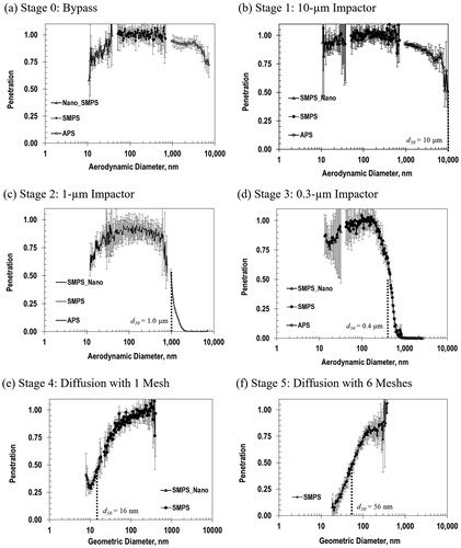
Table 1. Physical characteristics, flow parameters, and experimental results for the impactor stages.

Stage	Physical characteristics			Flow parameters		Design	Experimental results
	W (mm)	L (mm)	S/W	Re	V (cm/s)	d50 (µm)	d50 (µm)	Stk50	σ	ΔP (kPa)	Response (s)
Bypass Stage 0	n.a.	n.a.	n.a.	n.a.	n.a.	n.a.	n.a.	n.a.	n.a.	0	15 ± 4
Impactor Stage 1	3.15	4.47	2.78	313	150	10^a	∼10^a	0.22	2.6	0	7 ± 1
Impactor Stage 2	0.67	2.70	6.81	1470	3309	1.0^a	1.0^a	0.22	1.6	0.65	10 ± 1
Impactor Stage 3	0.48	0.48	5.67	2051	6447	0.3^a	0.4^a	0.22	1.5	2.88	8 ± 2
Diffusion Stage 4	n.a.	n.a.	n.a.	25	n.a.	0.016^b	0.016^b	n.a.	n.a.	2.88	8 ± 1
Diffusion Stage 5	n.a.	n.a.	n.a.	25	n.a.	0.110^b	0.056^b	n.a.	n.a.	2.88	6 ± 0

W: the nozzle width; L: the nozzle length; S: the distance from impaction plate to nozzle; Re: Reynolds number; d₅₀: 50% stage cutoff diameter; Stk₅₀: Stokes number at 50% collection efficiency; σ: curve sharpness; ΔP: cumulative pressure drop; V: nozzle velocity; a: aerodynamic diameter; b: geometric diameter; n.a.: not applicable.

For particles progressively smaller than ∼37 nm, the penetration of the 10-µm impactor (Stage 1, Figure 4b), gradually decreased from ∼100% (±10%) to ∼88% (±7%) for ∼12 nm particles due to diffusion losses. The characteristic d₅₀ of the Impactor Stage 1 was estimated to be ∼10 µm of aerodynamic diameter with the σ of 2.6 (Table 1). More particle losses from diffusion were observed in the 1-µm impactor (Impactor Stage 2) than in the 10-µm impactor. For particles progressively smaller than ∼37 nm, the penetration gradually decreased from ∼90% (±18%) to ∼55% (±5%) for ∼12 nm particles (Figure 4c). The d₅₀ of Impactor Stage 2 was ∼1.0 µm of aerodynamic diameter with the σ of 1.6 (Table 1). In Impactor Stage 3 (Figure 4d), the penetration gradually decreased from ∼100% (±11%) to ∼76% (±9%) for particles from ∼116 to ∼18 nm. The d₅₀ of this impactor was ∼0.4 µm of aerodynamic diameter with the σ of 1.5 (Table 1). The Bypass Stage provided a collection efficiency curve similar to that of the 10-µm impactor and could potentially be eliminated in future versions of the PACS.

As expected, the measured characteristic d₅₀ of each impactor stage was similar to the design (Table 1). The measured d₅₀ (0.4 µm) of Impactor Stage 2 was slightly larger than the designed one (0.3 µm). The penetration curve of the last impactor stage was sufficiently sharp (σ = 1.5) to remove airborne particles larger than the ∼400 nm, which would introduce uncertainties in data interpretation with the diffusion stages. This sharpness is sharper than a commercial nanosampler sold by KANOMAX (σ = 1.9) (KANOMAX, 2012) and similar to others, such as a personal nanoparticle respiratory deposition sampler (σ = 1.53) (Cena, Anthony, and Peters 2011) and an Anderson cascade impactor using inertial filter technology (σ = 1.6) (Hata et al. 2012). It was less sharp than that of either a personal nanoparticle sampler (σ = 1.3) (Tsai et al. 2012) or a microorifice uniform deposit impactor (σ = 1.2) (Chen et al. 2016). Although high flowrates and low pressures are able to achieve sharper curves and reduce diffusion loss than in this study, they require large pumps which make the device less portable (Marple, Rubow, and Olson 2001).

A knowledge of actual aerosol penetration by size in each stage is important to reduce uncertainties in estimating aerosol size distributions from PACS data. Shi, Khan, and Harrison (1999) showed that particle loss caused by diffusion of ultrafine mode particles should be considered to obtain accurate aerosol size distributions with the SMPS. Reineking and Porstendörfer (1986) stressed that particle losses should be incorporated in analysis routines to correct the raw measurements for any aerosol measurement instrument. In the development of the inversion algorithm, we used the observed penetration of each stage, which account for particle losses through the PACS, to retrieve the particle size distributions.

The particle losses we observed for the impactor stages are similar to those observed for other impactors. According to theory, particle losses occur due to gravitational settling, impaction, interception and diffusion (Hinds 1999). Marple, Rubow, and Behm (1991) studied the inter-stage losses within the MOUDI, reporting that the losses were the greatest for the larger particles (∼15 µm), where the gravitational settling and impaction were most severe. However, the losses rapidly decreased with progressive smaller particles to negligible particles less than 5 µm. The losses increased again as the particle size reached ∼100 nm due to the diffusional effects of these small aerosols.

3.1.2. Diffusion stages

Penetration by geometric particle size for the diffusion stages are shown in Figures 4e and 5f. Since most of particles (97 ± 3%) larger than 400 nm were removed by the Impactor Stage 3 (Figure 4d), only particles smaller than 500 nm are shown in Figures 4e and 5f. For the first diffusion stage with one mesh (Stage 4, Figure 4e), penetration was highest (99 ± 7%) for particles from ∼300 nm to 400 nm and gradually decreased with decreasing particle size (<40% for particles smaller than 10 nm). The measured d₅₀ of the first diffusion stage was ∼16 nm of geometric diameter (Table 1). For the second diffusion stage with 6 meshes (Stage 5, Figure 4f), penetration gradually decreased from ∼100% for particles of ∼400 nm to ∼8% for particles of ∼15 nm. The measured d₅₀ of the second diffusion stage was ∼56 nm of geometric diameter (Table 1). As expected, the measured characteristic d₅₀ of each diffusion stage was similar to the design. The penetrations in diffusion stages can be used to provide size information for particles less than 300 nm. In the last stage, since less than 10% of particles smaller than 10 nm can penetrate the six meshes, the lower size limit of the PACS measurement was set at 10 nm.

The effective collection efficiency by equivalent mobility particle size of particles to the two diffusion stages combined (stages 4 and 5) is shown in Figure S2 (black dots). The collection efficiency was lowest (15 ± 10%) for ∼300 nm particles, where the last impactor collects the particles larger than this size, and gradually increased with decreasing particle size. This combined collection efficiency is similar to the NPM sampling criterion (solid line) with R² of 0.97. This criterion represents the deposition of nanoparticles in the human respiratory tract (Cena, Anthony, and Peters 2011). Thus, the mass of aerosols chemically analyzed on the two diffusion stages can be added to estimate the nanoparticles that deposit in human respiratory system. Few examples of samplers with efficiencies matching respiratory deposition can be found in literature. The size-selective inlet, multistage sampler and NRD sampler were designed to mimic a modified ICRP lung deposition fraction (Kuo et al. 2005; Koehler, Clark, and Volckens 2009; Cena, Anthony, and Peters 2011).

3.1.3. Pressure drop

The measured cumulative pressure drop for each PACS stage is listed in Table 1. The highest pressure drop (2.23 kPa) was caused by the third impactor, followed by the second impactor (0.65 kPa). The pressure drop caused by other stages was negligible (∼0 kPa). Overcoming the system pressure drop is critical to maintaining a stable flowrate. The pumps originally used in the photometer and WCPC were unable to maintain the design flowrate of 0.7 L/min due to the pressure drop imparted by the 300-nm impactor. The external air pumps (the portable GilAir PLUS air pumps) used in the final PACS design are able to overcome this pressure drop without faulting due to low system flowrate requirement. These external pumps can be replaced with a single pump internal to the PACS in future versions.

3.1.4. Detector response time after valve switch

The number and mass concentrations of the combined test aerosol measured by the detectors after passing through each stage are shown in Figure 5. The time to achieve 95–105% of steady-state number concentrations for each stage is shown in Table 1. As expected, the number concentration was more stable than the mass concentration because the metal fume generated by the spark system is more stable than the Arizona road dust generated by the fluidized bed aerosol generator. For the Bypass Stage, the number concentration went above steady-state because of the transition from the high pressure drop downstream of the 300-nm impactor to the low pressure drop of the Bypass Stage. This larger pressure change caused the air flowrate to become higher than 0.7 L/min, thereby causing the WCPC to erroneously read higher concentrations. As a result, the Bypass Stage had the longest response time (15 ± 4 s). The response time of Stage 1 (7 ± 1 s) was ∼50% faster than that of the Bypass Stage, because there was little pressure drop in this stage. Due to the pressure drop added by Stages 2 and 3, the WCPC response time increased by a few seconds (totaling 10 ± 1 s for Stage 2 and 8 ± 2 s for Stage 3). For the two diffusion stages (Stage 4 and 5), the WCPC response times were 8 ± 1 s and 6 ± 0 s, respectively.

Figure 5. Number concentrations from the WCPC (a) and mass concentrations from the photometer (b) for the combined aerosols of fresh metal fume, aged metal fume and ARD (error bars represent the standard deviation of three measurements).

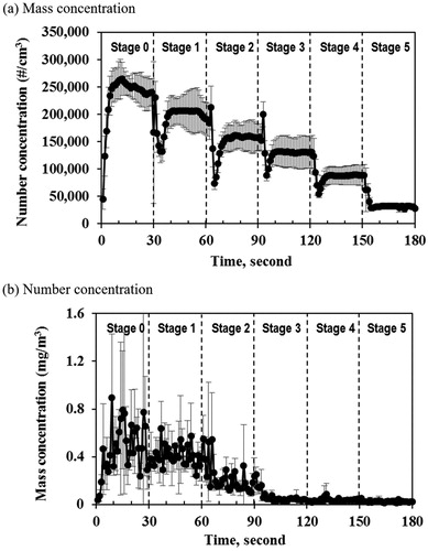
There are three factors for determining the response time: (1) opening and closing valves; (2) response of the pumps to recover from pressure drop released by the stage; and (3) the clearing of the volume of air between the exit of the stage and the detector. Valve opening and closing is fairly rapid (∼3 s), so unlikely to be the largest contributor to overall response time. The time for the pumps to regain airflow is dependent on the pressure drop added/released by stage. Based on the airflow and the air volume between the exit of the stage and the WCPC, the estimated time for clearing the volume of air between the exit of the stage and the detector is ∼3 s for the Bypass Stage, ∼3.1 s for the Stage 1, ∼3.3 s for the Stage 2, ∼3.4 s for the Stage 3, ∼3.4 s for the Stage 4, and ∼3.5 s for the Stage 5.

These time delays and the associated averaging time define the minimum time required to obtain a full set of measurements with the PACS. If the averaging time is 15 s, then the minimum time required to obtain a set of measurements over all stages was 144 s.

3.2. PACS software

3.2.1. Algorithm refinement

In general, decreasing the step size of CMD_i improved accuracy and precision of the fitting results (Figure 6). Independent of step size, most mean NMBs were near zero (within ±3.6%), except surface area concentration (Figure 6a). The mean and SD of NMBs for surface area concentrations oscillated with decreasing step size becoming stable for the smallest step size. The surface area concentration was underestimated for the coarsest step size (NMB of −4.3 ± 11.7%), although it was near zero (1.8 ± 2.7%) for the smallest step size. The mean and SD of NMEs decreased substantially with decreasing step size (Figure 6b). For number concentrations, NMEs decreased from 26.8 ± 14.7% for a step size of 0.5 × 10ⁱ nm to 9.7 ± 4.0% for a step size of 0.1 × 10ⁱ nm (Figure 6b). For mass concentration, NME reached the highest value of 39.1 ± 43.3% for a step size of 0.5 × 10ⁱ nm and then decreased to 8.0 ± 4.3% for a step size of 0.1 × 10ⁱ nm. For all metrics, the mean of R² approached one (0.97 for N, 0.94 for SA, and 0.98 for M), and the SD of R²s reached was near zero (0.04 for N, 0.07 for SA, and 0.02 for M) for the smallest step size of 0.1 × 10ⁱ nm (Figure 6c). For number concentration, R² increased from 0.91 ± 0.08 for a step size of 0.5 × 10ⁱ nm to 0.97 ± 0.04 for a step size of 0.1 × 10ⁱ nm. For surface area and mass concentrations, decreasing the step size from 0.5 × 10ⁱ to 0.1 × 10ⁱ nm increased the R² from 0.89 ± 0.16 to 0.94 ± 0.07, and from 0.44 ± 1.09 to 0.98 ± 0.02, respectively.

Figure 6. Effect of the grid-search step size on the fitting results expressed as: (a) NMB; (b) NME; (c) R². The step size ranged from 1 nm to 5 nm for ultrafine mode, from 10 nm to 50 nm for fine mode, and from 100 nm to 500 nm for coarse mode. Error bars represent one standard deviation.

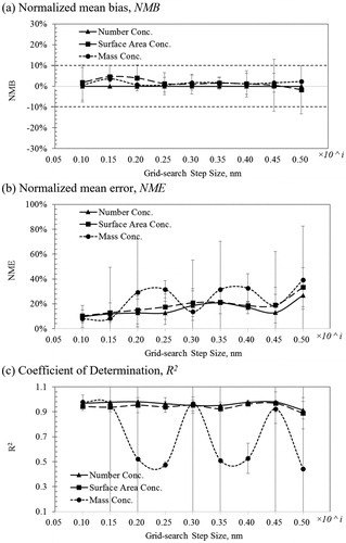
We selected 0.1 × 10ⁱ nm as the final step size in the algorithm for several reasons. For each of the three statistical parameters, we found the most accurate and precise estimates at the step size of 0.1 × 10ⁱ nm. The results of NMB indicated that the smallest step size resulted in the most accurate (with 0.8% of mean of NMBs) and precise (with 1.4% of SD of NMBs) fit for all three metrics. Similar to NMB, the NME results also indicated that the smallest step size resulted in the most accurate (with 9.3% of mean of NMEs) and precise (with 4.6% of SD of NMEs) fit for all three metrics. For R², the smallest step size resulted in the most accurate (with 0.96 of mean of R²) and precise (with 0.04 of SD of R²) fit for all three metrics as well. The oscillations of fitting results using various step sizes might be caused by the value of the last two significant figures of observed CMD_i. If the observed value of CMD_i could be located during grid-search, the fitting results would be accurate. The smaller the step size in the algorithm, the better chance he algorithm has of finding the observed value. However, using a computer with a processor of i7-4790 CPU (3.60 GHz) and installed memory of 8.00 GB, the computation time increased from 1.7 ± 1.0 s for a step size of 0.5 × 10ⁱ nm to 43.3 ± 29.0 min for a step size of 0.1 × 10ⁱ nm.

We refined the algorithm using an adaptive process to decrease the computation time while still using the smallest step size for CMD_i (0.1 × 10ⁱ nm). Further investigation of the above test results indicated that, regardless of CMD_i step size, fitted GSD_i were within ±0.2 and fitted CMD_i were within ±0.5 × 10ⁱ nm of true values. Thus, the grid-search ranges could be narrowed for each pass through Step 2 of the algorithm to minimize search times without sacrificing accuracy. We grid-searched GSD_i within the range of ±0.2 constrained to the best values of GSD_i obtained from Step 1, which applied the whole range of GSD_i. Similarly, we grid-searched CMD_i within aerosol diameter ranges of ±0.5 × 10ⁱ nm constrained around the best values of CMD_i obtained from Step 1. The step size of CMD_i was decreased from 0.5 × 10ⁱ to 0.3 × 10ⁱ nm, and then to 0.1 × 10ⁱ nm with narrowed ranges of GSD_i and CMD_i to refine the algorithm. The computation time with the grid-search was 24.3 ± 11.4 s compared to 43.3 ± 29.0 min without the refinement.

The results of fitting aerosol size distributions using the refined algorithm are shown in Figure 7 and summarized in Table 2. Overall, the fitted and observed aerosol size distributions in three metrics (number, surface area, and mass concentrations) were in close agreement for all four pre-defined aerosols. For the ultrafine and fine modes, the algorithm found almost the exact values of the CMD_i, GSD_i, and N_i for all four aerosols. The largest discrepancies between fit and observed values occurred for the fine and coarse mode of mass concentration for coal power plant aerosol (Figure 7c). The fitted distribution was shifted to larger sizes for both fine and coarse mode. For the surface area concentration of coal power plant aerosol, the algorithm underestimated the fine and coarse modes (Figure 7c). For the coarse mode, the CMD₃ was overestimated, and GSD₃ was underestimated to compensate for the overestimation of the aerosol size (CMD₃).

Figure 7. Particle size distributions estimated with the PACS fitting algorithm for four atmospheric aerosols: (a) clean continental background; (b) urban and freeway; (c) coal power plant; (d) marine surface. The dotted lines (black) represent the pre-defined aerosol, and the solid lines (red) represent the distribution fit with the algorithm.

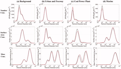
Table 2. Summary of fitting results for aerosols found in diverse environments, assuming standard density spheres.

Aerosol type	, %			, %
	N	SA	M	N	SA	M	N	SA	M
1. Clean background	0.0	3.5	0.0	11.9	6.2	3.3	0.98	1.00	1.00
2. Urban and freeway	0.0	−3.2	0.0	5.3	7.9	9.4	1.00	0.99	0.99
3. Coal power plant	0.0	−4.9	0.0	27.6	24.0	23.2	0.90	0.94	0.90
4. Marine surface	0.0	2.5	−2.7	17.5	6.2	5.9	0.97	0.99	1.00

NMB: normalized mean bias; NME: normalized mean error; N: number concentration; SA: surface area concentration; M: mass concentration.

Table 2 summarizes the performance statistics of the refined algorithm for the four pre-defined aerosols. According to the NME and R² values, the number aerosol size distribution was the most accurate among the three metrics. The estimated number and mass concentrations were more accurate than the surface area concentrations. For all four aerosols, NMBs for both number and mass concentrations were within ±0.2%. The estimations of surface area concentrations were not as good as number and mass concentrations. The percentage bias between fitted and observed size distributions for number and mass concentrations meets the acceptable criteria from both the EPA and NIOSH (within ±10%).

3.2.2. Sensitivity analysis

The results of the sensitivity study are depicted in Figure S4. For all parameters (NMB, NME, R²), the fitting of surface area concentrations was more sensitive to unknown density and shape factor than number and mass concentrations. The NMBs of number and mass concentrations were ±10%, whereas those for surface area concentrations deviated substantially above zero (underestimation of concentration) for particle density less than 1,000 kg/m³, and below zero (overestimation of concentration) for particle density larger than 1,000 kg/m³. In addition, by increasing the shape factor, the algorithm tended to underestimate the surface area concentration (Figure S4a).

NME and R² plots are shown in Figure S4b and S4c, respectively. For all metrics, aerosol size distributions fit well (low NME and high R² values) if the density and shape factor increased simultaneously. For aerosol number size distributions, the algorithm was most accurate (NMEs of 36.2 ± 22.8% coupled with R²s of 0.80 ± 0.25) for the urban and freeway aerosol, followed by the marine surface aerosol (NMEs of 45.0 ± 34.4% and R²s of 0.67 ± 0.58), coal power plant aerosol (NMEs of 47.1 ± 29.5% and R²s of 0.68 ± 0.48) and background aerosol (NMEs of 61.2 ± 23.3% and R²s of 0.35 ± 0.45). For aerosol surface area size distributions, the algorithm was most accurate for the urban and freeway aerosol, which had the NMEs of 74.7 ± 31.4% and R²s of 0.12 ± 0.68. For aerosol mass size distributions, the algorithm was the most accurate for the marine surface aerosol (NMEs of 26.5 ± 14.0% and R²s of 0.90 ± 0.12). In the marine surface aerosol, both surface area and mass concentrations were dominated by coarse mode.

Independent of particle density and shape factor, fitted number and mass concentrations were within ±10% of known concentrations, a typical acceptance criterion used by EPA and NIOSH (see number and mass concentration plots in Figure S4a, in which, the light green color indicates the bias of approximately 0%). Compared to the number and mass concentrations, the fitted surface area concentrations were more sensitive to changes in particle density and shape factor. Moreover, the aerosol size distributions in all three metrics were fitted relatively well if the density and shape factor increased simultaneously. Density and shape factor are difficult to obtain during field sampling. However, the PACS is able to collect particles on impactor plates in impactor stages, and meshes in diffusion stages. Estimates of particle density can be made based on chemical analysis of collected particles and those of shape factor can be made based on electron microscopy.

3.3. PACS in context of commercial instruments

In a single portable instrument, the PACS provides a way to continuously measure aerosol size distributions of number, surface area, and mass concentration over a wide size range while simultaneously collecting particles with impactor and diffusion stages for chemical analysis. The ELPI, an instrument that retails for ∼$120,000, is the only other single instrument with similar capabilities. However, the low pressure impactor stages used to achieve separation of sub-300-nm particles of the ELPI are expensive to manufacture and require a large, heavy vacuum pump, which dramatically reduces the portability of the system. The reliance on diffusion stages to separate these sized particles in the PACS dramatically reduces the cost of size separation and eliminates the need for high vacuum pumps, thereby promoting portability. We envision that the size selector in future versions of the PACS can be made by injection molding of conductive plastic. ++Further reducing weight and cost. Whereas the ELPI relies on highly sensitive electrometers to measure the concentration of particles, the detectors employed in the PACS (a photometer and a WCPC) are substantially less inexpensive and have been shown robust in field use. Moreover, we envision that these detectors could be combined in a commercial PACS version, further reducing costs associated with redundant user interfaces and pumps.

Similar information can also be obtained with multiple research-grade instruments, such as the combination of an SMPS, APS, and nanoMOUDI (∼$150,000 in total). Researchers combine the SMPS and APS to measure aerosol size distributions over a wide range (Harrison et al. 2000). The wide range aerosol spectrometer (WRAS, Grimm Technologies Inc., Douglasville, GA, USA) combines the portable aerosol spectrometer, differential mobility analyzer, and CPC to measure aerosol size distributions from ∼5 nm to ∼32 µm. The wide-range particle spectrometer (WPS^TM) introduced by Liu et al. (2010) can measure aerosol size distributions from ∼10 nm to ∼10 µm by combining a scanning mobility spectrometer (SMS) and a laser particle spectrometer (LPS). The NanoScan SMPS can measure particle size distributions from 10 to 420 nm in one minute, and the size range can be extended to coarse particles with the Optical Particle Sizer (Tritscher et al. 2013). These systems lack the ability to collect particles for chemical analysis, thereby requiring another instrument like the nanoMOUDI. In addition, the particles deposit on the PACS diffusion stages can be analyzed to determine the nanoparticles that deposit in human respiratory system.

Nevertheless, the PACS also has some limitations that constrain its intended use to measure continuous aerosol size distributions. As shown in Figure 6, 180 s is required for one measurement using the current prototype. If the aerosol concentrations are rapidly changing at the measurement site, the aerosol size distribution measurements might not be accurate. The flowrate is only 0.7 L/min, which might require a long time sampling to collect sufficient particles on the substrates to be detectable. An alternative scheme of reducing the sampling time is to measure the number and mass concentrations in all stages simultaneously by including additional detectors to the outlet of each stage. We did not measure the mass of particles collected on the substrates. This information, however, can be used to calibrate the photometer measurement to further improve the algorithm fitting results.

4. Conclusion

In this article, we described the development of hardware and software of a Portable Aerosol Collector and Spectrometer, the PACS. The PACS continuously measures aerosol size distributions by number, surface area and mass concentrations over a wide size range (from 10 nm to 10 µm), and collect particles with impactor and diffusion stages for post-sampling chemical analyses. The penetration by size in all six stages were measured experimentally to have characteristic d₅₀ (aerodynamic diameter for impactor stages and geometric diameter for diffusion stages) similar to the design. The deposition to the two diffusion stages was in agreement with the NPM sampling criterion. The pressure drop of each stage was sufficiently low to permit its operation with portable air pumps. In the current configuration, the number and mass concentrations from all six stages can be measured in approximately 180 s.

We then developed an MMLN fitting algorithm to rapidly (<3 min) estimate aerosol size distributions in three metrics (number, surface area and mass concentration) with high resolution over a wide size range (from 10 nm to 10 µm) from number and mass concentrations measured with relatively inexpensive handheld detectors in the PACS. Fitted size distributions were in close agreement with observed distributions for all three metrics (number, surface area and mass concentrations) for aerosols found in highly diverse environments. The sensitivity studies indicated that the particle density and shape factor were of great importance to the fitting accuracy of the algorithm. These parameters can be estimated from physical and chemical analysis of particles collected with the size separator of the PACS. With the data analysis methods introduced, the PACS can provide novel exposure assessments, including aerosol size distributions of number, surface area and mass concentrations in a wide size range (from 10 nm to 10 µm). It also provides a way to collect particles to determine time- and mass-weighted size distributions.

Acknowledgments

The authors greatly appreciate the technical support of Drs. Beau Farmer of TSI who provided the photometer and Susanne V. Hering of Aerosol Dynamics who provided the WCPC.

Additional information

Funding

This work was supported by the small-business innovative research (SBIR) project (AF131-024) from the U.S. Air Force and a pilot project from the Heartland Center for Occupational Health & Safety (NIOSH T42OH008491). Some of the equipment used to conduct the study was borrowed from the Exposure Assessment and Modelling Facility of the University of Iowa Environmental Health Sciences Research Center (NIEHS/NIH P30 ES005605).

References

- Abt, E., H. H. Suh, G. Allen, and P. Koutrakis. 2000. Characterization of indoor particle sources: A study conducted in the metropolitan Boston area. Environ. Health Perspect. 108 (1):35.
- Baron, P. A. 1986. Calibration and use of the aerodynamic particle sizer (APS 3300). Aerosol Sci. Technol. 5 (1):55–67.
- Brouwer, D. H., J. H. Gijsbers, and M. W. Lurvink. 2004. Personal exposure to ultrafine particles in the workplace: Exploring sampling techniques and strategies. Ann. Occup. Hyg. 48 (5):439–453.
- Brunekreef, B., and B. Forsberg. 2005. Epidemiological evidence of effects of coarse airborne particles on health. Eur. Respir. J. 26 (2):309–318.
- Cena, L. G., T. R. Anthony, and T. M. Peters. 2011. A personal nanoparticle respiratory deposition (NRD) sampler. Environ. Sci. Technol. 45 (15):6483–6490.
- Chen, M., F. J. Romay, L. Li, A. Naqwi, and V. A. Marple. 2016. A novel quartz crystal cascade impactor for real-time aerosol mass distribution measurement. Aerosol Sci. Technol. 50 (9):971–983.
- Cheng, Y. S., and H. C. Yeh. 1980. Theory of a screen-type diffusion battery. J. Aerosol Sci. 11 (3):313–320.
- Demange, M., P. Görner, J. M. Elcabache, and R. Wrobel. 2002. Field comparison of 37-mm closed-face cassettes and IOM samplers. Appl. Occup. Environ. Hyg. 17 (3):200–208.
- EPA. 2006. 40 CFR parts 58—Ambient air quality surveillance (subchapter C). Environmental Protection Agency, Washington, DC.
- Görner, P., D. Bemer, and J. F. Fabriés. 1995. Photometer measurement of polydisperse aerosols. J. Aerosol Sci. 26 (8):1281–1302.
- Harrison, R. M., J. P. Shi, S. Xi, A. Khan, D. Mark, R. Kinnersley, and J. Yin. 2000. Measurement of number, mass and size distribution of particles in the atmosphere. Philos. Trans. A: Math. Phys. Eng. Sci. 358 (1775):2567–2580.
- Harrison, R. M., and J. Yin. 2000. Particulate matter in the atmosphere: Which particle properties are important for its effects on health? Sci. Total Environ. 249 (1–3):85–101.
- Hata, M., B. Linfa, Y. Otani, and M. Furuuchi. 2012. Performance evaluation of an Andersen cascade impactor with an additional stage for nanoparticle sampling. Aerosol Air Qual. Res. 12 (6):1041–1048.
- Hering, S. V., S. R. Spielman, and G. S. Lewis. 2014. Moderated, water-based, condensational particle growth in a laminar flow. Aerosol Sci. Technol. 48 (4):401–408.
- Hering, S. V., M. R. Stolzenburg, F. R. Quant, D. R. Oberreit, and P. B. Keady. 2005. A laminar-flow, water-based condensation particle counter (WCPC). Aerosol Sci. Technol. 39 (7):659–672.
- Hinds, W. C. 1999. Aerosol technology: Properties, behavior, and measurement of airborne particles. New York: Wiley.
- Hussein, T., M. Dal Maso, T. Petaja, I. K. Koponen, P. Paatero, P. P. Aalto, K. Hameri, and M. Kulmala. 2005. Evaluation of an automatic algorithm for fitting the particle number size distributions. Boreal Environ. Res. 10 (5):337.
- Järvinen, A., P. Heikkilä, J. Keskinen, and J. Yli-Ojanperä. 2017. Particle charge-size distribution measurement using a differential mobility analyzer and an electrical low pressure impactor. Aerosol Sci. Technol. 51 (1):20–29.
- Jiang, R. T., V. Acevedo-Bolton, K. C. Cheng, N. E. Klepeis, W. R. Ott, and L. M. Hildemann. 2011. Determination of response of real-time SidePak AM510 monitor to secondhand smoke, other common indoor aerosols, and outdoor aerosol. J. Environ. Monit. 13 (6):1695–1702.
- KANOMAX. 2012. Nanosampler Model 3180. http://www.kanomax.co.jp/products/1103.html.
- Keskinen, J., K. Pietarinen, and M. Lehtimäki. 1992. Electrical low pressure impactor. J. Aerosol Sci. 23 (4):353–360.
- Kim, S. C., J. Wang, M. S. Emery, W. G. Shin, G. W. Mulholland, and D. Y. Pui. 2009. Structural property effect of nanoparticle agglomerates on particle penetration through fibrous filter. Aerosol Sci. Technol. 43 (4):344–355.
- Klepeis, N. E., W. R. Ott, and P. Switzer. 2007. Real-time measurement of outdoor tobacco smoke particles. J. Air Waste Manag. Assoc. 57 (5):522–534.
- Koehler, K. A., P. Clark, and J. Volckens. 2009. Development of a sampler for total aerosol deposition in the human respiratory tract. Ann. Occup. Hyg. 53 (7):731–738.
- Kulkarni, P., C. Qi, and N. Fukushima. 2016. Development of portable aerosol mobility spectrometer for personal and mobile aerosol measurement. Aerosol Sci. Technol. 50 (11):1167–1179.
- Kuo, Y. M., S. H. Huang, T. S. Shih, C. C. Chen, Y. M. Weng, and W. Y. Lin. 2005. Development of a size-selective inlet-simulating ICRP lung deposition fraction. Aerosol Sci. Technol. 39 (5):437–443.
- Liu, B. Y., F. J. Romay, W. D. Dick, K. S. Woo, and M. Chiruta. 2010. A wide-range particle spectrometer for aerosol measurement from 0.010 µm to 10 µm. Aerosol Air Qual. Res. 10 (2):125–139.
- Liu, S., M. Hu, Z. Wu, B. Wehner, A. Wiedensohler, and Y. Cheng. 2008. Aerosol number size distribution and new particle formation at a rural/coastal site in Pearl River Delta (PRD) of China. Atmos. Environ. 42 (25):6275–6283.
- Maenhaut, W., R. Hillamo, T. Mäkelä, J. L. Jaffrezo, M. H. Bergin, and C. I. Davidson. 1996. A new cascade impactor for aerosol sampling with subsequent PIXE analysis. Nucl. Instrum. Methods Phys. Res. B. 109–110:482–487.
- Maher, E. F., and N. M. Laird. 1985. EM algorithm reconstruction of particle size distributions from diffusion battery data. J. Aerosol Sci. 16 (6):557–570.
- Marjamäki, M., J. Keskinen, D. R. Chen, and D. Y. Pui. 2000. Performance evaluation of the electrical low-pressure impactor (ELPI). J. Aerosol Sci. 31 (2):249–261.
- Markowski, G. R. 1987. Improving Twomey's algorithm for inversion of aerosol measurement data. Aerosol Sci. Technol. 7 (2):127–141.
- Marple, V. A., K. L. Rubow, and S. M. Behm. 1991. A microorifice uniform deposit impactor (MOUDI): description, calibration, and use. Aerosol Sci. Technol. 14 (4):434–446.
- Marple, V. A., K. L. Rubow, and B. A. Olson. 2001. Inertial, gravitational, centrifugal, and thermal collection techniques. Aerosol Meas.: Princ. Tech. Appl. 2:229–260.
- Marple, V. A., and K. Willeke. 1976. Impactor design. Atmos. Environ. (1967) 10 (10):891–896.
- NIOSH. 2012. Components for evaluation of direct-reading monitors for gases and vapors. DHHS (NIOSH) Publication No. 2012-162, National Institute for Occupational Safety and Health, Cincinnati, OH.
- Park, J. H., I. A. Mudunkotuwa, J. S. Kim, A. Stanam, P. S. Thorne, V. H. Grassian, and T. M. Peters. 2014. Physicochemical characterization of simulated welding fumes from a spark discharge system. Aerosol Sci. Technol. 48 (7):768–776.
- Park, K., D. B. Kittelson, and P. H. McMurry. 2004. Structural properties of diesel exhaust particles measured by transmission electron microscopy (TEM): relationships to particle mass and mobility. Aerosol Sci. Technol. 38 (9):881–889.
- Pope III, C. A., R. T. Burnett, M. J. Thun, E. E. Calle, D. Krewski, K. Ito, and G. D. Thurston. 2002. Lung cancer, cardiopulmonary mortality, and long-term exposure to fine particulate air pollution. JAMA 287 (9):1132–1141.
- Ramachandran, G., D. Paulsen, W. Watts, and D. Kittelson. 2005. Mass, surface area and number metrics in diesel occupational exposure assessment. J. Environ. Monit. 7 (7):728–735.
- Reineking, A., and J. Porstendörfer. 1986. Measurements of particle loss functions in a differential mobility analyzer (TSI, model 3071) for different flow rates. Aerosol Sci. Technol. 5 (4):483–486.
- Shi, J. P., A. A. Khan, and R. M. Harrison. 1999. Measurements of ultrafine particle concentration and size distribution in the urban atmosphere. Sci. Total Environ. 235 (1):51–64.
- Taylor, M., S. Kazadzis, and E. Gerasopoulos. 2014. Multi-modal analysis of aerosol robotic network size distributions for remote sensing applications: Dominant aerosol type cases. Atmos. Meas. Tech. 7 (3):839.
- Tritscher, T., M. Beeston, A. F. Zerrath, S. Elzey, T. J. Krinke, E. Filimundi, and O. F. Bischof. 2013. NanoScan SMPS—A novel, portable nanoparticle sizing and counting instrument. J. Phys.: Conf. Ser. 429 (1):012061.
- Tsai, C. J., C. N. Liu, S. M. Hung, S. C. Chen, S. N. Uang, Y. S. Cheng, and Y. Zhou. 2012. Novel active personal nanoparticle sampler for the exposure assessment of nanoparticles in workplaces. Environ. Sci. Technol. 46 (8):4546.
- Twomey, S. 1975. Comparison of constrained linear inversion and an iterative nonlinear algorithm applied to the indirect estimation of particle size distributions. J. Comput. Phys. 18 (2):188–200.
- Valavanidis, A., K. Fiotakis, and T. Vlachogianni. 2008. Airborne particulate matter and human health: Toxicological assessment and importance of size and composition of particles for oxidative damage and carcinogenic mechanisms. J. Environ. Sci. Health C. 26 (4):339–362.
- Wang, S. C., and R. C. Flagan. 1990. Scanning electrical mobility spectrometer. Aerosol Sci. Technol. 13 (2):230–240.
- Whitby, K. T. 1978. The physical characteristics of sulfur aerosols. Atmos. Environ. (1967) 12 (1–3):135–159.
- Whitby, K. T., and G. M. Sverdrup. 1980. California aerosols—Their physical and chemical characteristics. Adv. Environ. Sci. Technol. 9:477–525.
- Wilson, W. E., and H. H. Suh. 1997. Fine particles and coarse particles: Concentration relationships relevant to epidemiologic studies. J. Air Waste Manag. Assoc. 47 (12):1238–1249.
- Wolfenbarger, J. K., and J. H. Seinfeld. 1990. Inversion of aerosol size distribution data. J. Aerosol Sci. 21 (2):227–247.