Scanning DMA Data Analysis I. Classification Transfer Function

Abstract

The scanning electrical mobility spectrometer (SEMS; also known as the scanning mobility particle sizer, SMPS) enables rapid particle size distribution measurements with a differential mobility analyzer (DMA)/condensation particle counter (CPC) combination by ramping the classifier voltage, and continuously counting particles into time bins throughout the scan. Inversion of scanning measurements poses a challenge due to the finite time response of the CPC; the distorted data can be deconvoluted to improve the fidelity of size distributions obtained with the SEMS/SMPS. Idealized models of the classification region have shown that, for rapid voltage scans that approach the particle residence time in the DMA, the nondiffusive transfer function deviates from the symmetric one seen at constant voltage. Nonetheless, most SEMS/SMPS data analyses employ the constant voltage transfer function, a result that is valid only for plug flow in the classification region. This article develops the scanning-mode transfer function for the actual geometry of the TSI Model 3081 DMA. Finite element calculations are used to determine the flow and electric fields through the entire DMA. The instantaneous scanning-DMA transfer function for diffusive particles is determined using Brownian dynamics simulations. Comparisons of the results from this simulation of a real instrument to those from the idealized models reveal the shortcomings of prior models in describing the instantaneous scanning-DMA transfer function. A companion paper (Part II) combines this scanning-mode transfer function with response functions for the other components of a SEMS/SMPS measurement system in order to derive the response function for the integrated measurement system.

Copyright © 2018 American Association for Aerosol Research

EDITOR:

• Jingkun Jiang

1. Introduction

The differential mobility analyzer (DMA; Knutson and Whitby 1975) has become the primary method for physical characterization of submicron aerosol particles owing to its ability to resolve details in the particle size distribution over a range that, today, extends from 1 μm to as small as 1 nm diameter. Key to that quantitation is detailed knowledge of the instrument response to particles of different sizes. In their landmark paper, Knutson and Whitby (1975) derived an expression for the probability that a particle would be transmitted through the classification region as a function of the applied voltage. Stolzenburg (1988) extended that “transfer function” to include the effects of diffusion away from the nondiffusive trajectories used to derive the Knutson and Whitby transfer function, greatly improving the fidelity of inferred size distributions for small particles, i.e., those for which the electrostatic potential energy of the charged particle in the imposed electric field (eV) are sufficiently small relative to the thermal energy (kT) that Brownian motion causes particles to diffuse from their ideal trajectories and broadens the transfer function (Flagan 1999). Most applications of this theory resort to a highly idealized geometry in which the flow and electric field are assumed to be strictly parallel and perpendicular to the electrodes, respectively; we label this type of model the parallel-flow DMA (PFDMA). Both uniform velocity, i.e., plug-flow, and fully developed laminar flow versions of the PFDMA model have been reported, denoted here as PFDMA-P and PFDMA-L, respectively.

To measure the size distribution with a constant voltage DMA, particle concentrations are recorded as the DMA voltage is stepped through the measurement range. The measurement at each voltage requires waiting for particles to pass through the classifier, plumbing, and the internal flow passages of the detector before they can be counted. The differential mobility particle sizer (DMPS; Fissan, Helsper, and Thielen 1983; Ten Brink et al. 1983) embodied this stepping mode, and continues to be used by some researchers to this day, but the long delays between successive size/mobility measurements required to obtain a steady-state signal make the DMPS inappropriate for systems in which aerosol properties change rapidly.

The scanning electrical mobility spectrometer (SEMS, Wang and Flagan 1990; also known as the scanning mobility particle sizer, SMPS) accelerates mobility-based size distribution measurements by classifying particles in a time-varying electric field; transmitted particles are continuously counted into time bins, thereby eliminating delays between measurements at different sizes. Employing an exponential ramp ensures that particles of different mobilities experience the same relative change in migration velocity with time during their passage through the classifier.

The time responses of all components of the measurement system may, however, influence the acquired data and its interpretation. Russell, Flagan, and Seinfeld (1995) found that the signals obtained from the SEMS were distorted by the slow response of the condensation particle counter (CPC) detector, and developed a model based on the particle residence time distribution within the CPC to describe the effect. While the early model was quite complex, Collins, Flagan, and Seinfeld (2002) developed a simpler and efficient deconvolution algorithm to correct data for the slow detector response. Numerical simulations of trajectories of particles during their passage through the scanned DMA revealed a change in shape of the transfer function associated with changes in the particle trajectory through the PFDMA when the voltage is allowed to vary with time (Collins et al. 2004). Subsequently, Mamakos, Ntziachristos, and Samaras (2008) and Dubey and Dhaniyala (2008) independently derived an analytical expression for the nondiffusive transfer function for the laminar flow PFDMA operated in scanning mode, obviating the need for the numerical simulation of the nondiffusive particle trajectories for this idealized geometry. Dubey and Dhaniyala (2011) applied Brownian dynamics (Monte Carlo) simulations to this model to elucidate the effects of diffusional broadening of the transfer function of the SEMS. The parallel-flow model does not, however, capture the influence of flow and field distortions in the entrance and exit regions of the cylindrical DMA that, as we will show below, can be important.

Only when all of the factors that distort the DMA measurements are addressed can the size distribution be quantitatively recovered from measurements; the coupling of time and migration in the SEMS complicates the analysis in ways that have only partially been addressed through characterization of the time response of the detector. The resulting distortions are apparent in the number distributions; consideration of higher moments, such as aerosol mass, amplifies the effects of these distortions on the tails of the size distributions. Thus, previously unaccounted deviations from the ideal, steady-state, PFDMA transfer function limit the ability of traditional SEMS data analysis methods to quantify time variations in such quantities as PM (mass concentration of particles smaller than 2.5 μm diameter), or aerosol yield in atmospheric chamber studies (the fraction of reacted hydrocarbon vapors that contribute to secondary organic aerosol mass). In the present work, detailed numerical simulations are used to fill in gaps in our understanding by determining the transfer function of a real DMA when operated in scanning mode. In this article, we focus on that portion of the transfer function considered in previous studies, which we will label the classifier transfer function. To invert SEMS data, these models of the DMA must be integrated with models of downstream plumbing and particle detection apparatus to determine the response function that takes into account all components of the integrated SEMS instrument; the integrated instrument transfer function is the subject of a companion paper.

To examine the influence of DMA design on the transfer function, we replace idealized models of the DMA geometry, electric fields, and flow paths with finite element simulations of the fluid flow and electric field within each region of a real DMA, and then use the resulting fields in a Brownian dynamics simulation of particle transmission through the scanning DMA. The simulations have been performed for the TSI Model 3081A long-column, cylindrical DMA (hereafter denoted TSI DMA); details of the DMA design that have not been considered in previous studies will be shown to significantly affect the transfer function when the DMA voltage is scanned. While the present study focuses on one particular instrument and a limited range of operating conditions, the lessons learned have important implications for the interpretation of scanning (or fast-stepping) measurements with any DMA.

2. Methods

While the conceptual approach toward deriving the DMA transfer function based upon stream functions and electric flux functions is quite general, quantitative evaluation of the transfer function has been based upon idealized models (Knutson and Whitby 1975; Stolzenburg 1988). Detailed numerical simulations of the flows and fields within a DMA have aided in understanding small deviations from the predictions of those simplistic models for steady-state DMA operation (Chen and Pui 1997), and in the design of new instruments (e.g., Chen et al. 1998; Mui et al. 2017). Since our purpose is to enable quantitative interpretation of scanning DMA measurements, we follow this approach by numerically solving the Navier–Stokes and Maxwell equations to determine the flows and electric fields, taking into account the full three-dimensional geometry of the instrument used to make measurements. The flow in the DMA is steady; the electric field changes only slowly, so it can be assumed to be in a quasi-steady-state, such that the electric field within the classification region of the DMA can be expressed as (1) where is the electric field at the start of a scan, t = 0, when the applied voltage is . f(t) is the prescribed time variation of the voltage applied to the central electrode of the DMA; for the exponential voltage ramp that is commonly used in the SEMS, , where (2) is the e-folding time for a ramp of duration , and and are the maximum and minimum magnitudes of the voltages of that ramp, respectively.

In DMA operation, particles enter through one electrode, which, in the TSI DMA, is electrically grounded, and exit through the counter-electrode (usually at high-voltage). As the classified aerosol exits the DMA, it must pass through a transition from high-voltage to ground that results in an adverse potential gradient that retards the motion of the classified particles and may enhance losses (Kousaka et al. 1986; Zhang and Flagan 1996; Tammet 2015; Franchin et al. 2016; Attoui and de la Mora 2016); the adverse gradient may be at the aerosol entrance in other DMAs. In the TSI DMA studied here, the adverse gradient occurs when particles move from the central, high-voltage electrode to the grounded exit region in the exit flow passage, causing some electrophoretic losses of classified particles. Because the strength of the field in this region is determined by the time-varying voltage applied to the central electrode, , this portion of the exit is logically included in the classifier simulations, forming part of an extended classification region. The exact geometry of the DMA classification region that is modeled is shown in Figure 1b. The geometric parameters for this DMA, and the operating conditions considered in this study are summarized in Table 1.

Figure 1. Geometry of the TSI Model 3081A long-column DMA (a) and the two-dimensional classification region (b). Details, such as the sheath in connection and the high voltage supply connection are omitted in (a), but the dimensions of the flow passages are derived directly from data by TSI, Inc., or measured in our laboratory.

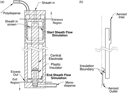
Table 1. Operation parameters of the scanning DMA.

Parameter	Notation	Value
Length (cm)	L	44.38
Inner radius (cm)	R1	0.937
Outer radius (cm)	R2	1.961
Polydisperse flow rates (LPM)	Qa	0.515
Monodisperse flow rates (LPM)	Qc	0.515
Sheath flow rates (LPM)	Qsh	2.510
Excess flow rate (LPM)	Qex	2.510
Low electrode voltage (V)	Vlow	15
High electrode voltage (V)	Vhigh	9,850
Up-scan time (s)	tramp,u	10, 20, 45, 90, 240
Down-scan time (s)	tramp,d	10, 20, 45, 90, 240
Holding time at Vlow	Tlow	20
Holding time at Vhigh	Thigh	20

The PFDMA models used in previous studies have assumed that the particles are uniformly distributed across a portion of the flow between the two electrodes. On the other hand, particles enter the classification region of the TSI long column DMA after passing through a narrow annular channel where boundary layers distort that distribution, so the velocities at which particles enter the classification region vary along the width of an entrance port in the outer electrode wall. Because of the way that the annular channel alters the spatial distribution of particles entering the DMA, we include that channel as part of an extended classification region in the simulation, as shown in Figure 1a. We start the sheath flow simulation immediately downstream of the sheath flow mesh screens that are used to uniformly distribute the flow. The simulation of the flow between the coaxial, cylindrical electrodes thus extends from the mesh to the plane of the exhaust flow exit holes, though the details of those holes are not modeled; the exhaust flow exit boundary condition is treated as an atmospheric pressure boundary condition.

In that portion of the classified-aerosol outlet downstream of the adverse-gradient region, and in the entrance region, there is no electric field to drive migration, but the complexities of the flows in both of these regions contribute to particle losses, and may introduce a distribution of delays beyond those associated with the classification region or the detector. Since the classified sample flow is discharged from the DMA through a side port, and the DMA entrance region includes an off-center inlet, the flows in these regions are simulated using the full, three-dimensional geometry.

The performance of a DMA is described by a transfer function that allows one to predict the signals produced when sampling an aerosol with a known size distribution or, alternatively, to infer the size distribution of the sampled aerosol from the signals (particle counts) in the different measurement channels. Knutson and Whitby (1975) defined the steady-state (constant-voltage) DMA transfer function, , as the probability that a particle of mobility will be transmitted through the classification region of the DMA when the DMA voltage and flows are set such that the mobility of the particle that passes from the centroid of the incoming aerosol flow to the centroid of the classified sample flow is . Hereafter, the mobility of the particle that passes from centroid to centroid will be called the “centroid mobility.” Under these conditions, and with a constant aerosol source, the value of the transfer function is simply the ratio of the flow of particles of mobility that leaves in the classified aerosol outlet flow at operating condition to that present in the incoming aerosol flow, i.e., (3) where and are the flow rates of the incoming polydisperse aerosol, and the outgoing classified aerosol sample, respectively, and and are the corresponding incoming and exiting particle number concentrations.

If we similarly define the centroid mobility for the scanning DMA, the centroid mobility continuously changes with time during the scan, i.e., , so the transfer function must be expressed in terms of time. For plug flow (uniform velocity) within the DMA, , where is the average voltage experienced by a particle that exits at time as it transits through the DMA on the centroid trajectory (Wang and Flagan 1990). Because particles are counted after leaving the DMA, the appropriate time to relate to particle mobility is the time at which the particle exits the classification region of the DMA, ; thus, we denote the centroid mobility as .

For plug flow, all successfully transmitted particles require the same time to pass through the classification region. In contrast, the nonuniform velocity that results from boundary layers within the classification region allows particles that entered the DMA at different times and, therefore, that experience different field strengths during their transit to exit the DMA at the same time.

Particles of a given mobility enter the DMA continuously at a rate ; the flow rate that may contain classified particles is Q_c. The particle concentration in the classified sample flow varies with time, i.e., . Assuming a constant source of incoming particles of mobility Z, and counting all particles of that mobility that are counted in the course of a scan, the transfer function for the scanning DMA logically becomes (4) where is the number of particles transmitted during the scan. Because the time-varying voltage allows particles of a given mobility that enter the classification region at different times to exit at the same time, the transfer function for the scanning DMA can exceed unity (Dubey and Dhaniyala 2008; Mamakos, Ntziachristos, and Samaras 2008). This added complexity requires a different approach to determination of the transfer function of the scanning DMA from that used in earlier, steady-state DMA studies.

In the present study, we do not attempt to derive a theoretical model to account for this variation; instead, we seek to capture the effects of the scan on the transfer function through Brownian dynamics simulations. To include all of the factors that affect the transfer function, we have examined a particular scanning DMA, the TSI Model 3081A long-column DMA, simulating flows and electric fields for the exact geometry of that instrument, including its entrance and exit regions, using COMSOL Multiphysics to obtain a finite-element solution of the Navier–Stokes equations for the flow field, and of Maxwell’s equations for the quasi-steady-state electric field. Brownian dynamics (Monte Carlo) simulations of particle Brownian motion were used to account for the effects of diffusion on the transmission of particles through the DMA.

We have subdivided the internal geometry of the DMA into three regions: (i) an upstream entrance region where we probe losses as the flows are brought into the classifier; (ii) the extended classification region described above; and (iii) the grounded portion of the DMA exit downstream of the adverse gradient. To elucidate the effects of the off-axis aerosol sample inlet and classified aerosol outlet ports, three-dimensional models were used to simulate the flows in the grounded portions of the entrance and exit regions. The mesh grid densities for the entrance and exit regions were set to the “extra fine” level within COMSOL. The numbers of elements in used in the simulations of the entrance (inlet) and exit (outlet) regions were each about , requiring about 12 GB of RAM in each of the COMSOL simulations. The flow and electric fields in the classification region were represented using a two-dimensional, axisymmetric model to reduce computation time, using about grid elements. The electric field and fluid motion within each of these regions were calculated once; the results are stored in a gridded format for use in the study of particle trajectories.

To place the present work in context relative to the previous, simplified, parallel-flow models of the classification region between the coaxial, cylindrical electrodes, we also represent particle transmission for fully developed laminar flow using the traditional, idealized, parallel-flow DMA model (PFDMA-L). We note that, for the flow rates considered here, the flow within the DMA rapidly approaches fully developed laminar flow, so this is a reasonable model to the extent that the PFDMA model accurately describes the DMA. Because nondiffusive particle classification during plug flow has previously been shown to attain the same transfer function as that for the constant voltage DMA (Wang and Flagan 1990), we do not simulate the plug flow limit, but, rather apply the Stolzenburg (1988) model to predictions for that idealized representation.

Once the flow and electric fields are obtained, diffusional trajectories through each of these regions are modeled using Brownian dynamics (Monte Carlo) simulations. For a small time step, the incremental change in the variance from the position that a particle would reach by advection and electrophoretic migration is given by the Einstein relation, (5) where χ denotes one of the Cartesian coordinates, x, y, or z. Within the entrance and exit regions, three-dimensional Brownian motion is simulated wherein, in a time step , the particle motion is described by (6) where is a random variable in a Gaussian distribution with standard deviation σ, and zero mean. The integral terms describe advection and electrophoretic migration; the Gaussian term accounts for Brownian motion. The entrance and exit regions use local origins, with the -coordinate along the DMA symmetric axis, as shown in Figure 1a and b. For the classification region, the axisymmetric, two-dimensional model employed here combines the Brownian contributions in the x and y directions into the r component (see Supplementary Information for illustration, Figure S4, and derivation), so that (7)

The kinematic velocity in each direction is the sum of the local fluid velocity and that due to electrophoretic migration, , which can be obtained using the flow and electric field data obtained from the finite element calculations. For the simulation within the classification region, the z-coordinate is along the DMA symmetric axis, as shown in Figure 2.

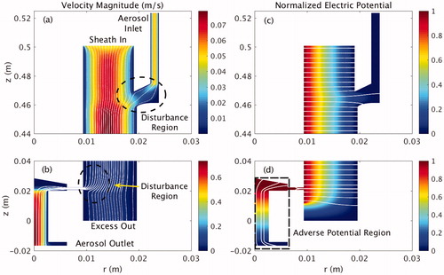
Figure 2. Magnitude of fluid flow velocity and electric potential within the classification region: (a) flow field in the upper region; (b) flow field in the lower region; (c) electric field in the upper region; (d) electric field in the lower region. Note that the color scales in (a) and (b) are different. The white lines in (a) and (b) represent the fluid flow streamlines, and those in (c) and (d) are the electric field lines. The adverse electric potential gradient region is labeled in (d).

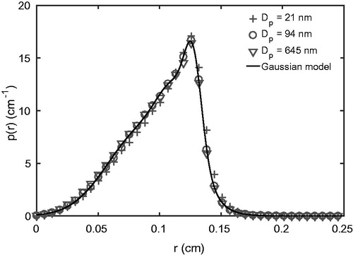
To enable coupling of the models of the classification and exit regions, the aerosol outlet boundary of the classification region is subdivided into 100 radial bins to record the exit radial distribution p(r) of the transmitted particles, which are fitted to three-term Gaussian model, i.e., (8) where a_i, b_i, and c_i are fitting coefficients. These spatial distribution fits were then used as input to simulation of the exit region. Steady-state, three-dimensional, laminar flow simulations with the COMSOL Multiphysics particle tracing module were performed for the entrance and exit regions.

Flow and electric field data from the COMSOL Multiphysics simulations were imported into Igor Pro to evaluate individual particle trajectories in the two-dimensional simulations. At each time step of the simulation, a fixed number of new particles were introduced into the classification region; they were distributed with radial position so that the number concentration in the flow was constant. The times at which particles pass through the aerosol outlet boundary were recorded, as were their entrance times.

Simulations were performed for the conditions that are used in our chamber measurements of aerosol yield; these conditions, which are summarized in Table 1, correspond to a nominal nondiffusive resolving power of , and span a particle size range of 15.3 nm nm. Scan times of s were simulated (our chamber measurements have typically been employed s) in order to explore the effect on differences between the SEMS transfer function and that of the classic, stepping mode (DMPS) operation of the DMA.

3. Results and discussion

3.1. COMSOL simulations

Figure 2 shows the results of the COMSOL simulations of the flow and electric fields within the DMA classification region for the operating conditions indicated in Table 1, focusing on the aerosol inlet and outlet regions. The fluid streamlines in the classification region and the fluid flow velocity magnitude are shown in Figure 2a and b. The entrance disturbance to the flow in the space between the electrodes is clearly seen on the right-hand-side of Figure 2a, as is the smaller disturbance near the aerosol outlet at the bottom of the main flow channel (Figure 2b). Figure 2c and d shows the electric flux lines and normalized potential. The distortion of the field near the entrance slot in the outer electrode has previously been identified as the cause of a small deviation from the predicted value of (Chen et al. 1999).

Figure 3a–c shows representative trajectories of 147 nm particles in the entrance, classification, and exit regions of the DMA, respectively; due to their low diffusivities, such large particles directly reveal the effects of voltage scanning on particle paths through the different regions of the DMA. This particular simulation considers a measurement cycle that begins with a constant low voltage for 20 s, followed by an exponential, 45 s up-scan. Since no electric field is present in that portion of the entrance shown in Figure 3a, these trajectories persist throughout the measurement cycle. The particles enter through a bent tube at the top of the instrument that discharges them into a plenum where a recirculation is induced (see Supplementary Information for the flow fields solution in the entrance and exit regions).

Figure 3. Particle trajectories within the DMA (a) entrance region, (b) exit region, (c) extended classification region for the actual DMA geometry, and (d) the idealized, parallel-flow classification region for 147 nm particles; the values of the length L, inner radius R₁, and outer radius R₂ are given in Table 1. The width of the aerosol sample incoming flow and classified sample outlet flow in the parallel-flow model are determined by the fraction of the total flow that corresponds to the corresponding limiting streamline.

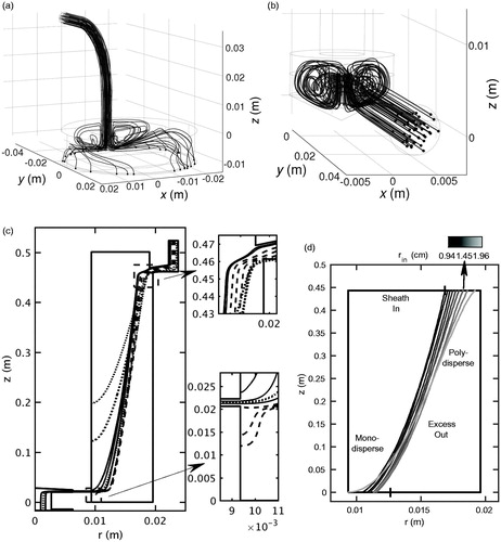
Trajectories of 147 nm particles that enter the inlet annulus at a particular instant in the measurement cycle are shown in Figure 3b. For this simulation, the particles enter the inlet annulus close to the peak in their transmission efficiency at s, where t₀ denotes the time at the start of the voltage ramp. The particle trajectories depend upon their initial radial position in the annulus. Particles that enter in the core of the flow in the annulus, dashed lines in Figure 3b, are rapidly advected through the classification region, and exit it with the excess air discharge flow. Those that enter the inlet annulus at smaller radii at this same instant of time (solid lines in Figure 3b) may be transmitted to the classified sample outlet flow. Those that enter near the outer radius of the inlet annulus (dotted lines in Figure 3b) pass through the annulus slowly due to the boundary layer, and enter the region between the electrodes when the voltage is high. As a result, they migrate quickly toward the central electrode, where they deposit. For particles in this boundary layer to be transmitted, they must enter the annulus earlier in the scan when the electric field strength is lower.

This snapshot of particles that enter the annulus at one instant of time shows that both the entrance time and the position of the particle within the aerosol inlet determine whether it can successfully penetrate through the classification region and be included in the classified sample outlet flow. Particles entering on any trajectory can be efficiently transmitted to the classified aerosol outlet flow, provided they enter the annular region at the appropriate instant of time. The transfer function must, therefore, account for all particles of a given mobility that exit the classifier at time, , regardless of their entrance times.

After passing through a downstream exit port in the central electrode, classified particles are transmitted into a cylindrical channel along the axis of that electrode; particle migration in the adverse potential gradient in this region affects their transmission efficiency (Kousaka et al. 1986). The radial distribution, shown in Figure 4, is the cumulative result for particles in a complete up-scan. The particle beam sweeps through the particle exit slot slowly at the beginning of the up-scan owing to the low electric migration velocity. Thus, the time-weighted particle penetration will be higher at  mm compared to that near the centerline (r = 0). Because the primary deposition mechanism in the adverse gradient region is electrophoretic migration, these losses are similar for particles of very different mobilities (Zhang and Flagan 1996). The radial distribution was fitted to Equation (8)(8) for use in the exit region simulations. At the bottom of the exit channel, particles enter a plenum where another recirculation zone exists, shown in Figure 3c. Ultimately, the surviving particles exit through a cylindrical port to one side at the base of the instrument.

Figure 4. Spatial distribution of particles exiting the aerosol outlet of the DMA classification region. Data are fitted with a 3-term Gaussian model, , where , and are the fitting parameters.

In contrast to the real instrument, the PFDMA-L simulation, shown in Figure 3d, distributes the incoming particles across the flow between the electrodes without distorting the velocity profile, so much less trajectory crossing takes place; that which does occur happens as the particles approach an annular sample extraction portion of the space between the electrodes in this simplistic model, which captures particle behavior only in the region between the electrodes. Those particles that enter the PFDMA-L classification region near the inner (small radius) limit of the sample flow, e.g., mm, where the fluid velocity is high, experience relatively short residence times compared with those that enter on the corresponding streamlines of the real DMA where the boundary layer in the inlet annulus slows the flow.

3.2. Scanning DMA transfer function for low diffusivity particles

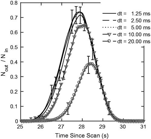
Simulations of the entrance, classification, and exit regions of the DMA operated under the conditions indicated in Table 1 were performed for 52 logarithmically spaced electrical mobilities ranging from ( nm) to ( nm). Particles of each size were introduced into the classifier at a constant rate of 200 particles per time step throughout the scan. The transfer functions were obtained by locally weighted scatterplot smoothing (LOESS; Cleveland 1979) of the raw data using second order polynomials. The error bars show the root-mean-square sum of residuals of the raw data from this fitted function.

Accurate estimation of the transfer function using Brownian dynamics simulation requires a short time step, but the computational cost increases dramatically with decreasing step size. The approach of an asymptotic form for the transfer function was explored by performing simulations with time steps, , ranging from 1.25 to 20 ms. The resulting ratio of the flow of particles contained in the classified aerosol outlet flow (number/s) to the entering particle flow rate is shown as a function of time-in-scan in Figure 5. Decreasing the time step from 20 to 10 ms increased the peak transmission two-fold; the peak value approaches an asymptotic limit as approaches 1.25 ms for small, high-diffusivity, 24.5 nm particles. Long time steps increase the likelihood that, during a single time step, simulated diffusional motion will bring a particle to a flow boundary, particularly during the low voltage portion of the particle’s transit through the classification region when particles are advected close to, and nearly parallel to an electrode surface, i.e., the outer electrode in the up-scan, and the inner electrode in the down-scan. Shorter time steps make it possible to better track the particle trajectories through this critical portion of their time in the classification region, and, therefore, yield higher transmission probabilities. As particle size increases, diffusivity and σ_r decrease, enabling longer time steps. With time step of 1.25 or 2.5 ms, the total number of transmitted particles in the simulated scans were and .

Figure 5. Scanning transfer functions for 24.5 nm particles through the real DMA geometry as determined using the indicated simulation time steps based for a ramp time of s.

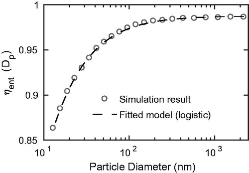
The steady-state, three-dimensional simulation of flow in the entrance region produced the penetration efficiency as a function of the mobility-equivalent diameter shown in Figure 6. For these operating conditions, diffusional losses become significant as particle diameter decreases below about 70 nm, though transmission was high, even for the smallest particles.

Figure 6. Penetration efficiency through the DMA entrance region as a function of particle diameter for an aerosol flow rate of LPM.

That portion of the exit within the central electrode extending through and the downstream insulator have been included in the classification region in order to account for the adverse potential gradient, so its effects are part of the classification region transfer function reported here. While steady-state can be assumed for the region upstream of the entrance annulus, the distribution of delay times during passage through the exit region can distribute the particles into different counting bins. Therefore, the exit region analysis considers the time-dependent penetration through the exhaust plenum, where the strong recirculation seen in Figure 3c occurs, and the lateral exit tube. The efficiency of particle penetration through this region is shown as a function of particle size in Figure 7a. The overall penetration efficiency within the exit region is close to unity, ranging from 96 to 99.5% as shown in Figure 7b; penetration decreases with decreasing size due to diffusion. The mean residence time within this region for those particles that are transmitted through it, shown in Figure 7c, ranges from 0.20 to 0.22 s, and increases with particle size because diffusion reduces the concentrations of the smallest particles in the boundary layer where velocities are low. While these times are short compared to that in the classifier for the low flows considered in this study, they could become important in measurements of smaller particles.

Figure 7. (a) Penetration distribution through the DMA exit region as a function of particle diameter and elapsed time; (b) the time variation of the penetration for 13, 34, and 2,204 nm particles; (c) cumulative particle penetration efficiency as a function of particle diameter; (d) mean residence time through the DMA exit region as a function of particle diameter.

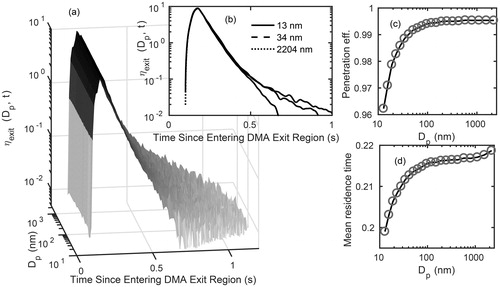
The data from the simulations shown in Figure 7a reveal two sources of uncertainty in the particle trajectories that affect the transmission through the exit region as a function of time. These uncertainties also affect all of the simulations described in this article. First is the uncertainty that arises as Brownian diffusion causes small particles to deviate from the kinematic trajectories that nondiffusive particles of the same size would follow. Because the diffusivity increases with decreasing particle size, this “true uncertainty” is most pronounced for small particles. Hence, we shall explore the behavior of large, low diffusivity (e.g., 147 nm ones) at several points throughout this article to minimize this source of and, thereby, to elucidate the direct effects of scanning on the SEMS/SMPS response. With regard to the efficiency of transmission of particles through the exit region of the DMA, the data in Figure 7a show that large particles continue to be transmitted long after the transmission of small particles has ceased. The large particles follow trajectories determined by a balance between aerodynamic forces, while the small particles diffuse away from those kinematic trajectories, allowing some of them to reach the walls where they deposit. The second source of uncertainty is inherent to Brownian dynamics simulations owing to the finite number of particle trajectories that can be simulated in any reasonable computational time. If the true number of particles that should be counted in a given time interval is , the statistical uncertainty in the number actually detected is according to Poisson statistics. In Figure 7a, the transmission probability looks smooth when the efficiency is high since many particles are counted, but fluctuations become a significant part of the signal where the efficiency is lower, and fewer particles are counted. The uncertainty resulting from diffusion is real, while the statistical uncertainty results from simulating a limited number of particle trajectories. Additional computational uncertainties arise due to compromises made in the grid density and time steps employed in this exploratory study. Nonetheless, the simulations reveal features in SEMS/SMPS performance that have previously escaped attention.

To determine the scanning DMA transfer function, the entrance and exit times of each particle that is successfully transmitted are stored. Because the clearest indication of the effect of scan time on the DMA transfer function is found in simulations of large, low diffusivity particles, we first consider relatively large ones.

The entrance times of successfully transmitted 147 nm particles for a 45 s up-scan exhibit a highly skewed distribution, and differ dramatically between the geometric model (G-DMA) and the idealized, laminar and parallel flow model (PFDMA-L), as seen in Figure 8a. The long tail toward the small entrance-time limit of the distribution results from particles that enter near the wall, where the velocity is low. Particles that enter where the velocity is high have quite uniform transit times, so there is no tail for late entering particles. This distortion of the entrance time distribution in the geometric model of the real DMA results from the two boundary layers in the entrance annulus, while particles entering the PFDMA-L model experience only a single boundary layer region. While the entrance time distribution of 147 nm particles during down-scan operation in the G-DMA model shows tails toward late exit times, the entrance-time distribution of the PFDMA-L model is close to triangular shape (Figure 8b).

Figure 8. Temporal distributions of entrance and exit times for singly charged 147 nm particles that are successfully transmitted through the DMA classification region for the geometric-DMA (G-DMA) model, or through the classification region of the parallel-laminar-flow (PFDMA-L) model. Ramp times for both upscan (a) and downscan (b) was  = 45 s ( = 6.94 s). The voltage was held constant for 20 s before the start of each scan (up or down).

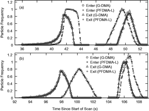
In contrast to the entrance time distribution, the exit time distribution for the up-scan approaches the triangular, nondiffusive form seen for large particles in the constant-voltage DMA. As defined in Equation (3)(3) , the scanning DMA transfer function describes the temporal distribution of particles exiting the classification region. Both G-DMA and PFDMA-L models show skewed exit time distributions for the down-scan operation.

Since the exit time determines into which time bin a particle is counted, the up-scan yields better behaved data than does the down-scan, a conclusion that many users have drawn from scanning DMA data. Since this corresponds most closely to the time bins into which counts are accumulated during measurements, further discussion of the results of this study will focus on the exit times.

In the limit of long scan times (large ), the voltage changes little during any particle’s transit through the classification region. Hence, we intuitively expect the transfer function to asymptotically approach that of the constant voltage DMA. As suggested by Wang and Flagan (1990), the nondiffusive transfer function preserves its triangular form for plug flow. We see in Figure 9 that, even with the pronounced boundary layers produced by laminar flow in real DMAs, the triangular form is preserved for a wide range of scan times. On the other hand, as decreases, the shape of the transfer function becomes increasingly distorted for both fully developed laminar flow (PFDMA-L) and the real-world flow patterns of the G-DMA. Some of the particles are artificially introduced into the high-velocity region of the flow in the PFDMA-L, so the mean residence time in that model is artificially low. In contrast, a fraction of particles in a real scanning DMA (and in the G-DMA model) must pass through the boundary layer region where the velocity is low, increasing the mean residence time slightly over that of the plug flow. The laminar and plug-flow PFDMA models exclude diffusional losses in the entrance annulus, and electrophoretic particle losses in the adverse gradient region, so the transmission probabilities estimated by both models are higher than predicted using the real DMA geometry. Indeed, the apparent transmission efficiency in the idealized laminar PFDMA can significantly exceed unity (as much as 25%) during fast scans (–20 s) because the particles entering late in the scan can catch up with those that entered earlier.

Figure 9. Up-scan transfer functions for 147 nm particles with a ramp time of , 20, 45, 90, and 240 s (corresponding to , 3.08, 6.94, 13.9, and 37.0 s) for the geometric-DMA (G-DMA), parallel-laminar-flow (PFDMA-L) and parallel-plug-flow (PFDMA-P) models as a function of the classifier exit time. The static-DMA model uses the constant-voltage transfer function, as in the PFDMA-P model, but evaluates the transfer function at the time at which particles exit the DMA.

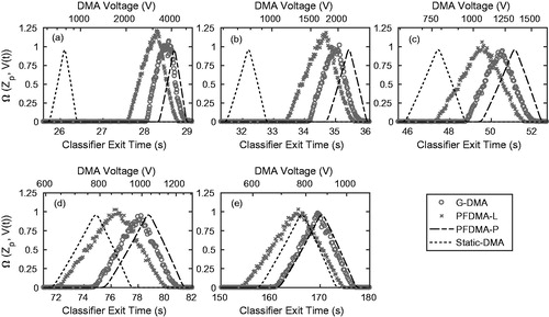
A natural misinterpretation of the scanning-mode data is to evaluate the transfer function at the voltage at the time when particles exit the DMA, usually under the assumption of uniform velocity. In essence, this amounts to treating the scanning-mode data as though it resulted from operation of the DMA with the voltage held constant at that value. Thus, for an up-scan (Figure 9), this “static” transfer function suggests that the particles are classified at the highest voltage that they experience during their transit through the classification region, i.e., that at the time when they exit the classification region. For a given mobility, this model would require that a particle would, in this static model exit at a lower voltage than it actually would during scanning operation; this corresponds to an earlier predicted exit time than in practice. Similarly, for a down-scan, the particle would be predicted to exit at a higher voltage than in reality, again leading to an early estimated exit time. The particle size inferred from a particle that is observed to exit the voltage-scanned DMA would, therefore be substantially larger than reality for an up-scan, and smaller for a down-scan. The apparent bias is exacerbated by plumbing delays between the exit to the DMA and the detection point within the CPC. The observed counts to the scanning-DMA voltage at any instant of time will likely lead to erroneous estimations of particle size, and should be avoided. Instead, one must invert the data using the best estimate of the instrument response function, taking into account both the SEMS/SMPS transfer function and the additional delays that occur downstream of the DMA.

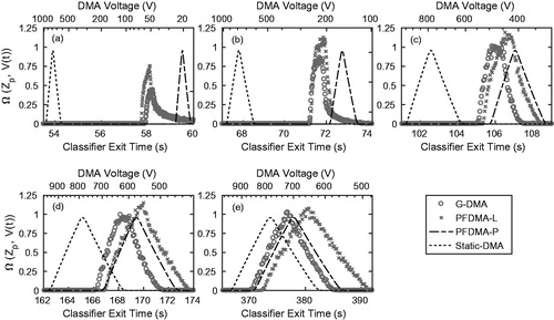
The effects of ramp time on down-scan transfer functions for the three models are shown in Figure 10; the down-scan transfer function for short scan times is highly skewed to long exit times. The extent to which the down-scan transfer function exceeds unity at short scan times is lower than that for up-scans, while the tail toward small mobilities (late exit time) increases in length. During the down-scan, particles initially migrate quickly across the classification region, but their radial migration then slows, and particles spend much of their transit time in the low velocity near the inner electrode, delaying their passage through the classification region. Increasing the scan rate increases this boundary layer effect. In contrast to the up-scan, only very slow down-scans yield transfer functions that approach the triangular form of the constant-voltage DMA.

Figure 10. Down-scan transfer functions for 147 nm particles with ramping time  = 10, 20, 45, 90, and 240 s (corresponding to  = 1.54, 3.08, 6.94, 13.87, and 37.00 s) for the geometric-DMA (G-DMA), parallel-laminar-flow (PFDMA-L), parallel-plug-flow (PFDMA-P), and static DMA models.

3.3. Instantaneous classification transfer function over the full range of particle sizes

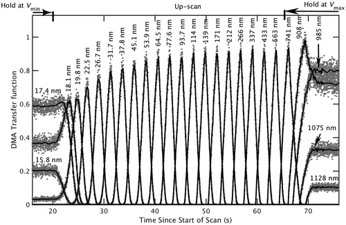
To enable application of the simulated transfer function of the classification region to SEMS/SMPS data inversion, G-DMA simulations were performed for electrical-mobility-equivalent particle diameters ranging from 15.3 to 1,130 nm in a 45 s up-scan, yielding the transfer functions shown in Figure 11. The scattered dots representing the raw data from the simulation, while the curves show the LOESS-smoothed results. One would expect the transfer functions to be smooth functions of time; the scatter in the simulation data result from the Brownian dynamics simulations owing to the limited number of particles simulated. Particles between 15.3 and 19.8 nm diameter can penetrate the classification region in the first 20 s of the scan, when the voltage of the electrode is held at . The transmission efficiencies of these particles remain unchanged until the voltage ramp begins, yielding a constant transfer function during this period; a similar plateau in the transmission efficiencies for large particles (800–1,130 nm) starts at s, 6 s after the voltage reaches and is, therefore, held constant. This time is somewhat shorter than the mean fluid residence time of 8.21 s due to rapid passage of the particles through the boundary layers of the classification region.

Figure 11. Scanning DMA transfer functions for singly charged particles, with electric mobility equivalent diameters ranging from 15.8 to 1130 nm. Scattered dots represent the raw data from the simulations, while the solid lines are the result obtained by applying locally weighted scatterplot smoothing (LOESS) to the raw data.

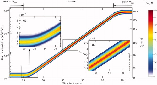
The variation of the transfer function with time-in-scan and mobility is shown in Figure 12; the continuous plot was created by interpolating the transfer functions in Figure 11 over the full range of the particle sizes. The insets show the transmission efficiency at the transition from the low-voltage holding period to the voltage ramp (a), and that during the ramp (b). Because of diffusional losses, the overall transmission efficiency when the voltage is held at is relatively low, and the transfer function is broad. Note that the electrical mobility scale is reversed so that the smallest particles appear at the bottom of the plot.

Figure 12. The scanning DMA transfer function as a function of the time-in-scan and the inverse particle electrical mobility. The inset (a) shows the transfer function during the transition from the low-voltage holding period to the ramp, while inset (b) shows the transfer function for particles whose transit is fully within the ramp.

3.4. Instantaneous transfer function of the integrated scanning DMA

Thus far, we have only characterized the instantaneous classification transfer function, Equation (3)(3) . The instantaneous transfer function of an actual scanning DMA must also account for particles losses in the entrance, and exit regions, as well as any delays in the classification (from its entrance to its exit) and the exit regions, i.e., (9) where and are the penetration efficiencies of the entrance and exit regions that were shown in Figures 6 and 7, and denotes the convolution operator, .

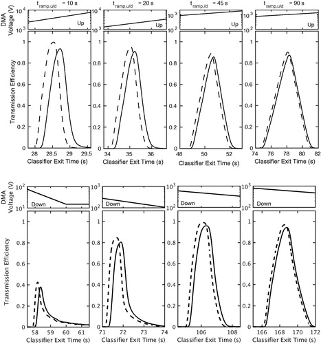
Figure 13 shows the instantaneous transfer functions of the integrated scanning DMA for 147 nm particles, i.e., large, nondiffusive ones, with scan times ranging from 10 to 90 s for both up-scan and down-scan operations. The difference between the transfer function of the integrated DMA and that of the classification region alone can be attributed to the combined effects of distribution of particle residence times within the exit region that distorts the shape of the transfer function and particle losses in both regions.

Figure 13. Transfer functions of the classification region (dashed line) and that of the complete DMA (including entrance and exit regions, solid line) for up-scan (upper panel) and down-scan (lower panel) operation for  = 10, 20, 45, 90 s (corresponding to  = 1.54, 3.08, 6.94, 13.87 s).

4. Conclusions

This study has examined the transfer function of a real DMA when operated in as part of a SEMS or SMPS. Detailed finite-element simulations of the flows and electric fields in the DMA are combined with Brownian dynamics (Monte Carlo) simulations to determine the transfer function for diffusing particles during voltage scanning. These numerical simulations reveal important differences from the idealized parallel-flow/perpendicular-electric-field models of the DMA that have been considered in most previous transfer function predictions. The effects of these differences are often small when the DMA is operated at constant voltage, but can lead to profound changes in the transfer function when operated in scanning mode, particularly for fast scans.

The present study has focused on a single instrument, the TSI Model 3081 long-column DMA, operated at flows that allow the instrument to probe relatively large particles. While the details will differ if the operating conditions are changed, or if a different classifier is used, the results of this study raise important questions about the interpretation of scanning DMA measurements. The elegant Stolzenburg transfer function (Stolzenburg 1988) may closely approximate the instantaneous transfer function for sufficiently slow, increasing-voltage scans in a cylindrical DMA, but fails to describe the instrument when scans are fast. Further study will be needed to generalize these results to other DMAs or operating conditions.

To simulate scanning mobility particle classification, both that part of the entrance region of the DMA that influences the distribution of particles across the aerosol sample entrance into the region between the electrodes, and the region where particles pass through an adverse potential gradient in the DMA exit were included as part of an extended classification region. The value of the classification transfer function for particles of a given mobility at exit time accounts for the contributions of incoming particle that entered the DMA at all earlier times; because particles at different locations within the incoming aerosol sample experience different transit times, its value may exceed unity during fast scans. For an exponentially increasing voltage ramp (up-scan), the transfer function for nondiffusive particles is triangular in form for all but the fastest ramps, i.e., smallest . In contrast, the down-scan exhibits a long tail at long time-in-scan, and yields a seriously distorted transfer function shape for all but the slowest scans. This difference in transfer function forms validates the common approach of basing scanning-DMA measurements on the up-scan, although, when the full transfer function is known, even down-scan data can be inverted to obtain the particle size distribution.

This article has focused on obtaining the instantaneous transfer function of the DMA, and has not considered distortions of the measurements due to finite detector time response or other factors outside of the DMA. Early observations of asymmetry between up-scans and down-scans identified the slow response of the CPC used in those studies as the key factor leading to distortion in SEMS/SMPS instrument response (Russell, Flagan, and Seinfeld 1995), though the DMA transit time distribution was later shown to be an issue (Collins et al. 2004; Mamakos, Ntziachristos, and Samaras 2008; Dubey and Dhaniyala 2008). Only the latter effects (those within the DMA) have been treated here, with the added features of particle diffusion and real DMA geometry.

While we have shown that the distortions caused by scanning the DMA voltage are more complex than previously described, SEMS/SMPS data inversion must also consider distortions due to plumbing downstream of the DMA, as well as the response-time-distribution of the detector. Therefore, data inversion requires yet another transfer function, that for the integrated SEMS/SMPS instrument that includes the effects of the DMA, downstream plumbing, and the particle detector, typically a CPC. In addition, the full SEMS/SMPS integrated instrument transfer function must account for the finite time period over which particles are counted for each time channel. This integrated transfer function for the full instrument is the topic of the companion to this article (Mai et al. 2018).

The present work on the scanning DMA transfer function has explored the transfer function for a limited range of conditions for one SMPS system. Ultimately, the scanning DMA transfer function is needed for every combination of flow rates, scan profiles, DMA column and, as addressed in the companion paper, CPC that is used in aerosol measurements. This article demonstrates the need for detailed understanding of the interplay between the flows and the time-varying electric field within the DMA during a SEMS/SMPS measurement. Details that have little effect in stepping-mode (DMPS) operation of the DMA become important in the unsteady scanning-mode measurements if they make the transit times for particles dependent upon the time in the scan when particles enter the classification region. Owing to the computational demands of this exploratory study, neither the computational grid nor the time step were fully optimized, so there remains room for improvement in both the finite element flow and electric field calculations and in the Brownian dynamics simulations. However, as will be shown in Paper II (Mai et al. 2018), the transfer function derived in this article enables accurate inversion of SEMS data during rapid scans, both the commonly used, increasing voltage scan and decreasing voltage scans that lead to greater apparent distortions in the data. Given the number of DMA designs in use today, and the range of operating conditions used for each of those instruments (flow rates, voltage limits, scan rates, etc.), more efficient approaches to transfer function determination are needed to enable the SEMS/SMPS user community to properly analyze their data. If one must use the constant-voltage transfer function in lieu of one determined for the DMA operated under scanning conditions, the characteristic scan time, , should be large, i.e., much greater than the mean residence time in the classification region of the DMA.

Acknowledgments

The authors thank Dr. K. Beau Farmer of TSI Inc. for providing detailed design drawings of the TSI Model 3081A DMA that made it possible to simulate flows, fields, and particle trajectories in the real instrument. We thank Yuanlong Huang, Wilton Mui, Amanda Grantz, Johannes Leppä, Paula Popescu, and John Seinfeld for useful discussions.

Additional information

Funding

This work was supported by the National Science Foundation under Grant No. AGS-1602086.

References

- Attoui, M., and J. F. de la Mora. 2016. Flow driven transmission of charged particles against an axial field in antistatic tubes at the sample outlet of a differential mobility analyzer. J. Aerosol Sci. 100:91–96. doi:10.1016/j.jaerosci.2016.06.002.
- Chen, D.-R., and D. Y. Pui. 1997. Numerical modeling of the performance of differential mobility analyzers for nanometer aerosol measurements. J. Aerosol Sci. 28(6):985–1004. doi:10.1016/S0021-8502(97)00004-9.
- Chen, D.-R., D. Y. Pui, D. Hummes, H. Fissan, F. Quant, and G. Sem. 1998. Design and evaluation of a nanometer aerosol differential mobility analyzer (nano-DMA). J. Aerosol Sci. 29:497–509. doi:10.1016/S0021-8502(97)10018-0.
- Chen, D.-R., D. Y. H. Pui, G. W. Mulholland, and M. Fernandez. 1999. Design and testing of an aerosol/sheath inlet for high resolution measurements with a DMA. J. Aerosol Sci. 30(8):983–99. doi:10.1016/S0021-8502(98)00767-8.
- Cleveland, W. S. 1979. Robust locally weighted regression and smoothing scatterplots. J. Am. Stat. Assoc. 74(368):829–36. doi:10.2307/2286407.
- Collins, D. R., D. R. Cocker, R. C. Flagan, and J. H. Seinfeld. 2004. The scanning DMA transfer function. Aerosol Sci. Technol. 38(8):833–50. doi:10.1080/027868290503082.
- Collins, D. R., R. C. Flagan, and J. H. Seinfeld. 2002. Improved inversion of scanning DMA data. Aerosol Sci. Technol. 36(1):1–9. doi:10.1080/027868202753339032.
- Dubey, P., and S. Dhaniyala. 2008. Analysis of scanning DMA transfer functions. Aerosol Sci. Technol. 42(7):544–55. doi:10.1080/02786820802220258.
- Dubey, P., and S. Dhaniyala. 2011. A new approach to calculate diffusional transfer functions of scanning DMAs. Aerosol Sci. Technol. 45(8):1031–40. doi:10.1080/02786826.2011.579644.
- Fissan, H., C. Helsper, and H. Thielen. 1983. Determination of particle size distributions by means of an electrostatic classifier. J. Aerosol Sci. 14(3):354–7. doi:10.1016/0021-8502(83)90133-7.
- Flagan, R. 1999. On differential mobility analyzer resolution. Aerosol Sci. Technol. 30(6):556–70. doi:10.1080/027868299304417.
- Franchin, A., A. Downard, J. Kangasluoma, T. Nieminen, K. Lehtipalo, G. Steiner, H. E. Manninen, T. Petaja, R. C. Flagan, and M. Kulmala. 2016. A new high-transmission inlet for the Caltech nano-RDMA for size distribution measurements of sub-3 nm ions at ambient concentrations. Atmos. Meas. Tech. 9(6):2709–20. doi:10.5194/amt-9-2709-2016.
- Knutson, E. O., and K. T. Whitby. 1975. Aerosol classification by electric mobility: Apparatus, theory, and applications. J. Aerosol Sci. 6(6):443–51. doi:10.1016/0021-8502(75)90060-9.
- Kousaka, Y., K. Okuyama, M. Adachi, and T. Mimura. 1986. Effect of Brownian diffusion on electrical classification of ultrafine aerosol particles in differential mobility analyzer. J. Chem. Eng. Jpn. 19(5):401–7. doi:10.1252/jcej.19.401.
- Mai, H., W. Kong, J. H. Seinfeld, and R. C. Flagan. 2018. Scanning DMA data analysis II. Integrated DMA-CPC instrument response and data inversion. Aerosol Sci. Technol. doi:10.1080/02786826.2018.1528006.
- Mamakos, A., L. Ntziachristos, and Z. Samaras. 2008. Differential mobility analyser transfer functions in scanning mode. J. Aerosol Sci. 39(3):227–43. doi:10.1016/j.jaerosci.2007.11.005.
- Mui, W., H. Mai, A. J. Downard, J. H. Seinfeld, and R. C. Flagan. 2017. Design, simulation, and characterization of a radial opposed migration ion and aerosol classifier (ROMIAC). Aerosol Sci. Technol. 51(7):801–23. doi:10.1080/02786826.2017.1315046.
- Russell, L. M., R. C. Flagan, and J. H. Seinfeld. 1995. Asymmetric instrument response resulting from mixing effects in accelerated DMA-CPC measurements. Aerosol Sci. Technol. 23(4):491–509. doi:10.1080/02786829508965332.
- Stolzenburg, M. R. 1988. An ultrafine aerosol size distribution measuring system. PhD thesis, Univ. Minnesota.
- Tammet, H. 2015. Passage of charged particles through segmented axial-field tubes. Aerosol Sci. Technol. 49(4):220–8. doi:10.1080/02786826.2015.1018986.
- Ten Brink, H., A. Plomp, H. Spoelstra, and J. Van De Vate. 1983. A high-resolution electrical mobility aerosol spectrometer (MAS). J. Aerosol Sci. 14(5):589–97. doi:10.1016/0021-8502(83)90136-2.
- Wang, S. C., and R. C. Flagan. 1990. Scanning electrical mobility spectrometer. Aerosol Sci. Technol. 13(2):230–40. doi:10.1080/02786829008959441.
- Zhang, S.-H., and R. C. Flagan. 1996. Resolution of the radial differential mobility analyzer for ultrafine particles. J. Aerosol Sci. 27(8):1179–200. doi:10.1016/0021-8502(96)00036-5.