A language to simplify computation of differential mobility analyzer response functions

Abstract

A language for computation of differential mobility analyzer (DMA) response functions is introduced. The language consists of short programming language expressions that evaluate to the size distribution of particles exiting a DMA. The language permits application of the same framework to single and tandem DMA setups. Expressions are derived for calculation of the convolution matrix used in inversion of size distribution data, calculation of the convolution matrix for transit through tandem DMA systems, and calculation of the size and mobility distribution through DMA systems that involve one or multiple DMAs. The contribution of multiply charged particles to the total response distributions can be explicitly resolved. The derived convolution matrix is suitable for inverting scanning mobility particle sizer response functions using standard regularization techniques. Users can modify and substitute any of the convolution terms—comprising the DMA transfer function, detector efficiency, loss rate, and charging efficiencies—to express response functions of nonstandard DMA configurations. Example applications are presented, including classification of particle size, measurement of size-resolved cloud condensation nuclei activity, characterization of hygroscopicity and volatility tandem DMA response functions, and characterization of the dual tandem DMA system for dimer preparation. The source code and examples are shared as free software and are hosted on an online collaborative software development platform that allows for version tracking and crediting contributors. Adoption of the language may facilitate the design and optimization of custom-built systems that involve unique arrangements of DMAs and detectors.

Copyright © 2018 The Author(s). Published with license by Taylor & Francis Group, LLC.

Editor:

• Kihong Park

1. Introduction

Manipulation of particles through electrical fields is a long-established technique (Flagan 1998). Differential mobility analyzers (DMAs) matured through several contributions in the 1950s–70s (Hewitt 1957; Knutson and Whitby 1975; Langer, Pierrard, and Yamate 1964; Liu and Pui 1974), and subsequently became widespread. The cylindrical DMA passes a polydisperse aerosol flow through an annulus gap. An electric potential is applied between the inner and outer column. The electric potential drags charged particles through a sheath flow. Particles within a narrow electrical mobility band are steered to a sample slit. All other particles exit with the excess flow.

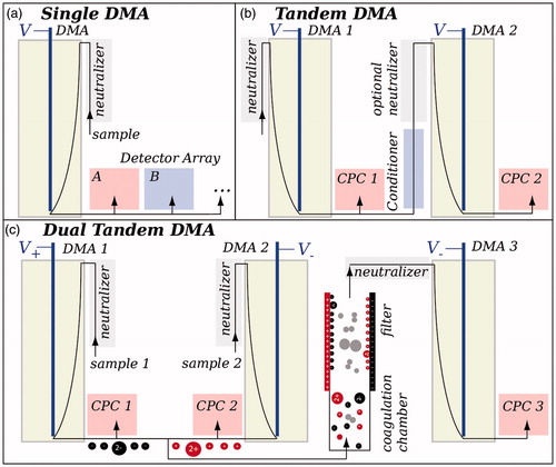
DMAs are attractive because the selected aerosol size can be predicted from first principles and depends only on the electric field strength, the Stokes drag force on the particle, number of elementary charges on the particle, and the laminar flow velocity profile of the carrier fluid. The technique is applicable over a wide span of particle sizes ranging from 1 nm to 1 µm. Size changes on the order of a single monolayer can be resolved with tandem DMA setups (Rader and McMurry 1986). DMAs are highly versatile. Park et al. (2008) reviewed an extensive set of DMA-detector configurations. Setups involving one or multiple DMAs can support several experimental designs (Figure 1). Single DMA setups are used for working with classified particles or measuring size distributions (Figure 1a). One application is the calibration of detection efficiency of an instrument. Another set of applications is to exploit differences between detectors to determine aerosol physical properties, such as refractive index, density, cloud condensation nucleation, or ice nucleation efficiency. A third application is the measurement of the particle number size distribution in scanning mode (Wang and Flagan 1990). In tandem DMA setups (Figure 1b), the first DMA is used as a classifier. The sample flow is then conditioned to induce a size change and the resulting size distribution is measured using a second DMA with a condensation particle counter (CPC) or other instrument as detector. Dual tandem DMA setups can be used to synthesize and isolate particle dimers that form via coagulation (Maisels et al. 2000; Rothfuss and Petters 2016, Figure 1c). Two DMAs are used to size select monodisperse particles of opposite charge. The two sample flows merge and particles coagulate. Coagulated charge-neutral dimers are retained during passage through an electrostatic filter. The size distribution of the dimers is measured using a third DMA.

Figure 1. Schematic of typical configurations. (a) Single DMA setups for working with classified particles and measuring size distributions, (b) tandem DMA setups for measuring aerosol volatility or hygroscopicity, and (c) dual tandem DMA setup for generating dimers via coagulation.

1.1. Problem statement

The probability that a particle of a given size exits the classifier via the sample flow is described by a DMA transfer function. Transfer functions have been described for different DMA geometries (Knutson and Whitby 1975; Zhang et al. 1995), continuously scanning DMAs (Collins et al. 2004; Wang and Flagan 1990), and tandem DMAs (Rader and McMurry 1986; Stolzenburg and McMurry 2008), including for conditions where diffusional broadening cannot be neglected (Hagwood 1999; Stolzenburg and McMurry 2008). In the absence of diffusional broadening, the nondimensional transfer function is triangular and its width is determined by the sheath-to-sample flow ratio. For fixed voltage and sheath flow, the DMA selects particles with centroid mobility z^s (z-star). Particle mobility is proportional to the charge-to-diameter ratio. Particle charge is statistically distributed and charge equilibrium is created by the upstream neutralizer. Therefore, the DMA transmits a mixture of singly and multiply charged particles of different sizes. Some particles may be lost in transit or detected with less than unit efficiency. Consequently, the measured signal is the convolution of the DMA transfer function, charging probabilities, loss rates, and detection efficiencies. The challenge of working with DMA data is to relate the measured detector response to the unknown aerosol concentration and size distribution.

The DMA response function is computed using a Fredholm integral equation of the first kind (Kandlikar and Ramachandran 1999; Stolzenburg and McMurry 2008; Twomey 1963). The equation can be discretized into a system of equations and recast in matrix form such that (1) where R is the response vector measured by the detector, N is a vector of true number concentrations, ϵ is a vector of measurement errors, and A is a matrix that subsumes the convolution terms. Equation (1)(1) can in principle be used to find the size distribution from a measured DMA response function via . This method is suitable if the Fredholm integral is approximated (e.g., Pfeifer et al. 2014). Without approximations measurement noise and rounding errors dominate the inversion, thus necessitating regularization (Hansen 2000; Kandlikar and Ramachandran 1999; Talukdar and Swihart 2003; Twomey 1963). The matrix approach is highly attractive due to its apparent simplicity in relating the size distribution and DMA response function.

The matrix approach has limitations. Writing computer code that constructs the convolution matrix is time consuming and not straightforward. For size distribution measurement, commercial systems include inversion codes that can be used. In general, however, these codes are proprietary and closed source. The algorithms used to compute the inversion are neither traceable nor modifiable for use with DMA configurations and detectors that are not supported by the manufacturer. Non-commercial inversion codes exist. Wiedensohler et al. (2012) reference 12 codes for size distribution inversion. Few of these codes appear to be documented or freely accessible.

In approximate inversions, variations in charging efficiency and size distribution across the width of the DMA transfer function are assumed negligible (e.g., Alofs and Balakumar 1982; Stolzenburg and McMurry 2008, 2018). This approximation cannot be applied to tandem DMA response functions and more specialized approaches are used (Gysel, McFiggans, and Coe 2009; Stolzenburg and McMurry 1988; Stratmann et al. 1997). Furthermore, in the mapping from N to R, the contributions of multiply charged particles to the response concentration are inaccessible. Consequently, the relative fractions of singly and multiply charged particles comprising the response concentration in each channel are unknown. However, many applications require an explicit understanding of the number and size of multiply charged particles to interpret the response function. For example, consider a size selecting DMA that is coupled with an ice nucleation instrument as detector to measure the influence of particle size on ice nucleation ability (e.g., DeMott et al. 2009). The signal is proportional to surface area for heterogeneous and volume for homogeneous freezing nucleation. To obtain the surface area or volume selected by the classifier, including contributions from multiply charged particles, the Fredholm integral must be solved. Or consider a volatility tandem DMA setup. Size classified particles are passed through an evaporation section and the resulting size distribution is measured (Bilde et al. 2003; Wright et al. 2016). Evaporation rate is proportional to surface area which leads to differential evaporation of singly and multiply charged particles. Knowledge of the charge-resolved size distribution is needed to properly interpret the tandem DMA response function.

1.2. This work

I describe a new language for modeling DMA response functions with arbitrary arrangements of DMAs. The Julia DMA language (JDL) consists of a representation of aerosol size distributions, operators to construct expressions, and functions to evaluate the expressions. It is written in the Julia language (Bezanson et al. 2017). In JDL single line computational expressions evaluate to the size distributions after passage through the DMA, obviating the need for users to implement algorithms to solve the Fredholm integral equation numerically. The convolution matrix is found via such an expression. Application of JDL is demonstrated by formulating expressions for response functions involving the three configurations shown in Figure 1, including single mobility classification, size and CCN distribution inversion, hygroscopicity and volatility tandem DMA setups with and without a second charge neutralization step, and dimer synthesis using dual tandem DMA. Response functions for the first four applications have been reported in various places before, but response functions for the dual tandem DMA setup have not yet been investigated theoretically.

The software package Differential Mobility Analyzers.jl serves as supplement to this work. Differential Mobility Analyzers contains the JDL source code and 12 Jupyter notebooks. Jupyter notebooks are a web-based application that allows blending computer code and documentation in the form of embedded figures, text, and equations. The notebooks can be accessed in viewer mode, which displays text, code, and interactive Javascript graphics. The Javascript graphics allow readers to hover over a graph to extract values from the series, to remove selected series by clicking on the legend, and to reshape the figure in a web-based application with no coding required. When opened in regular mode, the computer code can be executed in a step-by-step fashion. Nonprogramming experts can interact with the code by modifying input parameters. The supplementary notebooks also contain documentation, explanations, equations, code validation, proofs, and interactive versions of the figures presented below.

2. Methods

2.1. Definitions of particle diameter

Operation principles of the DMA are reviewed in detail in Notebook S1. The relationship between mobility and mobility diameter is (2) where k is the number of charges on the particle, e is the elementary charge, c_c is the Cunningham slip flow correction factor, η is the fluid viscosity, Z is the mobility, and D is the mobility diameter. Further, is the mobility diameter array corresponding to mobility array Z assuming that the particle carries k charges. Here, the “apparent +1 mobility diameter” is defined as (later also denoted as ) where Z is the mobility grid scanned by the DMA. The apparent +1 mobility diameter represents the diameter axis of the DMA response function. It is strictly defined via Equation (2)(2) , is an equivalent measure of mobility, and functions as an intuitive representation of the nominal mobility diameter selected by the DMA. The apparent +1 mobility diameter is ambiguous. Larger particles carrying more than one charge may have the same apparent +1 mobility diameter than smaller particles carrying fewer charges. In contrast, the mobility diameter correctly accounts for the number of charges on the particle. Note that nonspherical particles have a well-defined mobility even though they do not have a true diameter and for sub 3 nm particles the mobility diameter is not equal to the geometric diameter even for spherical particles (Larriba et al. 2011).

2.2. Fredholm integral

The discretized version of the Fredholm integral is (3) where are indices of the observed instrument channel, are indices of the physical size bins, are indices of charges carried by the particle, R_i is the instrument response in the ith bin, Z_j is the electrical mobility in the jth bin is the charge normalized centroid mobility in the ith channel, Ω is the DMA transfer function, T_c is the charging probability, T_l is the transmission loss, is the diameter of singly charged particles corresponding to mobility Z_j, is the number concentration of particles in the jth bin. The terms in the inner sum are represented by three computer functions , and , where returns a vector of probabilities that a particles with mobility Z exit the DMA through the sample slit if the DMA is set to a voltage corresponding to a centroid mobility of z^s. The diffusing transfer function assuming plug flow (Hagwood 1999; Stolzenburg and McMurry 2008) is used for stepping DMA configurations. The average of the diffusing transfer functions over the counting interval is used for scanning DMA configurations (Wang and Flagan 1990). is a function that returns a vector with fractions of particles carrying k charges at specified diameters Dp. The functional form and empirical coefficients to compute are taken from the manual of the TSI Inc. (Shoreview, MN) 3080 instrument manual (TSI 2009) and are based on literature data (Wiedensohler 1988; Wiedensohler and Fissan 1988; Wiedensohler et al. 1986). is a function that returns a vector with fractions of particles transmitting through the DMA at specified diameters Dp and is computed using the parameterization of Reineking and Porstendörfer (1986). The mathematical form, empirical parameters, and visualizations of these functions are provided in Notebook S1. Equation (3)(3) is derived in Notebook S2. The convolution matrix A is the appropriate collection of terms from the inner sum of Equation (3)(3) . Additional terms representing the detector efficiency or tubing loss can be added to the inner sum of Equation (3)(3) and associated JDL expressions. In this work unit detection efficiency is assumed.

2.3. Julia language

Julia is a new dynamically typed, high-level programming language (Bezanson et al. 2017). A just-in-time compiler translates Julia expressions into native machine code, which is then executed to evaluate the expression. Julia was selected as the base because it is platform independent and supports the programming concepts that enabled development of a concise DMA language. This includes recursive lambda expressions, complete Unicode UTF-8 character support, a FORTRAN and C interface, and multiple dispatch to extend the native list of operators to user defined data types.

2.4. DMA language specifications

The JDL consists of composite data types, operators, functions, and conventions. Composite data types bundle associated variables into a single record. Conventions include rules for typesetting fonts and sub and superscripting variables and are introduced where appropriate. Three composite data types abstract the DMA geometry, flow rate, and polarity (denoted DMAconfig), DMA transit functions (denoted DifferentialMobilityAnalyzer), and size distribution (denoted SizeDistribution).

DMAconfig is a list of scalars, including temperature (t, [K]), pressure (p, [Pa]), sheath flow rate (qsh, [m³ s⁻¹]), sample flow rate (qsa, [m³ s⁻¹]), inner column radius (r₁, [m]), outer column radius (r₂, [m]), column length (l, [m]), effective length for loss correction (leff, [m]), polarity denoting the high voltage power supply polarity, and m denoting the upper number of charges to include in the multiple charge correction. Effective length refers to the parameterization by Reineking and Porstendörfer (1986). Polarity is a Julia symbol and either or . Axial symmetry and balanced flows are assumed in all calculations. Lower case letters are used to denote all scalars. The variable DMAconfig is assigned the letter Λ. Subscripts are used to differentiate multiple DMAs with possibly different geometries and flow rates, e.g., , . Dot notation is used to refer to scalars within the bundle, e.g., Λ.polarity, Λ.m.

DifferentialMobilityAnalyzer is a list of functions, vectors, and matrices describing transfer through the DMA. Included are the functions , and . In addition, DifferentialMobilityAnalyzer contains a list of vectors that represent the mobility grid corresponding to DMA operation. Specifically, Z is the mobility midpoints, Ze is the mobility bin edges, Dp is the apparent +1 mobility diameter midpoints, De are the corresponding bin edges, and is a vector of the logarithmic bin widths. Dp and De are computed from mobility using standard theory assuming singly charged particles (Notebook S1). The bins are either constructed as a logarithmically spaced mobility grid, or by specifying a lower and upper voltage, scan time, and bin integration time of a scanning mobility particle sizer. Finally, DifferentialMobilityAnalyzer includes three convolution matrices, , and The matrix A is the convolution matrix used in Equation (1)(1) , O is an analogous convolution matrix for tandem DMA transmission where no second charge neutralization occurs, and S is used as initial guess in the inversion of size distribution data. Construction of the matrices is deferred until later. Bold upper case letters are used to denote all matrices. A variable of type DifferentialMobilityAnalyzer is assigned the letter δ. Subscripts are used to differentiate multiple DMAs with possibly different flow ratios and geometry, e.g., δ₁, δ₂. Dot notation is used to refer to elements inside the bundle as above, i.e., ), , . Outside the context of the programming language, function superscripts are used to indicate that the functions are specific to a particular DMA configuration, e.g., refers to the transfer function of DMA 2 that is setup with the appropriate DMA configuration .

SizeDistribution is a list of vectors, where De is a vector of bin edges [nm], Dp is a vector of bin midpoints centered in logarithmic space [nm], N is a vector of number concentration of particles [cm, S is a vector of log-normalized spectral density [cm^–3], and is a vector of the logarithmic bin widths. The use of blackboard bold font (e.g., ) is used to denote size distributions. Sub and superscripts are used for clarification when appropriate. For examples, denotes the condensation nuclei (CN) number distribution and denotes the cloud condensation nuclei (CCN) response distribution. Capital case letters are used to denote vectors. Dot notation is used to refer to the bundled fields, e.g., refers to the number concentration vector of size distribution .

2.4.1. Operators

Operators are used to transform size distributions. These operators are summarized in Table 1 and fall into two broad categories: operators changing number concentration and spectral density fields ( and ) and operators that change the sizing vector (). The former include , , and , while the latter include and . The prefix period (, and ) indicates an elementwise operation between vectors and follows standard notation in the MATLAB/Octave and Julia programming languages. The outcome of each operation is described in Table 1. Graphical examples and computer code defining each of the operations are in Notebook S3.

Table 1. Summary of operators and functions to reduce expressions.

Operators
	Superposition of the distributions
	Uniform scaling of the concentration fields by factor f
	Elementwise scaling of the concentration fields by factor T
	Matrix multiplication of A and concentration fields of the size distribution
	The product distribution of two random variables from distribution and scaled such that total number concentration is
	Ratio of concentration fields of distributions and
	Uniform scaling of the diameter field of the size distribution by factor f
	Elementwise scaling the diameter field by factor T
Functions to reduce expressions
	Evaluate function f(X) for and sum the result. If f(X) evaluates to a vector, the sum is the sum of the vectors.
	Apply the + operator to all elements of the vector. The sum of a vector of size distributions is a single size distribution. The sum of a vector of scalars is a scalar.
	Apply function f(x) to each element of vector X and return a vector of results in the same order.

2.4.2. Functions

Three generic high-level functions (Table 1) are introduced to evaluate expressions. The function evaluates function f(X) for and sums the result. If f(X) evaluates to a vector, the sum is the sum of the vectors. The function is a built-in Julia function and sums the elements of vector X. If is a vector of size distributions, is a single size distribution corresponding to the superposition of all size distributions. The function is also a built-in Julia function that applies f(x) to each element of vector Z and returns a vector of results in the same order.

2.4.3. Expressions

In JDL, expressions are formed from a combination of scalars, vectors, matrices, size distributions, operators, and functions. Parentheses are used to specify operator precedence; if unspecified, established operator precedence rules within the Julia language apply. Expressions are provided in mathematical form for readability and computational form for evaluation. Application of JDL is introduced by example.

3. Applications by example

3.1. Single size selection

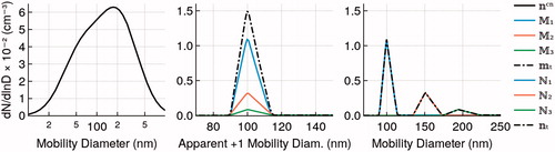
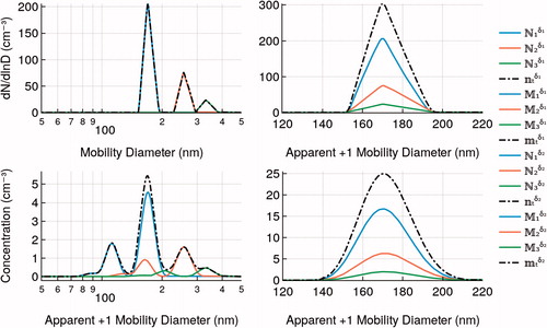
Figure 2 illustrates the distributions of a polydisperse aerosol that is transmitting through a DMA operated at a fixed voltage. The DMA selects approximately a triangular distribution around mobility centroid The distribution is symmetric when plotted against the log of mobility, but asymmetric when plotted against the log of the apparent +1 mobility diameter because the Cunningham slip flow correction factor applied in the conversion from mobility to diameter (Notebook S1) is a strong function of particle size. The majority of selected particles are singly charged, but the contribution of multiply charged particles to the total number is not negligible. The mobility distribution has contributions from particles that are at least twice the diameter of the selected centroid diameter. The relative fractions are determined by the equilibrium charge fraction and the number of particles available at each diameter.

Figure 2. Mobility classification of nominally 100 nm particles from an aerosol mobility distribution. Left panel (): assumed input bimodal lognormal size distribution. (, and ): monodisperse apparent +1 mobility size distribution. Blue, orange, and green lines represent the contribution of +1, +2, and +3 charged particles. The dashed line is the sum of the three. Right panel (, and ): same as middle panel but plotted vs. the mobility diameter. Blue, orange, and green lines represent the contribution of +1, +2, and +3 charged particles and the dashed line the sum of the three. See also Notebook S4, Figure 2 for an interactive version of this figure.

The response functions with the DMA set to voltage v corresponding to mobility z^s are computed using Equations (4)–(7). Derivations are in Notebooks S2 and S4. Transmission through the DMA is obtained from the terms of the inner sum of Equation (3)(3) (4) where is a function that evaluates to vector representing the fraction of particles carrying k charges that exit DMA as a function of diameter. The transmitted size distributions of particles carrying k charges are (5) where denotes the upstream size distribution. Particles with two or more charges have a larger mobility diameter. All multiply charged particles exit the DMA at the same mobility (or the corresponding apparent +1 mobility centroid diameter ). The multiply charged particles are shifted to the apparent +1 mobility diameter using the operator (Table 1). (6)

Equation (6)(6) evaluates to the size distribution of particles that exit the DMA at the nominal setpoint diameter. The total mobility and apparent +1 mobility distribution of all charges is obtained by summation (7)

Equations (4)–(7) are represented in JDL code as:

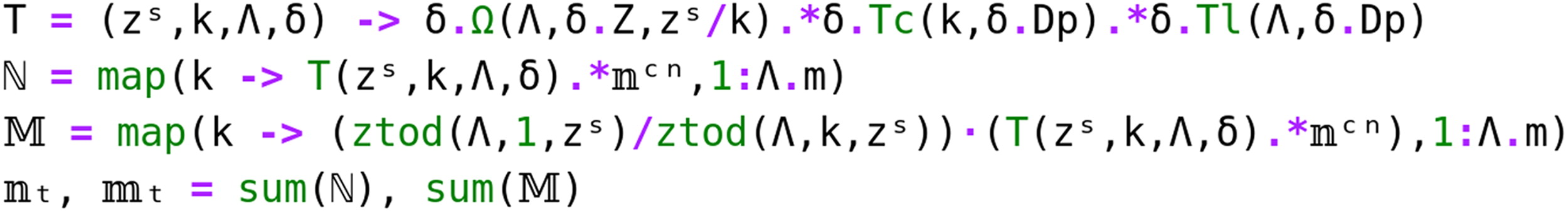where is the mapped lambda expression, converts mobility z^s to diameter assuming k charges (Notebook S1), and and evaluate to vectors of size distributions. The difference between the equations and JDL is how the DMA configuration Λ,δ is denoted. In JDL, these are explicitly passed to each function. Furthermore, JDL uses the map function to generate all and . The computational expressions are powerful because the computed vectors , and the totals and evaluate to the data type SizeDistribution. Therefore, contributions of multiply charged particles to the detector signal are assessed straightforwardly. For example, the number fraction of singly charged particles to the total can be computed as . Surface area and volume distributions or the contribution of multiply charged particles to the total volume are obtained in the usual way. Calculations for the entire size distribution are performed in Notebook S4. The selected volume concentration can be three times as large as one would calculate from a naïve estimate based on number concentration and selected diameter, e.g., , where would be the total selected number concentration as measured by a CPC downstream of the DMA.

3.2. Convolution matrix

The convolution matrix is computed via (Notebook S2) (8) where is the sum function in Table 1, m is upper number of charges to include in the inner summation of Equation (3)(3) , Z is a vector of centroid mobilities (i.e., voltages) scanned by the DMA, hcat() is a function that concatenates arrays, ^T is the matrix transpose, and … is the Julia splatting operator, which combines multiple arguments passed to the function hcat() into a single variable. The only assumption in the derivation of A is that Ω, T_c, and T_l are constant over the size bin . It may not be immediately obvious why the expression in Equation (8)(8) evaluates to the convolution matrix (or that it evaluates to a matrix at all). A step-by-step explanation is in Notebook S2. Proof of correctness of A as solution to the discretized Fredholm integral equation is deferred until later. The significance of Equation (8)(8) is that new convolution matrices can be generated by defining an appropriate , for example by adding size dependent detection efficiencies to Equation (4)(4) , or by using modified functional forms for any of its terms. For example, the convolution matrix (9) models transmission of mobility distribution through DMA 2 in tandem DMA applications where the optional charge neutralizer is not used (Figure 1). The only difference between A and O is the absence of the T_c function and that the summation is limited to one charge.

3.3. Size distribution inversion

Using A from Equation (8)(8) for inversion of size distribution data requires regularization. The regularized inverse is computed via (Hansen 2000; Twomey 1963) (10) where R is the DMA response vector to be inverted, I is the identity matrix, S is a matrix that is obtained by summing the rows of A and placing the results on the diagonal of S (Talukdar and Swihart 2003), and λ is a regularization parameter, the value of which is determined via optimization. The optimal λ is found using the L-curve method (Hansen 2000) and the iterative algorithm proposed by Talukdar and Swihart (2003). The method is implemented in JDL as the function and successfully inverts synthetic data with realistic Poisson counting error superimposed on the spectra (Notebook S5, Figure 3).

Figure 3. Right panel: reconstructed response function from 10 Hz counts. Left panel: comparison of inverted size distribution using Equation (10) and the L-curve algorithm with TSI AIM software. See Notebook S6, Figure 2 for an interactive version of this figure.

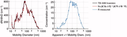
Correctness of Equations (8)(8) and (10)(10) is proved by inverting 160 ambient size distributions that were collected during one day of the SOAS campaign using the commercial TSI Inc. Model 3081 scanning mobility particle sizer (Saha et al. 2017). A response vector is constructed from the raw 10 Hz counts and inverted using Equation (10)(10) . The thus inverted data were compared to the inverted size distribution given by the manufacturer Aerosol Instrument Manager (AIM) software, assuming no diffusion correction in either method. Diffusion correction was turned off since the exact formulation of diffusion losses used in the AIM software is not available. Figure 3 demonstrates excellent correspondence between the two methods for one example spectrum. Number concentration, surface area, and volume concentration agree within for 159/160 spectra (Notebook S6, Figure 4), which is well within the spread of the inversion routine intercomparison reported by Wiedensohler et al. (2012). The L-curve algorithm failed to converge in one instance, which can be corrected by changing the initial guess of the upper and lower bounds within which λ lies. The sensitivity of the algorithm to such events depends on the structure of the L-curve, which in turn depends on the number of size bins and scan rate. Failure to converge is obvious from the noise in the proposed solution and is in principle detectable using an automated algorithm.

Figure 4. Illustration of the inversion of size and CCN distribution from a single DMA setup. Top left: simulated noisy response functions with a CPC () and a CCN () instrument as detector. Top right: inverted CN () and CCN () size distribution. Bottom left: circles are the ratio of CCN and CN response functions. The solid line corresponds to the model with parameters obtained from a least-square fit. Bottom right: circles are the ratio of CCN and CN concentration from the inverted distributions. The line corresponds the activation model using the parameters returned from a least-square fit. Note that for nm the activated fraction is set to unity and for nm is set to zero by a thresholding algorithm to eliminate noise from counting errors. See Notebook S7, Figure 3 for an interactive version of this figure.

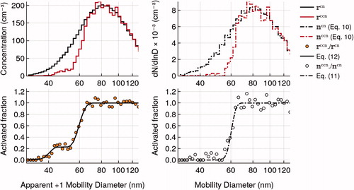
3.4. CCN response functions

A single DMA is interfaced with a CPC and a CCN instrument operated at constant water supersaturation as detectors (Cruz and Pandis 1997; Snider et al. 2006). The ratio of CCN and CN concentrations denotes the CCN response function. Petters et al. (2007) demonstrated how the CCN response function is influenced by multiply charged particles. Figure 4 illustrates the relationship between measured and inverted CCN response functions. The and are simulated data based on a 10:1 DMA sheath-to-sample flow ratio, an assumed lognormal input size distribution, a CCN activation diameter of 60 nm, Poisson counting noise that is determined by CPC and CCN sample flow rates (1 and 0.05 L min⁻¹, respectively), and bin integration time (3 s). Details are in Notebook S7. The ratio exhibits a shoulder to the left of the main activation diameter. The shoulder is caused by the activation of doubly charged particles and is present because droplet activation is proportional to particle volume. Inversion of the noisy and results in ./ with no multiply charged particle shoulder, as expected. The activation curve is generally modeled using a sigmoidal function of the authors’ choice. Petters et al. (2009) assumed a cumulative Gauss function (11)

where μ is the activation diameter, σ is the spread, is the error function, and returns a vector of activation fractions as a function of diameter. Usually, the objective is to find μ from experimental data through a minimization procedure. The fit can be obtained from either fitting (Petters et al. 2007) or ./ (Petters et al. 2009). Note that ./ is noisier than because of slight noise amplification from performing two separate inversions. It therefore is preferable to fit the model to , which heretofore required an involved fitting algorithm (Petters et al. 2007). Using JDL the model response function can be expressed as (12)

Equation (12)(12) greatly simplifies setting up the least-square minimization model to find the optimal μ and σ (Notebook S7). The black solid line in Figure 4 corresponds to Equation (12)(12) with the parameters returned from a curve fit to the synthetic data.

3.5. Hygroscopicity tandem DMA response functions

In hygroscopicity tandem DMA (Figure 1b), the first DMA is operated as a classifier with dried sample and sheath flow. The size-selected particles pass through a humdification system. Hygroscopic growth is described by the diameter growth factor , where D_dry is the selected diameter by DMA 1 and D_wet is the diameter after the humidifier. For internally mixed particles and equilibrium growth, gf is independent of D_dry, except for small differences due to a larger Kelvin effect for smaller particles. This effect is not considered here. The size and mobility distributions after the conditioner are (13) (14) (15) which is as Equations (5)–(7) but with DMA 1 selected sizes shifted by gf. The size distribution of the grown particles is measured by DMA 2 and obtained via the appropriate convolution matrix. If a charge neutralizer is placed in line (16) where are the contribution of particles carrying k charges after selection by DMA 2 to the total of the signal and is the total response function of particles exiting DMA 2. If no charge neutralizer is placed in line (17) where are the contribution of particles carrying k charges after selection by DMA 2 to the total of the signal and is the total response function of particles exiting DMA 2.

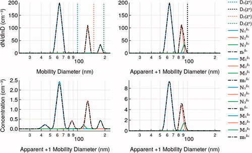
Figure 5 summarizes the distributions modeled by Equations (13)–(17). Usually no second neutralization step is performed. In a typical setup (Figure 1b), a CPC monitors concentration downstream of DMA 1. Rader and McMurry (1986) theoretically analyzed tandem DMA transfer functions. Their analysis predicts that the concentration measured by CPC 2 at the peak of the distribution is 2/3 of the concentration measured by CPC 1. The distributions from Equations (15)(15) and (17)(17) are consistent with the theoretical 2/3 ratio (Notebook S8). If the aerosol is neutralized before entering DMA 2 the response function becomes complex. The distribution in Figure 5 shows at least five discernible peaks. As shown by the partial , the second neutralization results in some peaks where only one physical size transmits through DMA 2.

Figure 5. Illustration of hygroscopicity tandem DMA response functions. Particles with nominal are selected by DMA 1. The classification step is identical to Figure 2, but with the distribution shifted by a diameter independent Blue, orange, and green solid lines denote +1, +2, and +3 charges. The dashdotted lines represent the sum of the three individual charge contributions. Top left (): mobility size distribution after transit through the humidification section. Top right (): apparent +1 mobility after transit through the humidification section. Bottom left (): response function after transit through a neutralizer and DMA 2. Bottom right (): response function after transit through DMA 2 without neutralization. See Notebook S8, Figure 3 for an interactive version of this figure.

3.6. Volatility tandem DMA response functions

Equations (13)–(17) can be applied to volatility tandem DMA with minor modifications. In volatility tandem DMA the aerosol passes through an evaporation or condensation conditioner. Here the evaporation case is discussed, but the equations below apply for either case. The evaporation rate is (18) where g subsumes terms related to molecular weight, diffusivity, vapor phase concentration, saturation vapor pressure at the particle surface, and accommodation coefficients (Bilde et al. 2003, 2015; Wright et al. 2016; Xue et al. 2005). For a fixed g, smaller particles change diameter faster than larger particles. Therefore, the evaporation factor is a vector, D_evap is the size after the conditioner and D_dry is the size after size selection by DMA 1. Transit through the volatility tandem DMA is thus modeled by replacing all terms with . Details are in Notebook S9.

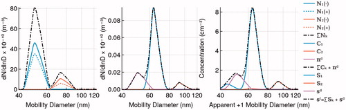
Figure 6 summarizes the volatility tandem DMA response functions. The top-left panel shows the larger shrinkage by the smaller singly charged particles relative to the larger doubly and triply charged particles. The top-right panel shows that in apparent +1 mobility space the singly charged peak has separated from the doubly and triply charged particles, thus giving the false appearance that two chemically distinct populations are present in the sample. The total response function after transit through DMA 2 without neutralization (bottom right panel) highlights that the response function is ambiguous. The +2 and +3 charged peaks do not separate. The degree of separation between the +1, +2, and +3 charged particles depends on the evaporation rate and time. With limited evaporation, the response function forms a single blurred peak, and thus derived physical properties from the response function may be in error. For this reason, Wright et al. (2016) used a second neutralizer as shown in the bottom-left panel. They identified the charge state using a CPC and aerosol electrometer as detector and tracked the shrinkage of the +2 and +1 peaks over a wide range of evaporation rates. The calculations in Figure 6 assumed a sheath-to-sample flow ratio of 10:1, which leads to excellent resolution of the different peaks. One drawback of the second neutralization step is a reduction in concentration. Decreasing the sheath-to-sample flow rate can partially offset the lower concentrations but will also degrade peak resolution. The tandem DMA model can be used as a virtual instrument to optimize the experimental configuration for resolving a particular quantity of interest. The need for such a tool for the dual tandem DMA setup discussed next was one motivation for this work.

Figure 6. Illustration of volatility tandem DMA response functions. Particles with selected by DMA 1. A constant g is used to compute the size dependent EF. The setup is identical to Figure 5, but with the distribution shifted by the vector EF. Blue, orange, and green solid lines denote +1, +2, and +3 charges. The dashdotted lines represent the sum of the three individual charge contributions. Top left (, and ): mobility size distribution after transit through the evaporation section. Top right (, and ): apparent +1 mobility distribution after transit through the evaporation section. Bottom left (): response function after transit through a neutralizer and DMA 2. Bottom right (): response function after transit through DMA 2 without neutralization. See Notebook S9, Figure 2 for an interactive version of this figure.

3.7. Dual tandem DMA response functions

Dual tandem DMA is used for the synthesis of dimers. In this system (Figure 1c, Notebook S10), the first two DMAs are operated as classifiers using power supplies of opposite polarity. The expressions (19) (20) model size selection by DMAs 1 and 2. The superscripts specify DMA number and DMA or particle polarity, i.e., denotes that DMA 1 uses a positive polarity power supply thus selecting negatively charged particles . The two aerosol flows merge into a coagulation chamber. Each population has unique and defined chemical composition, charge state (±1 or ±2) and size distribution. Chemical composition and charge state are identical for particles within any one of the distributions in Equations (19)(19) and (20)(20) . Only particles that lose their charge due to collision with ions or those that undergo coagulation with a particle carrying an equal number of opposite charges are charge neutral and transmit through the electrostatic filter. The coagulated distributions of the dimers is (Notebook S10, S11) (21) where t is time elapsed between entry and exit of the coagulation chamber, is the Brownian coagulation rate that includes correction for the attractive forces due to opposing particle charge (Zebel 1958), and accounts for the increase in sphere equivalent diameter of the formed dimers. The Brownian coagulation rate can be computed if temperature, pressure, and particle densities are known or assumed. The validity of Equation (21)(21) was tested with simulations using the particle-resolved Monte Carlo code for atmospheric aerosol simulation (PartMC, Riemer et al. 2009; Tian et al. 2017). The model is initialized with DMA-derived triangular size distributions and coagulation is simulated for 60 s. PartMC does not include the Zebel correction, and the comparison was made for uncharged dimers. The PartMC simulated dimer distribution is compared with the prediction of Equation (21)(21) . The predicted shape of the coagulated distribution is similar to the PartMC simulated distribution (Figure 4 in Notebook S11). Dimer number concentration from PartMC and Equation (21)(21) agree within a few percent for a realistic range of sheath-to-sample flow ratios, input concentrations, and selected diameters (Table 6 in Notebook S11).

Production of neutral particles due to ion collisions is assumed to follow a first order process with β^d as the decharge rate. If the collision rate is independent with size (within the bounds of the quasi-monodisperse populations), positive and negative ion concentrations are the same, the number of decharged particles remains small relative to the total population, and the decharge of multiply charged particles is negligible, then the decharge size distribution is given by (22)

The distribution is the sum of the individual coagulated distributions and the decharge distribution (). Transfer through the neutralizer and DMA 3 is obtained via the convolution matrix A (23) where is the total response function of DMA 3. Partial response functions tracking the contributions of dimers ( and the decharge particles ( are obtained analogously (Notebook S10).

Figure 7 summarizes the DMA response functions for the dual tandem DMA. The DMA flow ratios (3:1, 3:1, and 10:1 for DMAs 1, 2, and 3) and dry mobility size selection (50 nm) are based on conditions used to generate the spectrum shown in Figure 3 in Rothfuss and Petters (2016). However, neither decharge rate nor input size distribution are available from that work and these are assumed here. Calculations are limited to k = 1, 2 for clarity, because calculated +3/−3 dimer concentrations are negligible. The classifier prediction (left panel) is unremarkable other than that the negatively charged particles have higher concentration. This is due to the difference in charging probability for positively and negatively charged particles. The coagulated distributions (middle panel) are narrower than the parent size distribution due to the square dependence of the coagulation process. The distributions are also shifted by , corresponding to the sphere equivalent diameter of the dimers. The decharged particles follow the same distribution as . The overall response function after DMA 1 shows a trimodal distribution with peaks to the left and right of the +1/−1 coagulated peak. These correspond to the decharged particles and +2/−2 dimers, respectively. The response function in Figure 7 is consistent with the measured response function shown in Figure 3 in Rothfuss and Petters (2016). Since neither decharge rate nor input size distribution, nor CPC measurements downstream of DMAs 1 and 2 are available from that work, quantitative comparisons between the response model and published spectra are not possible.

Figure 7. Illustration of dual tandem DMA response functions. Left panel (): mobility distributions selected from single mobility by DMA 1 and DMA 2. Blue and orange correspond to +1, +2 charged particles. The black dashdotted line corresponds to the sum of the components. Middle panel ( and ): size distribution of particles after passage through the electrostatic filter. Blue corresponds to dimers from +1/−1 coagulation events, orange to dimers from +2/−2 coagulation events, and purple from monomer discharge. The dashdotted black line corresponds to the sum of the components. Right panel (, and ): apparent +1 mobility distribution of particles after passage through a neutralizer and DMA 3. Blue, orange, and purple correspond to size distributions of +1, +2, decharged particles in the middle panel. The black dashdotted line corresponds the sum of all components. See Figure 3 in Notebook S10 for interactive version.

Having applied the technique in published (Marsh et al. 2018; Rothfuss and Petters 2016, 2017) and not yet published studies using a range of different flow ratios, aerosol number concentrations, and upstream size distributions, we found significant variability in the observed response functions. The modeled response function from Equation (23)(23) is strongly influenced by particle number concentration, decharge rate, sheath-to-sample flow ratios in all three DMAs, and residence time in the system. All of these are to some extent controllable. However, not all are independent. For example, increasing the sheath-to-sample flow ratio increases resolution but also decreases number concentration. Increasing residence time in the coagulation chamber increases both coagulated number concentration and decharge particle concentration. Quantitative comparison of the measured response functions and the model as well as discussion on optimization of the coagulated particle signal will be the topic of a future publication. Here, Equations (19)–(23) showcase the application of JDL to a system involving 3 DMAs and a conditioner that is more complex than that of traditional tandem DMA systems. The 13 functions graphed in Figure 7 are generated with only 10 JDL expressions, excluding the setup of the DMA and upstream size distribution. This demonstrates that JDL concisely describes complex DMA configurations.

4. Discussion and conclusions

The JDL can be used to invert size distribution data, used to predict the contribution of multiply charged particles to the overall response functions, and used to model experimental setups that involve multiple DMAs. The latter is possible because no significant approximations are made to the convolution terms. In addition, the data types DMAconfig ( and DifferentialMobilityAnalyzer (δ) compartmentalize each DMA such that JDL expressions for multi-DMA setups are straightforward.

Perhaps the most powerful JDL expression is Equation (8)(8) , which represents a general computational solution of the Fredholm integral equation that requires no implementation of a numerical algorithm to solve for the matrix. Comparison with state-of-the science commercial software demonstrates that the said matrix is suitable for inverting scanning mobility particle sizer response functions using standard regularization techniques. With JDL, all terms in the convolution expression can be modified or substituted. Non-experts in computer programming can create custom-built inversions for configurations that are not supported in available software suites. For examples, using JDL matrices could be generated using the transfer function of the three monodisperse outlets DMA (Bezantakos et al. 2016) or the transfer function for DMAs that are operated with unbalanced sheath and excess flows (Stolzenburg and McMurry 2008). Transfer functions that are obtained from existing particle trajectory simulations (e.g., Collins et al. 2004; Hagwood 1999) could be invoked through a library call with very modest programming effort and no computational overhead, provided that the trajectory simulation is coded in FORTRAN or C. An example of this functionality is demonstrated in Notebook S12.

The provided size-distribution inversion algorithm is sufficiently fast (0.5–1 s execution time) such that the code could also be used for real-time data analysis in data acquisition systems. This could facilitate the construction of open-source low-cost DMA systems, e.g., by using relatively inexpensive ARM based computer architectures to interface with a data acquisition and control card and then using JDL code to process the output. All software could be without non-free licensing restrictions. However, this has not yet been attempted. A Julia interface with hardware will be needed. Two candidates to achieve such an interface would be the C-library call (Notebook S12) or the Julia-Python interface to invoke hardware-manufacturer-provided libraries. A second challenge is the robustness of the L-curve algorithm. Additional work is needed to ensure convergence in all circumstances.

The JDL source code and Jupyter notebooks are distributed as free software and these serve several purposes. Foremost, they are part of a movement toward open science. All claims and graphics made in this article are directly verifiable because they are taken from the notebooks. The worked examples can be used as a learning tool to expedite the analysis and manipulation of raw DMA data. They also serve as starting points for the development of more advanced applications. For example, Notebook S8 hints on the JDL implementation for predicting response functions for growth factor distributions, which might be further developed into a robust tandem DMA inversion. Some of the notebooks may also be used in the classroom setting to introduce students to important concepts, including size distributions, DMA theory, and regularization techniques. The public software repository is setup to encourage open community participation. Possible contributions include notebooks for classroom instruction, homework assignments using JDL, addition of DMA configurations not considered here, new inversion schemes, and improved or new functionalities of the language itself. All community contributions will retain attribution to the originating authors.

Code availability

The JDL source code, documentation, and notebooks are available as supplement or via download from https://github.com/mdpetters/DifferentialMobilityAnalyzers.jl. The GitHub repository includes installation instructions. PartMC integration requires compiled PartMC to be installed on the machine and was only tested in a Linux environment. Readers wishing to read a notebook in viewer mode are recommended to follow the web-links from the README.md file in the github repository. A virtual machine with a working copy of all software components is archived on zendo.org (doi:10.5281/zenodo.1432522). Supplementary information further describes the software architecture and includes instructions how to start the virtual machine.

Acknowledgments

The SMPS data used for validating the inversion routine were collected by Andrew Grieshop and Provat Saha during the 2013 SOAS campaign. I thank Andrew Grieshop for sharing the data file. I thank Sarah Petters, Tim Wright, and Nicholas Rothfuss for their help.

Additional information

Funding

This work was supported by the United States Department of Energy, Office of Science, Biological and Environment Research, Grant number DE-SC0018265.

References

- Alofs, D., and P. Balakumar. 1982. Inversion to obtain aerosol size distributions from measurements with a differential mobility analyzer. J. Aerosol Sci. 13(6):513–27.
- Bezanson, J., A. Edelman, S. Karpinski, and V. B. Shah. 2017. Julia: A fresh approach to numerical computing. SIAM Rev. 59(1):65–98.
- Bezantakos, S., M. Giamarelou, L. Huang, J. Olfert, and G. Biskos. 2016. Modification of the TSI 3081 differential mobility analyzer to include three monodisperse outlets: Comparison between experimental and theoretical performance. Aerosol Sci. Technol. 50(12):1342–51.
- Bilde, M., K. Barsanti, M. Booth, C. D. Cappa, N. M. Donahue, E. U. Emanuelsson, G. McFiggans, U. K. Krieger, C. Marcolli, D. Topping, et al. 2015. Saturation vapor pressures and transition enthalpies of low-volatility organic molecules of atmospheric relevance: From dicarboxylic acids to complex mixtures. Chem. Rev. 115(10):4115–56. PMID: 25929792.
- Bilde, M., B. Svenningsson, J. Mønster, and T. Rosenørn. 2003. Even-odd alternation of evaporation rates and vapor pressures of C3–C9 dicarboxylic acid aerosols. Environ. Sci. Technol. 37(7):1371–8.
- Collins, D. R., D. R. Cocker, R. C. Flagan, and J. H. Seinfeld. 2004. The scanning DMA transfer function. Aerosol Sci. Technol. 38(8):833–50.
- Cruz, C. N., and S. N. Pandis. 1997. A study of the ability of pure secondary organic aerosol to act as cloud condensation nuclei. Atmos. Environ. 31(15):2205–14.
- DeMott, P. J., M. D. Petters, A. J. Prenni, C. M. Carrico, S. M. Kreidenweis, J. L. Collett, and H. Moosmüller. 2009. Ice nucleation behavior of biomass combustion particles at cirrus temperatures. J. Geophys. Res.: Atmos. 114:D16205.
- Flagan, R. C. 1998. History of electrical aerosol measurements. Aerosol Sci. Technol. 28(4):301–80.
- Gysel, M., G. McFiggans, and H. Coe. 2009. Inversion of tandem differential mobility analyser (TDMA) measurements. J. Aerosol Sci. 40(2):134–51.
- Hagwood, C. 1999. The DMA transfer function with Brownian motion a trajectory/Monte-Carlo approach. Aerosol Sci. Technol. 30(1):40–61.
- Hansen, P. C. 2000. The L-curve and its use in the numerical treatment of inverse problems. In Computational inverse problems in electrocardiology, ed. P. Johnston, Advances in computational bioengineering, 119–42. Southampton: WIT Press.
- Hewitt, G. W. 1957. The charging of small particles for electrostatic precipitation. Trans. Am. Inst. Electr. Eng Part I: Commun. Electron. 76(3):300–6.
- Kandlikar, M., and G. Ramachandran. 1999. Inverse methods for analysing aerosol spectrometer measurements: A critical review. J. Aerosol Sci. 30(4):413–37.
- Knutson, E., and K. Whitby. 1975. Aerosol classification by electric mobility: Apparatus, theory, and applications. J. Aerosol Sci. 6(6):443–51.
- Langer, G., J. Pierrard, and G. Yamate. 1964. Further development of an electrostatic classifier for submicron airborne particles. Air Water Pollut. 8:167–76.
- Larriba, C., C. J. Hogan, M. Attoui, R. Borrajo, J. F. Garcia, and J. F. de la Mora. 2011. The mobility-volume relationship below 3.0 nm examined by tandem mobility-mass measurement. Aerosol Sci. Technol. 45(4):453–67.
- Liu, B. Y., and D. Y. Pui. 1974. A submicron aerosol standard and the primary absolute calibration of the condensation nuclei counter. J. Colloid Interface Sci. 47(1):155–71.
- Maisels, A., F. E. Kruis, H. Fissan, B. Rellinghaus, and H. Zähres. 2000. Synthesis of tailored composite nanoparticles in the gas phase. Appl. Phys. Lett. 77(26):4431–3.
- Marsh, A., S. S. Petters, N. E. Rothfuss, G. Rovelli, Y. C. Song, J. P. Reid, and M. D. Petters. 2018. Amorphous phase state diagrams and viscosity of ternary aqueous organic/organic and inorganic/organic mixtures, Phys. Chem. Chem. Phys. 20:15086–15097. doi:10.1039/C8CP00760H.
- Park, K., D. Dutcher, M. Emery, J. Pagels, H. Sakurai, J. Scheckman, S. Qian, M. R. Stolzenburg, X. Wang, J. Yang, and P. H. McMurry. 2008. Tandem measurements of aerosol properties—A review of mobility techniques with extensions. Aerosol Sci. Technol. 42(10):801–16.
- Petters, M. D., C. M. Carrico, S. M. Kreidenweis, A. J. Prenni, P. J. DeMott, J. L. Collett, and H. Moosmüller. 2009. Cloud condensation nucleation activity of biomass burning aerosol. J. Geophys. Res.: Atmos. 114:D22205.
- Petters, M. D., A. J. Prenni, S. M.Kreidenweis, and P. J.DeMott. 2007. On measuring the critical diameter of cloud condensation nuclei using mobility selected aerosol. Aerosol Sci. Technol. 41(10):907–13.
- Pfeifer, S., W. Birmili, A. Schladitz, T. Müller, A. Nowak, and A. Wiedensohler. 2014. A fast and easy-to-implement inversion algorithm for mobility particle size spectrometers considering particle number size distribution information outside of the detection range. Atmos. Meas. Tech. 7(1):95–105.
- Rader, D., and P. McMurry. 1986. Application of the tandem differential mobility analyzer to studies of droplet growth or evaporation. J. Aerosol Sci. 17(5):771–87.
- Reineking, A., and J. Porstendörfer. 1986. Measurements of particle loss functions in a differential mobility analyzer (TSI, model 3071) for different flow rates. Aerosol Sci. Technol. 5(4):483–6.
- Riemer, N., M. West, R. A. Zaveri, and R. C. Easter. 2009. Simulating the evolution of soot mixing state with a particle resolved aerosol model. J. Geophys. Res.: Atmos. 114:D09202.
- Rothfuss, N. E., and M. D. Petters. 2016. Coalescence-based assessment of aerosol phase state using dimers prepared through a dual-differential mobility analyzer technique. Aerosol Sci. Technol. 50(12):1294–305.
- Rothfuss, N. E., and M. D. Petters. 2017. Characterization of the temperature and humidity-dependent phase diagram of amorphous nanoscale organic aerosols. Phys. Chem. Chem. Phys. 19(9):6532–45.
- Saha, P. K., A. Khlystov, K. Yahya, Y. Zhang, L. Xu, N. L. Ng, and A. P. Grieshop. 2017. Quantifying the volatility of organic aerosol in the southeastern US. Atmos. Chem. Phys. 17(1):501–20.
- Snider, J. R., M. D. Petters, P. Wechsler, and P. S. K. Liu. 2006. Supersaturation in the Wyoming CCN instrument. J. Atmos. Ocean. Technol. 23(10):1323–39.
- Stolzenburg, M., and P. McMurry. 1988. TDMAfit user’s manual. Technical Report (PTL Publication No. 653).
- Stolzenburg, M. R., and P. H. McMurry. 2008. Equations governing single and tandem DMA configurations and a new lognormal approximation to the transfer function. Aerosol Sci. Technol. 42(6):421–32.
- Stolzenburg, M. R., and P. H. McMurry. 2018. Accuracy of recovered moments for narrow mobility distributions obtained with commonly used inversion algorithms for mobility size spectrometers. Aerosol Sci. Technol. 52(6):614–25.
- Stratmann, F., T. Kauffeldt, D. Hummes, and H. Fissan. 1997. Differential electrical mobility analysis: a theoretical study. Aerosol Sci. Technol. 26(4):368–83.
- Talukdar, S. S., and M. T. Swihart. 2003. An improved data inversion program for obtaining aerosol size distributions from scanning differential mobility analyzer data. Aerosol Sci. Technol. 37(2):145–61.
- Tian, J., B. T. Brem, M. West, T. C. Bond, M. J. Rood, and N. Riemer. 2017. Simulating aerosol chamber experiments with the particle resolved aerosol model PartMC. Aerosol Sci. Technol. 51(7):856–67.
- TSI. 2009. Series 3080 electrostatic classifiers operation and service manual. Revision j ed. Shoreview, MN: TSI Incorporated.
- Twomey, S. 1963. On the numerical solution of fredholm integral equations of the first kind by the inversion of the linear system produced by quadrature. J. ACM 10(1):97–101.
- Wang, S. C., and R. C. Flagan. 1990. Scanning electrical mobility spectrometer. Aerosol Sci. Technol. 13(2):230–40.
- Wiedensohler, A. 1988. An approximation of the bipolar charge distribution for particles in the submicron size range. J. Aerosol Sci. 19(3):387–9.
- Wiedensohler, A., W. Birmili, A. Nowak, A. Sonntag, K. Weinhold, M. Merkel, B. Wehner, T. Tuch, S. Pfeifer, M. Fiebig, et al. 2012. Mobility particle size spectrometers: Harmonization of technical standards and data structure to facilitate high quality long-term observations of atmospheric particle number size distributions. Atmos. Meas. Tech. 5(3):657–85.
- Wiedensohler, A., and H. Fissan. 1988. Aerosol charging in high purity gases. Sixteenth Annual Conference of the Gesellschaft fur Aerosolforschung. J. Aerosol Sci. 19(7):867–70.
- Wiedensohler, A., E. Lütkemeier, M. Feldpausch, and C. Helsper. 1986. Investigation of the bipolar charge distribution at various gas conditions. J. Aerosol Sci. 17(3):413–6.
- Wright, T. P., C. Song, S. Sears, and M. D. Petters. 2016. Thermodynamic and kinetic behavior of glycerol aerosol. Aerosol Sci. Technol. 50(12):1385–96.
- Xue, H., A. M. Moyle, N. Magee, J. Y. Harrington, and D. Lamb. 2005. Experimental studies of droplet evaporation kinetics: Validation of models for binary and ternary aqueous solutions. J. Atmos. Sci. 62(12):4310–26.
- Zebel, G. 1958. Zur theorie des verhaltens elektrisch geladener aerosole. Kolloid-Zeitschrift 157(1):37–50.
- Zhang, S.-H., Y. Akutsu, L. M. Russell, R. C. Flagan, and J. H. Seinfeld. 1995. Radial differential mobility analyzer. Aerosol Sci. Technol. 23(3):357–72.