Extended log-normal method of moments for solving the population balance equation for Brownian coagulation

Abstract

An extended log-normal method of moments (ELNMOM) is presented in this study for solving the population balance equation (PBE) for Brownian coagulation. The method is an extension of the log-normal method of moments (LNMOM) proposed by Lee in 1983. The ELNMOM uses the superposition of log-normal subdistributions to represent the size distribution. Unlike previous modal studies, the subdistributions are not independent modes but flexible components in this study and the closure of this method is achieved by introducing additional higher-order moment equations. Based on some simplifying assumptions, the ELNMOM is implemented with only four adjustable parameters for a preliminary exploration. The method is then validated by comparing the size distribution parameters predicted by this method with those predicted by the LNMOM and other numerical methods for Brownian coagulation in the continuum regime and the free-molecular regime. The results show that the ELNMOM more accurately predicts the total particle number concentration, the geometric standard deviation and the geometric mean particle volume than the LNMOM while not taking much more computation time.

Copyright © 2019 American Association for Aerosol Research

1. Introduction

Population balance modeling has become an increasingly important research topic due to its many applications in environmental and engineering particulate systems (Mann et al. 2010; Palaniswaamy and Loyalka 2008; Ramkrishna and Singh 2014; Shekar et al. 2012). Particle coagulation plays an important role in determining the particle size distributions for these particulate systems. The time evolution of the size distribution due to coagulation is described by the population balance equation (PBE). The integral-differential PBE was first proposed by Müller (1928) based on the fundamental work of Smoluchowski (1918). Due to the highly non-linear nature of the PBE, there are only a limited number of analytical solutions in the literature (Wang, Peng, and Yu 2019; Xie and He 2013). Thus, various numerical methods have been proposed for solving the PBE, which can be categorized as the sectional method (SM) (Gelbard, Tambour, and Seinfeld 1980; Kumar et al. 2006; Landgrebe and Pratsinis 1990), the method of moments (MOM) (Frenklach and Harris 1987; Marchisio and Fox 2005; McGraw 1997; Yu, Lin, and Chan 2008), and the Monte Carlo method (Kruis, Maisels, and Fissan 2000; Zhao and Zheng 2013). These numerical methods are still being developed and expanded to improve their accuracy and efficiency.

The MOM has been extensively used due to its simple implementation and high efficiency. In the MOM framework, the PBE is converted into an infinite set of moment equations. However, only a finite number of moment equations can be numerically solved. Thus, a closure problem results from representing the other moments in terms of the finite set of moments to be solved. The MOM can be divided into several methods based on the closure techniques, such as the log-normal MOM (LNMOM) (Lee 1983), the pth-order polynomial MOM (Barrett and Jheeta 1996), the quadrature-based MOM (Marchisio and Fox 2005; McGraw 1997), the MOM with interpolative closure (Frenklach 2002), and the Taylor series expansion MOM (TEMOM) (Yu, Lin, and Chan 2008). The LNMOM assumes a time-dependent log-normal size distribution with three adjustable parameters. This method is very efficient and easy to implement due to the simple closure, which makes it widely used in aerosol dynamics modeling (Kajino 2011; Park and Lee 2002; Pratsinis 1988). However, the accuracy and application of the LNMOM are limited by the assumed form of the distribution. Previous studies have shown that the method tends to underestimate the geometric standard deviation of the size distribution for Brownian coagulation (Park and Lee 2002; Park, Xiang, and Lee 2000). In addition, the LNMOM fails to give reasonable predictions for simultaneous particle nucleation and coagulation because a bimodal distribution develops (Megaridis and Dobbins 1990). As a comparison, the other MOMs do not make prior assumptions on the size distribution form. These methods can accurately and efficiently track the time evolution of the moments and have been extensively used to solve various particle processes. However, the distribution reconstruction from the moments is still unsolved because the finite set of moments does not result in a unique distribution (Diemer and Olson 2002; John et al. 2007). Since the size distribution characteristics are of great interest in many fields, we focus on the MOMs with a prior size distribution.

The accuracy of the LNMOM cannot be improved if the log-normal form of the size distribution is not changed. A number of studies have focused on modifying the distribution form for various purposes, which can be divided into two types. One is to change the single log-normal distribution function (Seo and Brock 1990; Yamamoto 2004) while the other is to use the superposition of two or more distinct log-normal subdistributions. The latter approach is more general than the former one and has been widely used to simulate modal aerosol dynamics (MAD) (Megaridis and Dobbins 1990; Whitby and McMurry 1997; Yu and Chan 2015). However, the solution method for the MAD model requires an assigning scheme for inter-modal and intra-modal coagulation to separate different modes, which may be problematic in some cases (Jeong and Choi 2004). In addition, the superposition approach should not only limit to multimodal distributions. For example, a unimodal distribution can also be represented by the superposition of two or more log-normal subdistributions. Thus, we consider the superposition approach in a different way from previous modal studies.

This study presents an extended log-normal method of moments (ELNMOM) as an extension to the LNMOM. The ELNMOM uses the superposition of log-normal subdistributions to represent the size distribution. Unlike the MAD model (Whitby and McMurry 1997), the subdistributions are not regarded as independent modes in this study and the moment closure is achieved by introducing additional higher-order moments rather than using the assigning scheme. We implement the simplest version of the ELNMOM with four adjustable parameters. The conversion between moments and the four parameters is strictly derived. Then the ELNMOM is validated by comparing the predicted size distribution parameters with those of the LNMOM, the TEMOM and the SM for Brownian coagulation in the continuum regime and the free-molecular regime. The computation time of these methods is also compared to illustrate the calculation efficiency of the ELNMOM.

2. Theory

The continuous integral-differential PBE that governs the time evolution of particle size distributions due to coagulation is expressed as (Müller 1928) (1) $$\frac{\partial n(v,t)}{\partial t}=\frac{1}{2}{\int }_0^v\beta (v-\overline{v},\overline{v})n(v-\overline{v},t)n(\overline{v},t)d\overline{v}-n(v,t){\int }_0^{\infty }\beta (v,\overline{v})n(\overline{v},t)d\overline{v},$$(1) where, $n(v,t)dv$ is the particle number concentration with particle volumes between $v$ and $v+dv$ at time $t$ and $\beta (v,\overline{v})$ is the collision kernel for two particles with volumes $v$ and $\overline{v}$.

The $k$th moment of the particle size distribution in the volume space is defined as (2) $$M_k={\int }_0^{\infty }{v}^{k}n(v,t)dv,$$(2) where, $k$ is an arbitrary real number. The moment equation can be obtained by multiplying Equation (1)(1) $$\frac{\partial n(v,t)}{\partial t}=\frac{1}{2}{\int }_0^v\beta (v-\overline{v},\overline{v})n(v-\overline{v},t)n(\overline{v},t)d\overline{v}-n(v,t){\int }_0^{\infty }\beta (v,\overline{v})n(\overline{v},t)d\overline{v},$$(1) with $v^k$ and then integrating from 0 to ∞: (3) $$\frac{d{M}_k}{dt}=\frac{1}{2}{\int }_0^{\infty }{\int }_0^{\infty }({(v+\overline{v})}^k-v^k-{\overline{v}}^k)\beta (v,\overline{v}\left)n\right(v,t\left)n\right(\overline{v},t)dvd\overline{v}.$$(3)

The right side of Equation (3)(3) $$\frac{d{M}_k}{dt}=\frac{1}{2}{\int }_0^{\infty }{\int }_0^{\infty }({(v+\overline{v})}^k-v^k-{\overline{v}}^k)\beta (v,\overline{v}\left)n\right(v,t\left)n\right(\overline{v},t)dvd\overline{v}.$$(3) can be expanded into moments of different orders for a given collision kernel. Thus, the PBE is converted into a system of ordinary differential equation (ODEs) for the moments. A closure model is needed for these moments since only a limited set of moments is directly solved.

2.1. Brief review of the LNMOM

The LNMOM assumes a time-dependent log-normal function for the size distribution during coagulation (Lee 1983): (4) $$n(v,t)=\frac{N\left(t\right)}{3\sqrt{2\pi }v\hspace{0.17em}\text{ln}\hspace{0.17em}\sigma \left(t\right)}\text{exp}[-\frac{{\hspace{0.17em}\text{ln}\hspace{0.17em}}^2(v/v_g(t\left)\right)}{18{\hspace{0.17em}\text{ln}\hspace{0.17em}}^2\sigma \left(t\right)}],$$(4) where, $N(t)$ is the total particle number concentration, $\sigma (t)$ is the geometric standard deviation based on the particle diameter, and $v_g(t)$ is the geometric number mean particle volume. According to the properties of a log-normal function, all the moments can be expressed in terms of $N$, $\sigma$ and $v_g$ as (5) $$M_k=N{v}_g^k\hspace{0.17em}\text{exp}\hspace{0.17em}(\frac{9}{2}{k}^2{\hspace{0.17em}\text{ln}\hspace{0.17em}}^2\sigma ).$$(5)

Moreover, $N$, $\sigma$ and $v_g$ can be expressed in terms of the first three moments, $M_0$, $M_1$ and $M_2$, as (6) $$N=M_0,$$(6)

(7) $$\sigma =\hspace{0.17em}\text{exp}[\sqrt{\hspace{0.17em}\text{ln}\hspace{0.17em}(M_0{M}_2/M_1^2)}/3],$$(7) (8) $$v_g=M_1^2/\left(M_0^{3/2}{M}_2^{1/2}\right).$$(8)

Thus, all the moments are functions of $M_0$, $M_1$ and $M_2$. The closure of the LNMOM is achieved by solving the first three moment equations ($k$=0, 1 and 2) with the moment conversion shown in Equations (5)–(8).

2.2. Extended log-normal method of moments (ELNMOM)

The ELNMOM assumes that an actual size distribution can be regarded as a superposition of log-normal subdistributions. Unlike the MAD model (Whitby and McMurry 1997), the subdistributions are not distinguished as independent modes here. In contrast, they represent flexible components that can form either a unimodal distribution or a multimodal distribution based on the relative positions. Each subdistribution is described by three size distribution parameters, as shown in Equation (4)(4) $$n(v,t)=\frac{N\left(t\right)}{3\sqrt{2\pi }v\hspace{0.17em}\text{ln}\hspace{0.17em}\sigma \left(t\right)}\text{exp}[-\frac{{\hspace{0.17em}\text{ln}\hspace{0.17em}}^2(v/v_g(t\left)\right)}{18{\hspace{0.17em}\text{ln}\hspace{0.17em}}^2\sigma \left(t\right)}],$$(4) . If there are $m$ ($m\ge 2$) subdistributions, the generalized size distribution function is expressed as (9) $$n(v,t)=\sum _{i=1}^m{n}_i(v,t)=\sum _{i=1}^m\frac{N_i\left(t\right)}{3\sqrt{2\pi }v\hspace{0.17em}\text{ln}\hspace{0.17em}{\sigma }_i\left(t\right)}\text{exp}[-\frac{{\hspace{0.17em}\text{ln}\hspace{0.17em}}^2(v/v_{gi}(t\left)\right)}{18{\hspace{0.17em}\text{ln}\hspace{0.17em}}^2{\sigma }_i\left(t\right)}],$$(9) where $N_i$, ${\sigma }_i$ and $v_{gi}$ are the size distribution parameters of the $i$th subdistribution. Based on Equations (5)(5) $$M_k=N{v}_g^k\hspace{0.17em}\text{exp}\hspace{0.17em}(\frac{9}{2}{k}^2{\hspace{0.17em}\text{ln}\hspace{0.17em}}^2\sigma ).$$(5) and (9)(9) $$n(v,t)=\sum _{i=1}^m{n}_i(v,t)=\sum _{i=1}^m\frac{N_i\left(t\right)}{3\sqrt{2\pi }v\hspace{0.17em}\text{ln}\hspace{0.17em}{\sigma }_i\left(t\right)}\text{exp}[-\frac{{\hspace{0.17em}\text{ln}\hspace{0.17em}}^2(v/v_{gi}(t\left)\right)}{18{\hspace{0.17em}\text{ln}\hspace{0.17em}}^2{\sigma }_i\left(t\right)}],$$(9) , the moments of the generalized size distribution are expressed as (10) $$M_k=\sum _{i=1}^m{N}_i{v}_{gi}^k\hspace{0.17em}\text{exp}\hspace{0.17em}\left(\frac{9}{2}{k}^2{\hspace{0.17em}\text{ln}\hspace{0.17em}}^2{\sigma }_i\right).$$(10)

Since there are $3m$ size distribution parameters, $3m$ moment equations are needed for the closure. The difficulty is that the conversion between moments and the size distribution parameters is very complex. Thus, we first focus on $m=2$ for a preliminary exploration.

For $m=2$, there are six parameters, $N_1$, ${\sigma }_1$, $v_{g1}$, $N_2$, ${\sigma }_2$ and $v_{g2}$, for the two subdistributions. However, the analytical manipulation to represent these parameters in terms of moments is still difficult. From the view of superposition, $v_g$ has the biggest influence because it represents the position of the distribution on the $v$ axis. Thus, the simplest version of the ELNMOM is that the two subdistributions have the same $N$ and $\sigma$ but different $v_g$. In this case, the extended size distribution has four adjustable parameters and can be expressed as (11) $$n(v,t)=\frac{N\left(t\right)}{6\sqrt{2\pi }v\hspace{0.17em}\text{ln}\hspace{0.17em}{\sigma }^{\prime }\left(t\right)}[\text{exp}\hspace{0.17em}(-\frac{{\hspace{0.17em}\text{ln}\hspace{0.17em}}^2(v/v_{g1}(t\left)\right)}{18{\hspace{0.17em}\text{ln}\hspace{0.17em}}^2{\sigma }^{\prime }\left(t\right)})+\hspace{0.17em}\text{exp}\hspace{0.17em}(-\frac{{\hspace{0.17em}\text{ln}\hspace{0.17em}}^2(v/v_{g2}(t\left)\right)}{18{\hspace{0.17em}\text{ln}\hspace{0.17em}}^2{\sigma }^{\prime }\left(t\right)}\left)\right],$$(11) where, ${\sigma }^{\prime }(t)$ is the geometric standard deviation of the subdistribution and $v_{g1}(t)$ and $v_{g2}(t)$ are the geometric number mean particle volumes of the first and second subdistributions.

Although $N$ still represents the total particle number concentration, ${\sigma }^{\prime }$, $v_{g1}$ and $v_{g2}$ are the parameters of the two subdistributions. The equivalent $\sigma$ and $v_g$ of the extended size distribution can be calculated from Equation (11)(11) $$n(v,t)=\frac{N\left(t\right)}{6\sqrt{2\pi }v\hspace{0.17em}\text{ln}\hspace{0.17em}{\sigma }^{\prime }\left(t\right)}[\text{exp}\hspace{0.17em}(-\frac{{\hspace{0.17em}\text{ln}\hspace{0.17em}}^2(v/v_{g1}(t\left)\right)}{18{\hspace{0.17em}\text{ln}\hspace{0.17em}}^2{\sigma }^{\prime }\left(t\right)})+\hspace{0.17em}\text{exp}\hspace{0.17em}(-\frac{{\hspace{0.17em}\text{ln}\hspace{0.17em}}^2(v/v_{g2}(t\left)\right)}{18{\hspace{0.17em}\text{ln}\hspace{0.17em}}^2{\sigma }^{\prime }\left(t\right)}\left)\right],$$(11) as (12) $$\sigma =\hspace{0.17em}\text{exp}\hspace{0.17em}(\sqrt{{\hspace{0.17em}\text{ln}\hspace{0.17em}}^2(v_{g1}/v_{g2})/4+9{\hspace{0.17em}\text{ln}\hspace{0.17em}}^2{\sigma }^{\prime }}/3),$$(12)

(13) $$v_g=\sqrt{v_{g1}{v}_{g2}}.$$(13)

If $v_{g1}=v_{g2}$, then $\sigma ={\sigma }^{\prime }$ from Equation (12)(12) $$\sigma =\hspace{0.17em}\text{exp}\hspace{0.17em}(\sqrt{{\hspace{0.17em}\text{ln}\hspace{0.17em}}^2(v_{g1}/v_{g2})/4+9{\hspace{0.17em}\text{ln}\hspace{0.17em}}^2{\sigma }^{\prime }}/3),$$(12) . In this case, Equation (11)(11) $$n(v,t)=\frac{N\left(t\right)}{6\sqrt{2\pi }v\hspace{0.17em}\text{ln}\hspace{0.17em}{\sigma }^{\prime }\left(t\right)}[\text{exp}\hspace{0.17em}(-\frac{{\hspace{0.17em}\text{ln}\hspace{0.17em}}^2(v/v_{g1}(t\left)\right)}{18{\hspace{0.17em}\text{ln}\hspace{0.17em}}^2{\sigma }^{\prime }\left(t\right)})+\hspace{0.17em}\text{exp}\hspace{0.17em}(-\frac{{\hspace{0.17em}\text{ln}\hspace{0.17em}}^2(v/v_{g2}(t\left)\right)}{18{\hspace{0.17em}\text{ln}\hspace{0.17em}}^2{\sigma }^{\prime }\left(t\right)}\left)\right],$$(11) reduces to Equation (4)(4) $$n(v,t)=\frac{N\left(t\right)}{3\sqrt{2\pi }v\hspace{0.17em}\text{ln}\hspace{0.17em}\sigma \left(t\right)}\text{exp}[-\frac{{\hspace{0.17em}\text{ln}\hspace{0.17em}}^2(v/v_g(t\left)\right)}{18{\hspace{0.17em}\text{ln}\hspace{0.17em}}^2\sigma \left(t\right)}],$$(4) , which indicates that the log-normal size distribution is a special case of the extended size distribution. Figure 1 schematically shows the various types of size distributions generated from Equation (11)(11) $$n(v,t)=\frac{N\left(t\right)}{6\sqrt{2\pi }v\hspace{0.17em}\text{ln}\hspace{0.17em}{\sigma }^{\prime }\left(t\right)}[\text{exp}\hspace{0.17em}(-\frac{{\hspace{0.17em}\text{ln}\hspace{0.17em}}^2(v/v_{g1}(t\left)\right)}{18{\hspace{0.17em}\text{ln}\hspace{0.17em}}^2{\sigma }^{\prime }\left(t\right)})+\hspace{0.17em}\text{exp}\hspace{0.17em}(-\frac{{\hspace{0.17em}\text{ln}\hspace{0.17em}}^2(v/v_{g2}(t\left)\right)}{18{\hspace{0.17em}\text{ln}\hspace{0.17em}}^2{\sigma }^{\prime }\left(t\right)}\left)\right],$$(11) . The extended size distribution can be a log-normal distribution, a broad unimodal distribution or a bimodal distribution based on the relative positions. Thus, the extended size distribution function can represent a wider set of size distributions than the log-normal distribution function.

Figure 1. Various types of size distributions generated from Equation (11)(11) $$n(v,t)=\frac{N\left(t\right)}{6\sqrt{2\pi }v\hspace{0.17em}\text{ln}\hspace{0.17em}{\sigma }^{\prime }\left(t\right)}[\text{exp}\hspace{0.17em}(-\frac{{\hspace{0.17em}\text{ln}\hspace{0.17em}}^2(v/v_{g1}(t\left)\right)}{18{\hspace{0.17em}\text{ln}\hspace{0.17em}}^2{\sigma }^{\prime }\left(t\right)})+\hspace{0.17em}\text{exp}\hspace{0.17em}(-\frac{{\hspace{0.17em}\text{ln}\hspace{0.17em}}^2(v/v_{g2}(t\left)\right)}{18{\hspace{0.17em}\text{ln}\hspace{0.17em}}^2{\sigma }^{\prime }\left(t\right)}\left)\right],$$(11) .

Since the extended size distribution has four parameters, the third moment, $M_3$, is introduced in addition to the first three moments, $M_0$, $M_1$ and $M_2$. According to Equations (10)(10) $$M_k=\sum _{i=1}^m{N}_i{v}_{gi}^k\hspace{0.17em}\text{exp}\hspace{0.17em}\left(\frac{9}{2}{k}^2{\hspace{0.17em}\text{ln}\hspace{0.17em}}^2{\sigma }_i\right).$$(10) and (11)(11) $$n(v,t)=\frac{N\left(t\right)}{6\sqrt{2\pi }v\hspace{0.17em}\text{ln}\hspace{0.17em}{\sigma }^{\prime }\left(t\right)}[\text{exp}\hspace{0.17em}(-\frac{{\hspace{0.17em}\text{ln}\hspace{0.17em}}^2(v/v_{g1}(t\left)\right)}{18{\hspace{0.17em}\text{ln}\hspace{0.17em}}^2{\sigma }^{\prime }\left(t\right)})+\hspace{0.17em}\text{exp}\hspace{0.17em}(-\frac{{\hspace{0.17em}\text{ln}\hspace{0.17em}}^2(v/v_{g2}(t\left)\right)}{18{\hspace{0.17em}\text{ln}\hspace{0.17em}}^2{\sigma }^{\prime }\left(t\right)}\left)\right],$$(11) , all the moments can be expressed in terms of $N$, ${\sigma }^{\prime }$, $v_{g1}$ and $v_{g2}$ as (14) $$M_k=\frac{1}{2}N(v_{g1}^k+v_{g2}^k)\hspace{0.17em}\text{exp}\hspace{0.17em}\left(\frac{9}{2}{k}^2{\hspace{0.17em}\text{ln}\hspace{0.17em}}^2{\sigma }^{\prime }\right).$$(14)

Moreover, $N$, ${\sigma }^{\prime }$, $v_{g1}$ and $v_{g2}$ can be obtained from the first four moments, $M_0$, $M_1$, $M_2$ and $M_3$, as (15) $$N=M_0,$$(15)

(16) $${\sigma }^{\prime }=\hspace{0.17em}\text{exp}\hspace{0.17em}(\sqrt{\hspace{0.17em}\text{ln}\hspace{0.17em}{x}_0}/3),$$(16) (17) $$v_{g1}=\frac{M_1}{M_0\sqrt{x_0}}(1-\sqrt{\frac{M_0{M}_2}{M_1^2{x}_0}-1}),$$(17) (18) $$v_{g2}=\frac{M_1}{M_0\sqrt{x_0}}(1+\sqrt{\frac{M_0{M}_2}{M_1^2{x}_0}-1}).$$(18)

where $x_0$ is the second real root (sorted in descending order) of the cubic equation, $f(x)=2M_1^3{x}^3-3M_0{M}_1{M}_2{x}^2+M_0^2{M}_3=0$. Detailed derivations of Equations (15)–(18) are given in online supplemental information (SI). Thus, all the moments are functions of $M_0$, $M_1$, $M_2$ and $M_3$. The closure of the ELNMOM is achieved by solving the first four moment equations ($k$=0, 1, 2 and 3) with the moment conversion shown in Equations (14)–(18).

2.3. Moment equations for Brownian coagulation

The first four moment equations for Brownian coagulation in the continuum regime and the free-molecular regime are derived here. The collision kernel for Brownian coagulation in the continuum regime is expressed as (Lee 1983) (19) $$\beta (v,\overline{v})=K_{co}(v^{1/3}+{\overline{v}}^{1/3})(1/v^{1/3}+1/{\overline{v}}^{1/3}),$$(19) where $K_{co}$ is the collision coefficient ($K_{co}=2k_{B}T/3\mu$), $k_B$ is the Boltzmann constant, $T$ is the gas temperature and $\mu$ is the gas viscosity.

Substituting Equation (19)(19) $$\beta (v,\overline{v})=K_{co}(v^{1/3}+{\overline{v}}^{1/3})(1/v^{1/3}+1/{\overline{v}}^{1/3}),$$(19) into Equation (3)(3) $$\frac{d{M}_k}{dt}=\frac{1}{2}{\int }_0^{\infty }{\int }_0^{\infty }({(v+\overline{v})}^k-v^k-{\overline{v}}^k)\beta (v,\overline{v}\left)n\right(v,t\left)n\right(\overline{v},t)dvd\overline{v}.$$(3) for $k$=0, 1, 2 and 3 gives (20) $$\frac{d{M}_0}{dt}=-K_{co}(M_0^2+M_{1/3}{M}_{-1/3}),$$(20)

(21) $$\frac{d{M}_1}{dt}=0,$$(21) (22) $$\frac{d{M}_2}{dt}=2K_{co}(M_1^2+M_{4/3}{M}_{2/3}),$$(22) (23) $$\frac{d{M}_3}{dt}=3K_{co}(2M_2{M}_1+M_{7/3}{M}_{2/3}+M_{5/3}{M}_{4/3}).$$(23)

With Equations (14)–(18) and Equations (20)–(23), the time evolution of the size distribution due to Brownian coagulation in the continuum regime can be numerically solved using an ODE solver.

The collision kernel for Brownian coagulation in the free-molecular regime is expressed as (Lee, Chen, and Gieseke 1984) (24) $$\beta (v,\overline{v})=K_{fm}{(v^{1/3}+{\overline{v}}^{1/3})}^2{(1/v+1/\overline{v})}^{1/2},$$(24) where $K_{fm}$ is the collision coefficient ($K_{fm}=(3/4\pi {)}^{1/6}{(6k_{B}T/{\rho }_p)}^{1/2}$) and ${\rho }_p$ is the particle density. The right side of Equation (24)(24) $$\beta (v,\overline{v})=K_{fm}{(v^{1/3}+{\overline{v}}^{1/3})}^2{(1/v+1/\overline{v})}^{1/2},$$(24) cannot be directly expanded into terms of the form $v^i{\overline{v}}^j$ ($i$ and $j$ are arbitrary real numbers) because of the square root. Lee, Chen, and Gieseke (1984) introduced the numerically required correction factor $b_k$ to convert the collision kernel into an integrable form: (25) $${(1/v+1/\overline{v})}^{1/2}\approx b_k(1/v^{1/2}+1/{\overline{v}}^{1/2}),$$(25) where the subscript $k$ refers to the $k$th moment equation. The detailed expression of $b_k$ is given in Equation (6) of Lee, Chen, and Gieseke (1984).

Substituting Equations (24)(24) $$\beta (v,\overline{v})=K_{fm}{(v^{1/3}+{\overline{v}}^{1/3})}^2{(1/v+1/\overline{v})}^{1/2},$$(24) and (25)(25) $${(1/v+1/\overline{v})}^{1/2}\approx b_k(1/v^{1/2}+1/{\overline{v}}^{1/2}),$$(25) into Equation (3)(3) $$\frac{d{M}_k}{dt}=\frac{1}{2}{\int }_0^{\infty }{\int }_0^{\infty }({(v+\overline{v})}^k-v^k-{\overline{v}}^k)\beta (v,\overline{v}\left)n\right(v,t\left)n\right(\overline{v},t)dvd\overline{v}.$$(3) for $k$=0, 1, 2 and 3 gives (26) $$\frac{d{M}_0}{dt}=-b_0{K}_{fm}(M_{2/3}{M}_{-1/2}+2M_{1/3}{M}_{-1/6}+M_{1/6}{M}_0),$$(26)

(27) $$\frac{d{M}_1}{dt}=0,$$(27) (28) $$\frac{d{M}_2}{dt}=2b_2{K}_{fm}(M_{5/3}{M}_{1/2}+2M_{4/3}{M}_{5/6}+M_{7/6}{M}_1),$$(28) (29) $$\begin{array}{c}\frac{d{M}_3}{dt}=3b_3{K}_{fm}(M_{8/3}{M}_{1/2}+M_{5/3}{M}_{3/2}+2M_{7/3}{M}_{5/6}+\\ 2M_{4/3}{M}_{11/6}+M_{13/6}{M}_1+M_{7/6}{M}_2)\end{array}.$$(29)

Table 1 shows the values of $b_0$, $b_2$ and $b_3$ as a function of $\sigma$ calculated using Matlab. For a given $\sigma$, $b_0$ and $b_2$ are always equal, which agrees with the results of previous studies (Lee and Hwang 1997; Park and Lee 2002). The fitting function of $b_0$ and $b_2$ is expressed as (Otto et al. 1997) (30) $$b_0=b_2=1+1.2\hspace{0.17em}\text{exp}\hspace{0.17em}(-2\sigma )-0.646\hspace{0.17em}\text{exp}\hspace{0.17em}(-0.35{\sigma }^2).$$(30)

Table 1. Values of $b_0$, $b_2$, and $b_3$ for various $\sigma$.

$\sigma$	$b_0$	$b_2$	$b_3$
1.0	0.7071	0.7071	0.7071
1.5	0.7664	0.7664	0.8029
2.0	0.8617	0.8617	0.9668
2.5	0.9366	0.9366	0.9978
3.0	0.9756	0.9756	0.9999
∞	1	1	1

However, $b_3$ differs from $b_0$ and $b_2$ for intermediate $\sigma$, though they take the same values at the boundaries $\sigma$=1 and $\sigma$=∞. Here, we fit a similar function for $b_3$: (31) $$b_3=1+10.48\hspace{0.17em}\text{exp}\hspace{0.17em}(-2.424{\sigma }^{1.5})-7.072\hspace{0.17em}\text{exp}\hspace{0.17em}(-1.264{\sigma }^2)+1.391\hspace{0.17em}\text{exp}\hspace{0.17em}(-0.5819{\sigma }^{3.8}).$$(31)

The root mean square error (RMSE) of the fitting function is 2.58 × 10⁻⁴. With Equations (14)–(18) and Equations (26)–(31), the size distribution evolution due to Brownian coagulation in the free-molecular regime can also be numerically solved using an ODE solver.

3. Results and discussion

The ELNMOM is validated by comparing this method with other recognized numerical methods, including the LNMOM (Lee 1983), the TEMOM (Yu, Lin, and Chan 2008) and the SM (Gelbard, Tambour, and Seinfeld 1980). The TEMOM does not assume a prior size distribution and can resolve the time evolution of the first three moments with sufficient accuracy and efficiency (Yu and Lin 2009; Yu, Lin, and Chan 2008). The $v^2$-based SM is generally considered as a very accurate method if the sectional spacing factor is sufficiently small (Otto et al. 1999). In this study, the section spacing factor is 1.05 and the bin number is 436. Thus, the SM is used as a reference in the comparisons. All these numerical models are implemented in Matlab.

First, the results of Barrett and Webb (1998) for Brownian coagulation in the continuum regime are used to verify the codes. The initial size distribution is a log-normal distribution with $N_0=1$, $v_{g0}=\sqrt{3}/2$ and ${\sigma }_0=\hspace{0.17em}\text{exp}\hspace{0.17em}(\sqrt{\hspace{0.17em}\text{ln}\hspace{0.17em}(4/3)}/3)$. All the other parameters are kept the same for the calculations. The dimensionless time is defined as $\tau =K_{co}{N}_{0}t$. Table 2 shows the zeroth moment, $M_0$, and the second moment, $M_2$, at different dimensionless time predicted by various methods. The values given by the Laguerre quadrature and the finite element method (FEM) with 70 points are from ^{Table 1}Table 1 of Barrett and Webb (1998) and the rest are calculated by our codes. All the methods give similar predictions for $M_0$ and $M_2$, which validates the present codes. The FEM was believed to give accurate predictions for $M_0$ in their study. As shown in Table 2, the values of $M_0$ predicted by the FEM agree well with those predicted by the reference SM. However, the FEM gives poor predictions for $M_2$. The values of $M_0$ and $M_2$ predicted by the LNMOM are close to the results of the TEMOM. Although the TEMOM has no prior assumption on the size distribution form, the accuracy of this method is similar to that of the LNMOM. Based on the accurate predictions of the SM, the ELNMOM is clearly more accurate than the LNMOM and the TEMOM in predicting $M_0$, and the accuracy of the ELNMOM for $M_2$ is similar to that of the LNMOM.

Table 2. Variations of the zeroth moment, $M_0$, and the second moment, $M_2$, with time predicted by various methods in the continuum regime.

Method	$\tau =1$		$\tau =5$		$\tau =10$
	$M_0$	$M_2$	$M_0$	$M_2$	$M_0$	$M_2$
Laguerre quad.	0.326	5.45	0.0880	22.1	0.0460	42.9
FEM 70 points	0.326	5.48	0.0867	22.2	0.0450	43.1
SM	0.326	5.45	0.0868	22.0	0.0451	42.7
TEMOM	0.327	5.45	0.0879	22.1	0.0459	42.9
LNMOM	0.327	5.45	0.0881	22.0	0.0460	42.8
ELNMOM (present)	0.326	5.45	0.0872	22.0	0.0454	42.8

Besides the moments, the size distribution parameters, $N$, $\sigma$ and $v_g$, are of great importance in describing the aerosol characteristics. These parameters have direct physical meanings and are more practical than the moments. Thus, we focus on the size distribution parameters rather than the moments to further validate the ELNMOM. The accuracies of the LNMOM, the ELNMOM and the TEMOM are described by the relative error of a selected parameter predicted by these methods and the reference SM: (32) $$\text{RE}=\frac{P-P^{\prime }}{P^{\prime }}\times 100\%,$$(32) where, $P$ is calculated by the LNMOM, the ELNMOM or the TEMOM and $P^{\prime }$ is calculated by the SM.

3.1. Validation of the ELNMOM for Brownian coagulation in the continuum regime

Three different initial cases (${\sigma }_0$=1.1, 1.4 and 1.7) are selected to represent monodispersed to polydispersed aerosols which cover a wide range of practical conditions for environmental and engineering applications. The other initial size distribution parameters are $N_0=1$ and $v_{g0}=1$. In dimensionless time units ($\tau =K_{co}{N}_{0}t$), the results are independent of $K_{co}$, so $K_{co}$=1 is used for simplicity. The total dimensionless coagulation time is 100, which is sufficient to investigate the size distribution evolution.

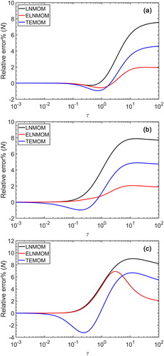
Figure 2 shows the relative error of $N$ for the LNMOM, the ELNMOM and the TEMOM for different initial cases in the continuum regime. For ${\sigma }_0$=1.1, the three error curves initially become slightly negative and then increase in the positive direction. Although the relative error of $N$ for the ELNMOM is initially larger than that of the LNMOM and the TEMOM, this error is very small compared with the maximum error. Table 3 shows the maximum relative error of $N$ for the LNMOM, the ELNMOM and the TEMOM for different initial cases. The maximum relative error for the ELNMOM at ${\sigma }_0$=1.1 is 1.42%, which is much smaller than 3.01% for the LNMOM and 2.70% for the TEMOM. For ${\sigma }_0$=1.4, the relative error of $N$ for the ELNMOM is smaller than that of the LNMOM and the TEMOM over the entire coagulation time. The maximum relative error for the ELNMOM is 1.60%. For ${\sigma }_0$=1.7, the TEMOM fails to predict the moment evolutions due to the limitation of the TEMOM ODEs (Yu et al. 2015). The relative error of $N$ for the ELNMOM is slightly smaller than that of the LNMOM in the intermediate stage. With ongoing coagulation, the relative error for the ELNMOM decreases faster and is much smaller than that of the LNMOM at $\tau =100$. Thus, the advantage of the ELNMOM over the LNMOM in predicting $N$ is not obvious in the intermediate stage for large ${\sigma }_0$. These comparisons indicate that the ELNMOM has higher accuracy in predicting the total particle number concentration than the LNMOM and the TEMOM over a wide range of initial conditions.

Figure 2. Relative error of $N$ for the LNMOM, the ELNMOM and the TEMOM for different initial cases in the continuum regime: (a) ${\sigma }_0$=1.1; (b) ${\sigma }_0$=1.4; (c) ${\sigma }_0$=1.7.

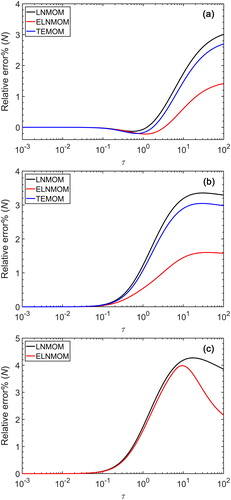
Table 3. Maximum relative error of $N$ for the LNMOM, the ELNMOM and the TEMOM for different initial cases in the continuum regime and the free-molecular regime.

Method	RE (continuum)			RE (free-molecular)
	${\sigma }_0$=1.1	${\sigma }_0$=1.4	${\sigma }_0$=1.7	${\sigma }_0$=1.1	${\sigma }_0$=1.4	${\sigma }_0$=1.7
LNMOM	3.01%	3.35%	4.27%	7.55%	7.89%	9.02%
ELNMOM	1.42%	1.60%	3.99%	1.97%	2.06%	6.90%
TEMOM	2.70%	3.05%	--	4.59%	4.89%	6.69%

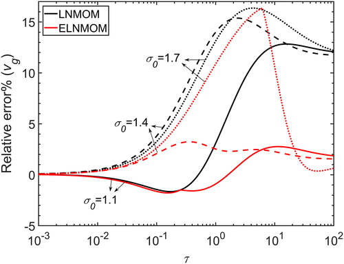
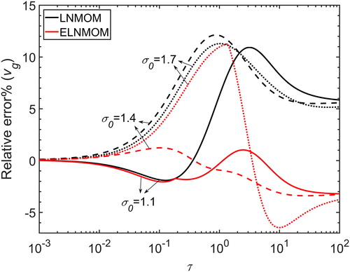
Figure 3 shows the relative error of $v_g$ for the LNMOM and the ELNMOM for different initial cases in the continuum regime. The calculation of $v_g$ is based on Equation (8)(8) $$v_g=M_1^2/\left(M_0^{3/2}{M}_2^{1/2}\right).$$(8) for the LNMOM and Equation (13)(13) $$v_g=\sqrt{v_{g1}{v}_{g2}}.$$(13) for the ELNMOM. The TEMOM is not included because it is unable to predict $v_g$ without an assumed form for the size distribution. For ${\sigma }_0$=1.1 and 1.4, the relative error of $v_g$ for the ELNMOM is much smaller than that of the LNMOM. The maximum relative error is 3.24% for the ELNMOM and 15.4% for the LNMOM. For ${\sigma }_0$=1.7, the relative error of $v_g$ for the ELNMOM is slightly smaller than that of the LNMOM in the intermediate stage. With ongoing coagulation, this error decreases dramatically and is less than 1% at $\tau =100$. For all initial cases, the ELNMOM more accurately predicts the geometric mean particle volume than the LNMOM.

Figure 3. Relative error of $v_g$ for the LNMOM and the ELNMOM for different initial cases in the continuum regime.

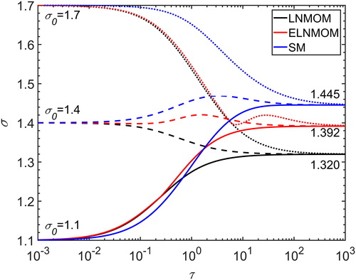
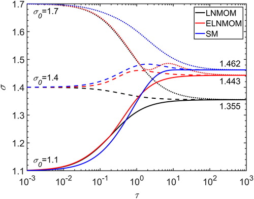
The size distribution will reach a self-preserving form for Brownian coagulation in the continuum regime (Friedlander 2000), which indicates that $\sigma$ will approach an asymptotic value in the long time limit. The asymptotic behavior is important for exploring the coagulation mechanism. Thus, the asymptotic $\sigma$ predicted by the LNMOM, the ELNMOM and the SM are compared here. The calculation of $\sigma$ is based on Equation (7)(7) $$\sigma =\hspace{0.17em}\text{exp}[\sqrt{\hspace{0.17em}\text{ln}\hspace{0.17em}(M_0{M}_2/M_1^2)}/3],$$(7) for the LNMOM and Equation (12)(12) $$\sigma =\hspace{0.17em}\text{exp}\hspace{0.17em}(\sqrt{{\hspace{0.17em}\text{ln}\hspace{0.17em}}^2(v_{g1}/v_{g2})/4+9{\hspace{0.17em}\text{ln}\hspace{0.17em}}^2{\sigma }^{\prime }}/3),$$(12) for the ELNMOM. For the SM, we use Equation (B21) from Landgrebe and Pratsinis (1990) to calculate $\sigma$. The total dimensionless coagulation time is set to 1000 to investigate the asymptotic behavior.

Figure 4 shows the variations of $\sigma$ with time for different initial ${\sigma }_0$ predicted by the LNMOM, the ELNMOM and the SM in the continuum regime. In all cases, $\sigma$ tends to the asymptotic value regardless of the initial ${\sigma }_0$, which agrees with the self-preserving size distribution in the continuum regime. The asymptotic $\sigma$ is 1.320 for the LNMOM and 1.392 for the ELNMOM. The asymptotic value of 1.320 for the LNMOM is the same as the result of Lee (1983). The accurate asymptotic $\sigma$ given by the SM is 1.445, which is the same as the result of Vemury and Pratsinis (1995). Thus, the asymptotic $\sigma$ predicted by the ELNMOM is much closer to the accurate result than that predicted by the LNMOM. Besides the asymptotic values of $\sigma$, the variation tendencies also differ for the three methods. The accurate results of the SM show that $\sigma$ initially increases and then decreases for ${\sigma }_0$=1.4. This non-monotonic variation of $\sigma$ is also observed in the predictions of the ELNMOM. However, the results of the LNMOM only show monotonic variations of $\sigma$.

Figure 4. Variations of $\sigma$ with time for different initial ${\sigma }_0$ predicted by the LNMOM, the ELNMOM and the SM in the continuum regime.

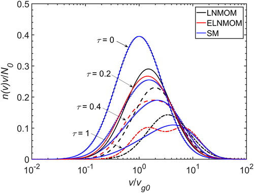
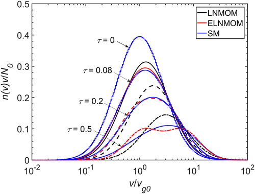
The extended size distribution is investigated by comparing the time evolution of the particle size distribution predicted by the LNMOM, the ELNMOM and the SM for ${\sigma }_0$=1.4, as shown in Figure 5. The SM gives accurate predictions for the actual size distribution. The LNMOM predicts a narrower size distribution than the SM at $\tau$=0.2, 0.4 and 1, which is mainly due to the log-normal distribution form of this method. The size distribution predicted by the ELNMOM is wider and much closer to the actual size distribution than that predicted by the LNMOM at $\tau$=0.2 and 0.4. However, the two subdistributions gradually separate and form a bimodal distribution at $\tau$=1. This is because the present ELNMOM assumes the same $N$ and $\sigma$ for the subdistributions. With this restriction, the extended size distribution has to transform from a unimodal distribution to a bimodal distribution to satisfy the moments. Despite this problem, the size distribution parameters are all better predicted by the ELNMOM than by the LNMOM for Brownian coagulation in the continuum regime over the entire coagulation time.

Figure 5. Time evolution of the particle size distribution predicted by the LNMOM, the ELNMOM and the SM for ${\sigma }_0$=1.4 in the continuum regime.

3.2. Validation of the ELNMOM for Brownian coagulation in the free-molecular regime

The validation of the ELNMOM for Brownian coagulation in the free-molecular regime follows the same procedure as in the continuum regime. The dimensionless time is defined as $\tau =K_{fm}{N}_0{v}_{g0}^{1/6}t$. In dimensionless time units, the results are independent of $K_{fm}$, so $K_{fm}$=1 is used for simplicity. The total dimensionless coagulation time is 100.

Figure 6 shows the relative error of $N$ for the LNMOM, the ELNMOM and the TEMOM for different initial cases in the free-molecular regime. For ${\sigma }_0$=1.1 and 1.4, the ELNMOM clearly has the best accuracy in predicting $N$. The maximum relative error of $N$ for the ELNMOM is 1.97% at ${\sigma }_0$=1.1 and 2.06% at ${\sigma }_0$=1.4, as shown in Table 3. Thus, the ELNMOM can well predict the particle number trajectory for small ${\sigma }_0$. For ${\sigma }_0$=1.7, the relative error of $N$ for the ELNMOM is approximately the same as that of the LNMOM in the initial stage. With ongoing coagulation, the relative error for the ELNMOM decreases greatly and is much smaller than that of the LNMOM at $\tau$=100. These comparisons show that the ELNMOM is more accurate than the LNMOM and the TEMOM in predicting the total particle number concentration in the free-molecular regime.

Figure 6. Relative error of $N$ for the LNMOM, the ELNMOM and the TEMOM for different initial cases in the free-molecular regime: (a) ${\sigma }_0$=1.1; (b) ${\sigma }_0$=1.4; (c) ${\sigma }_0$=1.7.

Figure 7 shows the relative error of $v_g$ for the LNMOM and the ELNMOM for different initial cases in the free-molecular regime. For ${\sigma }_0$=1.1 and 1.4, the maximum relative error for the ELNMOM is 3.40%, which is much smaller than 12.1% for the LNMOM. Thus, the time evolution of $v_g$ is well predicted by the ELNMOM for ${\sigma }_0$=1.1 and 1.4. For ${\sigma }_0$=1.7, the result is similar to that in the continuum regime. The advantage of the ELNMOM over the LNMOM is not obvious in this case. In general, the ELNMOM has higher accuracy in predicting the geometric mean particle volume than the LNMOM.

Figure 7. Relative error of $v_g$ for the LNMOM and the ELNMOM for different initial cases in the free-molecular regime.

The size distribution will also reach a self-preserving form in the free-molecular regime (Friedlander 2000). Previous studies have shown that the accurate asymptotic $\sigma$ is 1.462 in the free-molecular regime (Vemury and Pratsinis 1995). Figure 8 shows the variations of $\sigma$ with time for different initial ${\sigma }_0$ predicted by the LNMOM, the ELNMOM and the SM in the free-molecular regime. In all cases, $\sigma$ tends to the asymptotic value regardless of the initial ${\sigma }_0$, which agrees with the self-preserving size distribution in the free-molecular regime. The SM gives the accurate prediction of 1.462 for the asymptotic $\sigma$. The asymptotic $\sigma$ predicted by the LNMOM is 1.355, which agrees with the result of Lee, Chen, and Gieseke (1984). For the ELNMOM, the asymptotic $\sigma$ is 1.443, which is close to the accurate value. Thus, the ELNMOM more accurately describes the asymptotic behavior than the LNMOM in the free-molecular regime. The variations of $\sigma$ in the free-molecular regime are similar to those in the continuum regime. The LNMOM only gives monotonic predictions for the variations of $\sigma$ while the ELNMOM can track the non-monotonic variations of $\sigma$.

Figure 8. Variations of $\sigma$ with time for different initial ${\sigma }_0$ predicted by the LNMOM, the ELNMOM and the SM in the free-molecular regime.

Figure 9 shows the time evolution of the particle size distribution predicted by the LNMOM, the ELNMOM and the SM for ${\sigma }_0$=1.4 in the free-molecular regime. The results are similar to those in the continuum regime. In the initial stage, the size distribution predicted by the ELNMOM is wider and much closer to the actual size distribution than that predicted by the LNMOM. As coagulation proceeds, a bimodal distribution is observed in the predictions of the ELNMOM. The explanations for this result are the same as those in Section 3.1. Despite this problem, the ELNMOM gives better predictions on all the size distribution parameters than the LNMOM for Brownian coagulation in the free-molecular regime over the entire coagulation time.

Figure 9. Time evolution of the particle size distribution predicted by the LNMOM, the ELNMOM and the SM for ${\sigma }_0$=1.4 in the free-molecular regime.

3.3. Computational efficiency

The ELNMOM has an additional moment equation to solve as compared with the LNMOM. Moreover, the moment conversion of the ELNMOM is more complex. Thus, the computational cost of the ELNMOM should be larger than that of the LNMOM. Therefore, we need to evaluate the computational efficiency of the ELNMOM. The total dimensionless coagulation time is set to 100 and the tolerances of the ODE solver are kept the same for different methods. The computation time is found to change little for different initial ${\sigma }_0$. Thus, ${\sigma }_0$=1.4 is used as a representative initial condition.

Table 4 shows the computation time in seconds for the LNMOM, the ELNMOM and the TEMOM for ${\sigma }_0$=1.4 in the continuum regime and the free-molecular regime. The results show that the TEMOM has the highest computational efficiency. The reason is that the TEMOM only includes three first-order ODEs and has no moment conversion. As a comparison, the solution procedures of the LNMOM and the ELNMOM include intermediate moment conversions. The computation time of the ELNMOM is about 1.6 times that of the LNMOM, which is acceptable since the LNMOM is already a highly efficient method. Thus, the ELNMOM is also an efficient numerical method.

Table 4. Computation time for the LNMOM, the ELNMOM and the TEMOM for ${\sigma }_0$=1.4 in the continuum regime and the free-molecular regime.

Method	Time (continuum)	Time (free-molecular)
LNMOM	0.114s	0.146s
ELNMOM	0.177s	0.244s
TEMOM	0.050s	0.064s

4. Conclusions

In this study, we developed the ELNMOM as an extension to the conventional LNMOM for solving the PBE for Brownian coagulation. The ELNMOM uses the superposition of log-normal subdistributions to represent the size distribution. Unlike previous modal studies, the subdistributions are not physically distinguished as different modes and the closure is achieved through introducing additional higher-order moment equations. The simplest version of the ELNMOM with four adjustable parameters was implemented for a preliminary exploration.

The four-parameter ELNMOM was validated by comparing the predicted size distribution parameters with those predicted by the LNMOM and other numerical methods for Brownian coagulation in the continuum regime and the free-molecular regime. Three different initial cases (${\sigma }_0$=1.1, 1.4 and 1.7) were selected to represent monodispersed to polydispersed aerosols. The results show that the ELNMOM more accurately predicts the time evolution of $N$, $\sigma$ and $v_g$ than the LNMOM over the entire coagulation time. Especially for ${\sigma }_0$=1.1 and 1.4, the accuracy is much better than that of the LNMOM. In addition, the ELNMOM does not take much more computation time than the LNMOM. Thus, the ELNMOM is verified as an efficient and useful tool for predicting the size distribution parameters for Brownian coagulation. As for the actual size distribution, the ELNMOM gives better predictions than the LNMOM in the initial stage. However, the long-time size distribution cannot be well described by this method. Generally, the actual size distribution is much more difficult to predict than the moments. The limitation of the present method is due to the assumption of the same $N$ and $\sigma$ for the two subdistributions. Future research will focus on removing the assumption on $N$ and $\sigma$ to resolve the current limitation.

Nomenclature
$b_k$	=	correction factor
$k_B$	=	boltzmann constant, J/K
$K_{co}$	=	collision coefficient for the continuum regime
$K_{fm}$	=	collision coefficient for the free-molecular regime
$M_k$	=	kth moment of the particle size distribution
$N$	=	total particle number concentration, m-3
$n$	=	particle number concentration density
$P$	=	size distribution parameter
$T$	=	gas temperature, K
$t$	=	time, s
$v$	=	particle volume, m3
$v_g$	=	geometric number mean particle volume, m3

Greek letters
$\beta$	=	collision kernel
$\sigma$	=	geometric standard deviation based on the particle diameter
$\mu$	=	gas viscosity, kg/m/s
${\rho }_p$	=	particle density, kg/m3
$\tau$	=	dimensionless time

Abbreviations
ELNMOM	=	extended log-normal method of moments
FEM	=	finite element method
LNMOM	=	log-normal method of moments
MAD	=	modal aerosol dynamics
MOM	=	method of moments
ODE	=	ordinary differential equation
PBE	=	population balance equation
RE	=	relative error
SM	=	sectional method
TEMOM	=	Taylor series expansion method of moments

Disclosure statement

No potential conflict of interests was reported by the authors.

Additional information

Funding

This work was supported by the National Key R&D Program of China [grant number 2016YFC0202700], the National Natural Science Foundation of China [grant number 51676112] and State Environmental Protection Key Laboratory of Sources and Control of Air Pollution Complex.

References

- Barrett, J. C., and J. S. Jheeta. 1996. Improving the accuracy of the moments method for solving the aerosol general dynamic equation. J. Aerosol Sci. 27 (8):1135–1142. doi: 10.1016/0021-8502(96)00059-6.
- Barrett, J. C., and N. A. Webb. 1998. A comparison of some approximate methods for solving the aerosol general dynamic equation. J. Aerosol Sci. 29 (1–2):31–39. doi: 10.1016/S0021-8502(97)00455-2.
- Diemer, R. B., and J. H. Olson. 2002. A moment methodology for coagulation and breakage problems: Part 2 – moment models and distribution reconstruction. Chem. Eng. Sci. 57 (12):2211–2228. doi: 10.1016/S0009-2509(02)00112-4.
- Frenklach, M. 2002. Method of moments with interpolative closure. Chem. Eng. Sci. 57 (12):2229–2239. doi: 10.1016/S0009-2509(02)00113-6.
- Frenklach, M., and S. J. Harris. 1987. Aerosol dynamics modeling using the method of moments. J. Colloid Interf. Sci. 118 (1):252–261. doi: 10.1016/0021-9797(87)90454-1.
- Friedlander, S. K. 2000. Smoke, dust, and haze: Fundamentals of aerosol dynamics. New York; Oxford: Oxford University Press.
- Gelbard, F., Y. Tambour, and J. H. Seinfeld. 1980. Sectional representations for simulating aerosol dynamics. J. Colloid Interf. Sci. 76 (2):541–556. doi: 10.1016/0021-9797(80)90394-X.
- Jeong, J. I., and M. Choi. 2004. A bimodal moment model for the simulation of particle growth. J. Aerosol Sci. 35 (9):1071–1090. doi: 10.1016/j.jaerosci.2004.04.005.
- John, V., I. Angelov, A. A. Oncul, and D. Thevenin. 2007. Techniques for the reconstruction of a distribution from a finite number of its moments. Chem. Eng. Sci. 62 (11):2890–2904. doi: 10.1016/j.ces.2007.02.041.
- Kajino, M. 2011. MADMS: Modal aerosol dynamics model for multiple modes and fractal shapes in the free-molecular and near-continuum regimes. J. Aerosol Sci. 42 (4):224–248. doi: 10.1016/j.jaerosci.2011.01.005.
- Kruis, F. E., A. Maisels, and H. Fissan. 2000. Direct simulation Monte Carlo method for particle coagulation and aggregation. AIChE J. 46 (9):1735–1742. doi: 10.1002/aic.690460905.
- Kumar, J., M. Peglow, G. Warnecke, S. Heinrich, and L. Morl. 2006. Improved accuracy and convergence of discretized population balance for aggregation: The cell average technique. Chem. Eng. Sci. 61 (10):3327–3342. doi: 10.1016/j.ces.2005.12.014.
- Landgrebe, J. D., and S. E. Pratsinis. 1990. A discrete-sectional model for particulate production by gas-phase chemical-reaction and aerosol coagulation in the free-molecular regime. J. Colloid Interf. Sci. 139 (1):63–86. doi: 10.1016/0021-9797(90)90445-T.
- Lee, K. W. 1983. Change of particle-size distribution during Brownian coagulation. J. Colloid Interf. Sci. 92 (2):315–325. doi: 10.1016/0021-9797(83)90153-4.
- Lee, K. W., H. Chen, and J. A. Gieseke. 1984. Log-normally preserving size distribution for Brownian coagulation in the free-molecule regime. Aerosol Sci. Technol. 3 (1):53–62. doi: 10.1080/02786828408958993.
- Lee, K. W., and J. Hwang. 1997. Erratum to “log-normally preserving size distribution for Brownian coagulation in the free molecule regime” by Lee et al. and “coagulation rate of polydisperse particles” by Lee and Chen. Aerosol Sci. Technol. 26 (5):469–470. doi: 10.1080/02786829708965446.
- Mann, G. W., K. S. Carslaw, D. V. Spracklen, D. A. Ridley, P. T. Manktelow, M. P. Chipperfield, S. J. Pickering, and C. E. Johnson. 2010. Description and evaluation of GLOMAP-mode: A modal global aerosol microphysics model for the UKCA composition-climate model. Geosci. Model Dev. 3 (2):519–551. doi: 10.5194/gmd-3-519-2010.
- Marchisio, D. L., and R. O. Fox. 2005. Solution of population balance equations using the direct quadrature method of moments. J. Aerosol Sci. 36 (1):43–73. doi: 10.1016/j.jaerosci.2004.07.009.
- McGraw, R. 1997. Description of aerosol dynamics by the quadrature method of moments. Aerosol Sci. Technol. 27 (2):255–265. doi: 10.1080/02786829708965471.
- Megaridis, C. M., and R. A. Dobbins. 1990. A bimodal integral solution of the dynamic equation for an aerosol undergoing simultaneous particle inception and coagulation. Aerosol Sci. Technol. 12 (2):240–255. doi: 10.1080/02786829008959343.
- Müller, H. 1928. Zur allgemeinen theorie ser raschen koagulation. Fortschrittsber. Kolloide Polym. 27:223–250. doi: 10.1007/BF02558510.
- Otto, E., H. Fissan, S. H. Park, and K. W. Lee. 1997. Brownian coagulation in the transition regime using the moments of a lognormal distribution. J. Aerosol Sci. 28:S629–S630. doi: 10.1016/S0021-8502(97)85314-1.
- Otto, E., H. Fissan, S. H. Park, and K. W. Lee. 1999. The log-normal size distribution theory of Brownian aerosol coagulation for the entire particle size range: Part II – Analytical solution using Dahneke's coagulation kernel. J. Aerosol Sci. 30 (1):17–34. doi: 10.1016/S0021-8502(98)00038-X.
- Palaniswaamy, G., and S. K. Loyalka. 2008. Direct simulation, Monte Carlo, aerosol dynamics: Coagulation and condensation. Ann. Nucl. Energ. 35 (3):485–494. doi: 10.1016/j.anucene.2007.06.024.
- Park, S. H., and K. W. Lee. 2002. Change in particle size distribution of fractal agglomerates during Brownian coagulation in the free-molecule regime. J. Colloid Interf. Sci. 246 (1):85–91. doi: 10.1006/jcis.2001.7946.
- Park, S. H., R. Xiang, and K. W. Lee. 2000. Brownian coagulation of fractal agglomerates: Analytical solution using the log-normal size distribution assumption. J. Colloid Interf. Sci. 231 (1):129–135. doi: 10.1006/jcis.2000.7102.
- Pratsinis, S. E. 1988. Simultaneous nucleation, condensation, and coagulation in aerosol reactors. J. Colloid Interf. Sci. 124 (2):416–427. doi: 10.1016/0021-9797(88)90180-4.
- Ramkrishna, D., and M. R. Singh. 2014. Population balance modeling: Current status and future prospects. Ann. Rev. Chem. Biomol. 5 (1):123–146. doi: 10.1146/annurev-chembioeng-060713-040241.
- Seo, Y., and J. R. Brock. 1990. Distributions for moment simulation of aerosol evaporation. J. Aerosol Sci. 21 (4):511–514. doi: 10.1016/0021-8502(90)90127-J.
- Shekar, S., A. J. Smith, W. J. Menz, M. Sander, and M. Kraft. 2012. A multidimensional population balance model to describe the aerosol synthesis of silica nanoparticles. J. Aerosol Sci. 44:83–98. doi: 10.1016/j.jaerosci.2011.09.004.
- Smoluchowski, M. V. 1918. Versuch einer mathematischen theorie der koagulationskinetik kolloider lösungen. Z. Phys. Chem. 92:129–168.
- Vemury, S., and S. E. Pratsinis. 1995. Self-preserving size distributions of agglomerates. J. Aerosol Sci. 26 (2):175–185. doi: 10.1016/0021-8502(94)00103-6.
- Wang, K., W. Peng, and S. Yu. 2019. A new approximation approach for analytically solving the population balance equation due to thermophoretic coagulation. J. Aerosol Sci. 128:125–137. doi: 10.1016/j.jaerosci.2018.11.010.
- Whitby, E. R., and P. H. McMurry. 1997. Modal aerosol dynamics modeling. Aerosol Sci. Technol. 27 (6):673–688. doi: 10.1080/02786829708965504.
- Xie, M. L., and Q. He. 2013. Analytical solution of temom model for particle population balance equation due to Brownian coagulation. J. Aerosol Sci. 66:24–30. doi: 10.1016/j.jaerosci.2013.08.006.
- Yamamoto, M. 2004. A moment method of an extended log-normal size distribution application to Brownian aerosol coagulation. J. Aerosol Res. 19:41–49.
- Yu, M. Z., and J. Z. Lin. 2009. Solution of the agglomerate Brownian coagulation using Taylor-expansion moment method. J. Colloid Interf. Sci. 336 (1):142–149. doi: 10.1016/j.jcis.2009.03.030.
- Yu, M. Z., J. Z. Lin, and T. L. Chan. 2008. A new moment method for solving the coagulation equation for particles in Brownian motion. Aerosol Sci. Technol. 42 (9):705–713. doi: 10.1080/02786820802232972.
- Yu, M. Z., and T. L. Chan. 2015. A bimodal moment method model for submicron fractal-like agglomerates undergoing Brownian coagulation. J. Aerosol Sci. 88:19–34. doi: 10.1016/j.jaerosci.2015.05.011.
- Yu, M. Z., X. T. Zhang, G. D. Jin, J. Z. Lin, and M. Seipenbusch. 2015. A new analytical solution for solving the population balance equation in the continuum-slip regime. J. Aerosol Sci. 80:1–10. doi: 10.1016/j.jaerosci.2014.10.007.
- Zhao, H. B., and C. G. Zheng. 2013. A population balance-Monte Carlo method for particle coagulation in spatially inhomogeneous systems. Comput. Fluids 71:196–207. doi: 10.1016/j.compfluid.2012.09.025.