Combining sensor-based measurement and modeling of PM_2.5 and black carbon in assessing exposure to indoor aerosols

Abstract

Accurate, cost-effective methods are needed for rapid assessment of traffic-related air pollution (TRAP). Typically, real-time data of particulate matter (PM) from portable sensors have been adjusted using data from reference methods such as gravimetric measurement to improve accuracy. The objective of this study was to create a correction factor or linear regression model for the real-time measurements of the RTI’s Micro Personal Exposure Monitor (MicroPEM™) and AethLab’s microAeth^® black carbon (AE51) sensor to generate accurate real-time data for PM_2.5 (PM_2.5RT) and black carbon (BC_RT) in Cincinnati metropolitan homes. The two sensors and an SKC PM_2.5 Personal Modular impactor were collocated in 44 indoor sampling events for 2 days in residences near major roadways. The reference filter-based analyses conducted by a laboratory included particle mass (SKC PM_2.5 and MicroPEM™ PM_2.5) and black carbon (SKC BC); these methods are more accurate than real-time sensors but are also more cumbersome and costly. For PM_2.5, the average correction factor, a ratio of gravimetric to real time, for the MicroPEM™ PM_2.5 and SKC PM_2.5 utilizing the PM_2.5RT and was 0.94 and 0.83, respectively, with a coefficient of variation (CV) of 84% and 52%, respectively; the corresponding linear regression model had a CV of 54% and 25%. For BC, the average correction factor utilizing the BC_RT and SKC BC was 0.74 with a CV of 36% with the associated linear regression model producing a CV of 56%. The results from this study will help ensure that the real-time exposure monitors are capable of detecting an estimated PM_2.5 after an appropriate statistical model is applied.

Copyright © 2019 American Association for Aerosol Research

EDITOR:

• Pramod Kulkarni

1. Introduction

Traffic pollutants include a mixture of particulate matter (PM), black carbon (BC), nitrogen dioxide, carbon monoxide, volatile organic compounds, and nitrogen oxides. Vehicle exhaust emissions formed by fuel combustion in the engine typically fall within the size range of particulate matter less than 2.5 µm (PM_2.5) (Jamriska, Morawska and Mergersen 2008). In 2018, the Cincinnati metropolitan area was 18th among the 25 U.S. cities most polluted by year-round particle pollution (annual PM_2.5) (Billings et al. 2018). Motor vehicle traffic has been determined to be a major source for U.S. PM_2.5 (Thurston, Ito and Lall 2011). The generic term BC refers to particles formed through incomplete combustion of fossil fuels, biofuels, or biomass, and has evolved over time to include combustion byproducts. Black carbon or “soot carbon” are often used interchangeably for the light-absorbing component of combustion aerosols (Andreae and Gelencsér 2006). Soot carbon is often referred to as an impure form of near-elemental carbon, and it typically includes proportions of other atoms, such as polycyclic aromatic hydrocarbons. The strong light absorption of carbon aerosols allows them to be detected by a multi-wavelength optical absorption technique to measure BC (Yan et al. 2011).

Particles associated with traffic-related air pollution (TRAP) penetrate homes and occupational settings, affecting the indoor air quality (Jung et al. 2010; Martuzevicius et al. 2008). It has been estimated that 30%–45% of people in large North American cities reside within 300 to 500 meters from a major road, and exposures to traffic-related pollution are likely to be of public health concern (Health Effects Institute 2010). In addition, people spend approximately 87% of their time in enclosed buildings in the United States (Klepeis et al. 2001). The quality of indoor air will vary depending on the tightness of the building, indoor emissions (such as cooking, candle/incense, mold, chemicals), filtration systems and settings in the building, and distance from traffic or pollution sources (Stephens and Siegel 2012a). Exposure to TRAP aerosols has been linked with reduced respiratory health in both public and worker populations (Gehring et al. 2010; Health Effects Institute 2010; Ryan et al. 2009; Volpino et al. 2004). A review by Grahame et al. (2014) showed that BC from various sources appears to be causally involved in cardiovascular mortality, morbidity, and perhaps adverse birth and nervous system effects. The particles associated with TRAP can penetrate the home or office indoor environment, where people spend a majority of their time, thus leading to these above-listed and other poor health outcomes (Bernstein et al. 2008; The National Academies of Sciences Engineering and Medicine 2016).

Better methods are needed for inexpensive and accurate assessment of population exposure to traffic-related aerosols so that full characterizations of potential health effects can be made. The inability to attribute measurable ambient air concentrations to personal exposure is a major limitation of understanding the potential health effects of air pollutants (Bernstein et al. 2008). Studies have shown that personal exposures to PM_2.5 could be 1.4 times as high as the indoor concentration as measured by a stationary monitor; therefore, accurate assessment of personal exposure should include the breathing zone (Ferro, Kopperud and Hildemann 2004). The National Research Council strongly supports the application of personal exposure monitors (PEMs) to characterize exposure levels and patterns for correlation with acute- and chronic-scale health effects (National Research Council 2004). In order to make characterizations concerning health effects associated with TRAP exposure, these instruments need to be accurate and precise. Individuals generally do not prefer wearing noisy and bulky personal samplers; they may not wear these at all or wear them incorrectly. MicroPEM™ (RTI International, Raleigh, NC, USA) and microAeth^® (AE51; AethLabs San Francisco, CA, USA) are real-time aerosol sensors that are compact, low cost and could allow for a large-scale air quality study that is typically unattainable when performing costly and cumbersome filter analyses. Both devices are quiet, self-contained instruments with built-in pumps, flow control, data storage, battery, and a sensor for temperature. The real-time measurements from the MicroPEM™ and the microAeth^® are based on detecting a mixture of ambient particles with differing composition and size distributions resulting in differing optical properties, which can lead to potential error and uncertainty.

The MicroPEM™ provides personal simultaneous measurements of PM_2.5 with both the integrated exposure (from filter-based measurements) and the patterns of exposure (from real-time measurements). The onboard 3-axis accelerometer monitors the frequency and intensity of movement and can be combined with PM_2.5 concentration to calculate the potential inhaled dose (Cho et al. 2016). The MicroPEM™ has been used in numerous studies including personal air pollutant exposures in inner-city asthmatic children (Dutmer et al. 2015), mold contamination in schools with either high or low prevalence of asthma (Vesper et al. 2015) and personal and fixed-location PM_2.5 continuous exposure monitoring (Cho et al. 2016; Sloan et al. 2016). The MicroPEM™ nephelometer detects particles by transforming the intensity of scattered laser light into particle mass. The optical properties and sizes of PM affect the degree of light scattering and can introduce potential error for real-time mass concentration measurements. Typically, the real-time data are adjusted with the gravimetrically measured filter-based PM_2.5 to account for these errors. By determining a correction factor (CF) or regression model for the MicroPEM™, the real-time data would serve as a useful source for determining exposure to PM_2.5 while saving the time and effort associated with filter analysis and adjustment.

The microAeth^® sensor is a compact, real-time, wearable BC monitor designed for on-person, mobile applications. The microAeth^® real-time data on black carbon (BC_RT), however, does not typically rely on a filter-based BC adjustment, and is used widely in BC studies such as: exposure to ultrafine particles and BC in diesel-powered commuter trains (Jeong, Traub and Evans 2017), TRAP exposure in designing urban bicycle networks (Minet et al. 2018), and personal exposure to BC on changes in allergic asthma gene methylation (Jung et al. 2017). The microAeth^® BC sensor continuously collects aerosol particles onto a filter and an optical detector measures the rate of change of attenuation due to the absorbance of transmitted light by particles that are being collected. The measurement at 880 nm is interpreted as the concentration of BC. The particles in the filter matrix can cause scattering effects which may result in errors in BC determination if scattered light is wrongly attributed to absorption (Ballach et al. 2001). An alternative method to the microAeth^® is to analyze filters for BC optically in a laboratory setting; however, this method would be more cumbersome, expensive, and time-consuming. The laboratory filter-based analysis could utilize a single wavelength or a multi-wavelength optical absorption technique with an integrative-sphere that uses a gravimetric standard. To prevent matrix effects from filter materials, an interface between the filter and integrating sphere minimizes light loss, and increases the sensitivity and reliability (Yan et al. 2011). Utilizing the laboratory filter-based analysis as a more accurate approach, a CF or regression model could be developed to improve BC_RT accuracy.

The goal of this study was to develop CFs and models to improve the accuracy of the MicroPEM™ PM_2.5 and the microAeth^® BC sensors for real-time monitoring and to eliminate the extra time and cost associated with filter analysis. Two real-time sensors and a traditional filter sample were deployed in high traffic-impacted homes to develop a CF or linear regression model that would allow for eliminating the need for filter analysis. Home characteristics and sampling conditions were included in the linear regression models. The limitations of the real-time monitoring can be overcome by utilizing a regression model or CF developed by comparing data from these instruments with a more accurate filter method.

2. Methods

2.1. Sampling conditions

In conjunction with an ongoing study aimed at assessing the effectiveness of a portable air cleaner utilizing high-efficiency particle air (HEPA) filtration in removing traffic-related aerosol particles (Cox et al. 2018), sampling was performed in bedrooms of asthmatic children from October of 2015 to May of 2017. Study subjects were recruited from the Asthma Center at the Cincinnati Children’s Hospital Medical Center and participants of the Cincinnati Childhood Allergy and Air Pollution Study (CCAAPS) (LeMasters et al. 2006). Children (age 10–15) with asthma were considered eligible for the study if their primary residence was <500 meters from a major roadway (Health Effects Institute 2010) or if the home had an elevated concentration of elemental carbon (EC). The latter was estimated using a previously validated land-use regression model, which takes into account many factors including wind direction, length of bus routes, a measure of truck intensity, and elevation (Ryan et al. 2008). The primary output from the land-use regression model is the EC attributable to traffic (ECAT); ECAT values ≥0.32 µg/m³ were considered elevated. State highways or federal interstates with an average daily truck count of more than 1000 were defined as major roads. Locations of state highways, federal interstates, and the average daily truck counts on each road were obtained from the Ohio Department of Transportation.

Using a checklist, the research team recorded observations regarding the characteristics of the study homes including age and type of buildings, its size, presence of smokers in the home, and the presence of dogs or cats. Conditions during sampling such as season, kitchen fan, frying food, candle burning, cleaning activities, and opening windows were recorded based on the recollection of participants during the sampling time (48 h). Winter was considered January through March, spring was considered April through June, summer was considered July through September, and fall was considered October through December. This study required and received approval from the Institutional Review Board of the University of Cincinnati.

2.2. Sample collection and analysis

Sample collection for the current study was performed prior to any air cleaner treatment in the home. The MicroPEM™ sensors (RTI International, Research Triangle Park, NC, USA) with PM_2.5 inlets were loaded with pre-weighed 25-mm diameter and 3-µm pore size polytetrafluoroethylene (PTFE) filters with a polymethylpentene (PMP) ring (Zefon, Ocala, FL, USA) and were deployed at a flow rate of 0.5 L/min. Personal Modular PM_2.5 impactors (SKC Inc., Eighty-four, PA, USA) with a pre-weighed 37-mm diameter and 2-µm pore size PTFE filters with a PMP ring (Pall, Port Washington, NY, USA) were deployed at 3 L/min. Both filters were analyzed gravimetrically for PM_2.5 (Zhang et al. 2017). The SKC filters were also analyzed for BC by a multi-wavelength optical absorption technique based on a gravimetric calibration (Yan et al. 2011). When generally discussing laboratory-based PM_2.5 or BC analyses, hereafter they will be called “filter-based.” The microAeth^® (AE51, AethLabs, San Francisco, CA, USA) air sample was collected on a filter strip consisting of PTFE-coated glass fiber that was discarded and replaced after each sample. The microAeth^® operated at a flow rate of 0.15 L/min.

MicroPEM™, microAeth^®, and SKC impactors were co-located for 48 h in 44 sampling events. Media and field blanks were collected in parallel of 10% of all samples. All filters were stored at −20 °C before analysis.

2.3. Data analysis

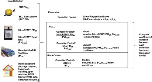
The PM_2.5 concentrations obtained with the MicroPEM™ filter (hereafter referred to as “MicroPEM™ PM_2.5”) (n = 33) and the SKC impactor (“SKC PM_2.5”) (n = 24) were compared with each other and with the 48-h average PM_2.5 calculated from the real-time data obtained with the MicroPEM™ (“PM_2.5RT”) (n = 36). The limit of detection of the MicroPEM™ PM_2.5RT nephelometer was 3 µg/m³; therefore, all readings below this value were not used. The MicroPEM™ PM_2.5RT data are typically adjusted using the simultaneous filter sampling value (MicroPEM™ PM_2.5). However, in this study the MicroPEM™ PM_2.5RT values were not gravimetrically adjusted per sample as the study aim was to develop CFs and regression models. The MicroPEM™ CF was calculated as the ratio of the PM_2.5 concentration obtained with the MicroPEM™ PM_2.5 and the PM_2.5RT (CF₁ = MicroPEM™ PM_2.5/PM_2.5RT). As comparison and validation, a CF based on SKC PM_2.5 results was also calculated and evaluated (CF₂ = SKC PM_2.5/PM_2.5RT) (Figure 1).

Figure 1. Flow chart describing study design.

The real-time data from the microAeth^® (“BC_RT”) were post-processed by the manufacturer utilizing an optimized noise reduction averaging (ONA) algorithm (Hagler et al. 2011). The incremental light attenuation through the instrument’s filter defined the time window of averaging; the ONA program performed adaptive time-averaging of the BC data. The maximum optical attenuation value was considered to be 80 (Good et al. 2017; Hansen 2005). The data were further processed by our team to correct for potential underestimation associated with increased BC mass on the filter (Apte et al. 2011; Good et al. 2017; Kirchstetter and Novakov 2007; Lin et al. 2017). The instrument-reported change in attenuation coefficient (ATN) was used in the correction as follows: (1) $$\text{BC} ={ \text{BC}}_0\times {(0.88(\hspace{0.17em}\text{exp}\hspace{0.17em}(-\text{ATN}/100))+0.12)}^{-1}$$(1) where BC is the corrected BC concentration and BC₀ is the instrument-reported concentration.

The BC concentration obtained with the SKC impactor (“SKC BC”) was compared with the BC_RT values averaged over 48 h (n = 23). The CF was calculated as the ratio between SKC BC concentration and BC_RT concentration (CF₃ = SKC BC/BC_RT).

2.4. Statistical analysis

R (version 3.1.1) was utilized for the statistical analysis (Ihaka and Gentleman 1996). A Wilcoxon signed-rank test and Spearman’s rank correlation coefficient were used to study differences and correlations, respectively. The analysis had three components: (1) Filter and real-time data were compared: SKC PM_2.5, MicroPEM™ PM_2.5, PM_2.5RT, the SKC BC and BC_RT, (2) the CFs (CF₁, CF₂, and CF₃) and corresponding coefficients of variation were calculated, and (3) the linear regression models incorporated the real-time sensor data and home characteristic variables, and based on those predictions, coefficients of variation were calculated (Figure 1).

In (3), to develop a corrective model for real-time data from the sensores, variable selection was performed by using the best subset regression test, and the final models were selected based on the lowest Akaike information criterion (AIC) (Clark et al. 2010; Jerrett et al. 2007). SKC PM_2.5, MicroPEM™ PM_2.5, and SKC BC values were natural log-transformed to improve normality. Prior to the selection of the final regression model, the independent variables available included age of building, type of flooring, ECAT concentration, the average daily truck count within 400 meters, distance to state highways, distance to a major road, and the presence of smokers, pets, or HEPA or electrostatic filter in the heating, ventilation and air conditioning (HVAC) system in the home. Furthermore, conditions during sampling such as open windows, operating kitchen fan, frying food, burning candles, and cleaning activities including vacuuming, dusting, or sweeping, were independent variables prior to variable selection for the final model. All variables selected by the best subset test which generated a model with the lowest AIC were included into the multiple linear regression models. Two regression models were developed for MicroPEM™ PM_2.5 and the SKC PM_2.5 using PM_2.5RT and the above mentioned independent variables. A third model was developed for SKC BC using BC_RT and independent variables (hereafter called “multiple regression models”). The coefficient of variation (CV) was calculated for each CF and for the predictions of the multiple regression models.

For comparison, simple linear regression models using PM_2.5RT with no additional independent variables were developed for MicroPEM™ PM_2.5 and the SKC PM_2.5, and a third simple linear regression model using BC_RT with no additional independent variables was developed for SKC BC. The data were randomly divided into two sets: 75% training set and 25% test set. Residual sum of squares (RSS) was calculated for the three simple models and the three multiple regression models. The predicted values obtained from the multiple and simple regression models were compared to the measured filter values for the MicroPEM™ PM_2.5, the SKC PM_2.5, and the SKC BC utilizing Spearman’s correlation coefficients and Wilcoxon signed-rank tests p-values.

When utilizing Spearman’s correlation coefficients or Wilcoxon signed-rank tests, a Bonferroni correction was used to adjust for multiple comparisons. Since three primary methods were evaluated at a time (PM_2.5RT, SKC PM_2.5, and the MicroPEM™ PM_2.5), p-values less than 0.0167 (0.05/3) were considered significant for multiple comparisons. For multiple and simple linear regression models, a value of p < 0.05 was considered significant.

2.5. NIOSH criterion

While there are no specific criteria for BC and PM_2.5 direct reading sensors, a guideline document from the National Institute for Occupational Safety and Health (NIOSH) sets forth a criterion for direct-reading gas and vapor sensors (NIOSH 2012). The accuracy criterion in this document requires that readings from a direct-reading monitor to be within ±25% of the true concentration, having a probability of 95% for an individual observation (i.e., that the accuracy of an acceptable monitor is no greater than 25%). For our purposes, the sensors and models 95% confidence interval (CI) of should fall within ±25% of the filter-based concentration to be used for both compliance and range finding monitoring.

Errors of the sensor readings and model predictions were calculated by finding the percent difference between the model predictions, or sensor value, and the reference (filter-based measurement values) (Equation (2)(2) $$\mathit{Error}=\left(\right(\mathit{Sensor}\mathrm{ }\mathit{value}\mathrm{ }\mathit{or}\mathrm{ }\mathit{Model}\mathrm{ }\mathit{prediction}-\mathit{Reference})/\mathit{Reference})\mathrm{*}100$$(2) ). As the data were not distributed normally and had a bias >10%, a bias-corrected bootstrap method was used to calculate 95% CI for the error (Wang 2001): (2) $$\mathit{Error}=\left(\right(\mathit{Sensor}\mathrm{ }\mathit{value}\mathrm{ }\mathit{or}\mathrm{ }\mathit{Model}\mathrm{ }\mathit{prediction}-\mathit{Reference})/\mathit{Reference})\mathrm{*}100$$(2)

3. Results

3.1. Study participants

There were 44 sampling events in 33 homes in which the MicroPEM™, the microAeth^®, and the SKC Impactor were deployed. Single-family homes accounted for 70% with the remaining being apartments or condominiums. The homes were built between 1865 and 2016. The average area of the home was 188 m², with the room being sampled having an average area of 15 m². Carpet was present in 61% of the sampled rooms with the remaining having hardwood, and 70% of the homes had cats and/or dogs (Table S1 in the online supplementary information [SI]). To explore the relationships between the PM_2.5 and BC concentrations and several of the home characteristics, scatter plots were developed and can be seen in Figure S1 in SI.

3.2. PM_2.5 and BC results

The PM_2.5 medians from the SKC PM_2.5, MicroPEM™ PM_2.5, and PM_2.5RT ranged from 7.5 to 11.2 µg/m³ and the means ranged from 12.7 to 16.3 µg/m³ (Table 1 and Figure 2a). There was a significant correlation (Spearman) between the SKC PM_2.5 and the MicroPEM™ PM_2.5 (r = 0.74, p < 0.001), between the SKC PM_2.5 and the average of PM_2.5RT (r = 0.77, p < 0.001), as well as between the MicroPEM™ PM_2.5 and the PM_2.5RT (r = 0.62, p < 0.001) (Table 2). Based on Wilcoxon test, the median of PM_2.5RT was significantly different from both gravimetric analyses, the median of MicroPEM™ PM_2.5 (p < 0.01, n = 33) and the median of the SKC PM_2.5 (p < 0.0167, n = 24). No significant difference was found between the two gravimetric analyses, MicroPEM™ PM_2.5 and the SKC PM_2.5 (p = 0.08, n = 21) (Figure 2).

Figure 2. (a) PM_2.5 values (µg/m³) obtained as MicroPEM™ real-time-averaged values (PM_2.5RT) (n = 36), SKC PM_2.5 (n = 24), MicroPEM™ PM_2.5 (n = 33). (b) Black carbon (BC) values (µg/m³) obtained as microAeth^® averaged real-time values of BC (BC_RT) and SKC BC (n = 23). Horizontal lines in the box plots represent the 10%, 25%, 50%, 75% and 90% percentiles. Wilcoxon signed rank test *p < 0.0167, **p < 0.01, ***p < 0.001.

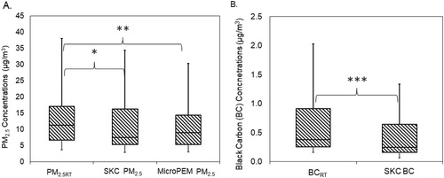
Table 1. PM_2.5 and black carbon (BC) results.

	MicroPEM™ PM2.5	PM2.5RT	SKC PM2.5	SKC BC	BCRT
	(µg/m^3)	(µg/m^3)	(µg/m^3)	(µg/m^3)	(µg/m^3)
Minimum	2.04	3.30	0.32	<LOD	0.09
Maximum	44.20	77.22	54.35	2.18	2.44
Median	8.89	11.21	7.46	0.25	0.38
Mean	12.67	16.28	12.93	0.49	0.68
Winter mean (n = 7–9)	15.42	22.60	16.11	0.31	0.58
Spring mean (n = 5–7)	11.22	10.56	9.51	0.25	0.36
Fall mean (n = 9–12)	7.71	10.06	10.13	0.62	0.79
Summer mean (n = 1–3)	19.79	29.53	23.04	1.38	1.81

LOD for BC = 0.12 µg/m³, <LOD = LOD/√2.

Table 2. Spearman’s coefficients and Wilcoxon p-values of SKC PM_2.5, MicroPEM™ PM_2.5, PM_2.5RT, SKC BC and BC_RT.

	Spearman’s coefficient		Wilcoxon p-value
Method	SKC rs	MicroPEM™ PM2.5 rs	SKC rs	MicroPEM™ PM2.5
PM2.5RT	PM2.5: 0.77***	0.62***	PM2.5: 0.016*	0.002**
MicroPEM™ PM2.5	PM2.5: 0.74***	–	PM2.5: 0.08	–
BCRT	BC: 0.77***	NA	BC: <0.001***	NA

*p < 0.0167, **p < 0.01,***p < 0.001; NA, not analyzed.

The BC medians from the SKC BC and the BC_RT ranged from 0.3 to 0.4 µg/m³, and the means ranged from 0.5 to 0.7 µg/m³ (Table 1 and Figure 2b). There was a significant correlation between the BC_RT and the SKC BC (r = 0.77, p < 0.001) (Table 2). Based on Wilcoxon test, there was a significant difference (p < 0.01, n = 23) between the medians of BC_RT and SKC BC.

The results from blank samples of MicroPEM™ PM_2.5, SKC PM_2.5, and SKC BC averaged at 1.86 µg/m³, 1.25 µg/m³, and 0.03 µg/m³, respectively. The blank values were subtracted from the respective sample values.

3.3. Models and coefficient of variation for PM_2.5

The mean of the CFs developed for the PM_2.5RT using the MicroPEM™ PM_2.5 was 0.94 (CF₁ = MicroPEM™ PM_2.5/PM_2.5RT) with a range of 0.17 - 4.38 and a CV of 84% (Table 3). The multiple regression model, which was selected based on the lowest AIC, included PM_2.5RT values, seasons, hardwood flooring, distance to highway, number of trucks, and open windows during sampling (Equation (3)(3) $$\begin{array}{c}\mathrm{L}\mathrm{N}\left({\text{PM}}_{2.5}\right)=1.125+ \mathrm{L}\mathrm{N}\left(\mathbf{P}{\mathbf{M}}_{\mathbf{2.5}\mathbf{R}\mathbf{T}}\right)*0.5834 +{\beta }_1*0.2269 +{\beta }_2*0.07286 \\ -{\beta }_3*0.1063 –{\beta }_4*0.3587 -{\beta }_5*0.3975–{\mathbf{\beta }}_6*0.0004078 +{\beta }_7*0.00003905\end{array}$$(3) ). The significant variables in the linear regression included the PM_2.5RT and distance to highway (Table 4). Bolded values in Equations (3)–(5) indicate significant parameters. LN is the natural logarithm. When using the multiple regression model to predict the MicroPEM™ PM_2.5 values based on home characteristic variables and PM_2.5RT values, the CV was calculated to be 54% (Table 3). (3) $$\begin{array}{c}\mathrm{L}\mathrm{N}\left({\text{PM}}_{2.5}\right)=1.125+ \mathrm{L}\mathrm{N}\left(\mathbf{P}{\mathbf{M}}_{\mathbf{2.5}\mathbf{R}\mathbf{T}}\right)*0.5834 +{\beta }_1*0.2269 +{\beta }_2*0.07286 \\ -{\beta }_3*0.1063 –{\beta }_4*0.3587 -{\beta }_5*0.3975–{\mathbf{\beta }}_6*0.0004078 +{\beta }_7*0.00003905\end{array}$$(3)

Table 3. Summary statistics for coefficient of variation.

Parameter	Filter	Real-time (RT)	Correction factor (filter/RT)	Coefficient of variation correction Factor	Coefficient of variation linear regression
PM2.5	MicroPEM™ PM2.5 (n = 33)	PM2.5RT	0.94	84%	54% (Equation (3)(3) $$\begin{array}{c}\mathrm{L}\mathrm{N}\left({\text{PM}}_{2.5}\right)=1.125+ \mathrm{L}\mathrm{N}\left(\mathbf{P}{\mathbf{M}}_{\mathbf{2.5}\mathbf{R}\mathbf{T}}\right)*0.5834 +{\beta }_1*0.2269 +{\beta }_2*0.07286 \\ -{\beta }_3*0.1063 –{\beta }_4*0.3587 -{\beta }_5*0.3975–{\mathbf{\beta }}_6*0.0004078 +{\beta }_7*0.00003905\end{array}$$(3) )
PM2.5	SKC PM2.5 (n = 24)	PM2.5RT	0.83	52%	25% (Equation (4)(4) $$\begin{array}{c}\mathrm{L}\mathrm{N}\left({\text{PM}}_{2.5}\right)=-41.49+ \mathrm{L}\mathrm{N}\left(\mathbf{P}{\mathbf{M}}_{\mathbf{2.5}\mathbf{R}\mathbf{T}}\right)*1.428 +{\beta }_1*0.2744 –{\beta }_2*1.700–{\beta }_3*0.08725 +{\mathbf{\beta }}_4*1.902 –{\beta }_8*0.07874 +{\beta }_9*0.7817 +{\beta }_{10}*1.447 -{\beta }_{11}*2.423 –{\beta }_{12}*0.6021 +{\mathbf{\beta }}_{13}*1.149 +{\beta }_{14}*1.472 -{\beta }_6*0.0004267 +{\beta }_{15}*0.0001586 -{\beta }_7*0.00002574 +{\mathbf{\beta }}_{16}*0.01969\end{array}$$(4) )
BC	SKC BC (n = 23)	BCRT	0.74	36%	56% (Equation (5)(5) $$\begin{array}{c}\mathrm{L}\mathrm{N} \left(\mathrm{B}\mathrm{C}\right)=-1.660+ \mathrm{L}\mathrm{N}\left(\mathbf{B}{\mathbf{C}}_{\mathbf{RT}}\right)*0.6920+{\beta }_{12}*0.5493 -{\beta }_{13}*0.5276 +{\beta }_{14}*3.584 -{\beta }_6*0.0003534-{\mathbf{\beta }}_{15}*0.0001418 –{\mathbf{\beta }}_7*0.00007527\end{array}$$(5) )

Table 4. Variables that were included in the multiple regression models with regression estimates (β) and p-values.

	LN MicroPEM™ PM2.5		LN SKC PM2.5		LN SKC BC
	β	p-value	β	p-value	β	p-value
Intercept	1.13	<0.05*	-41.49	<0.05*	–1.66	0.08
LN (PM2.5RT)	0.58	<0.001***	1.43	<0.01**	excl	excl
LN (BCRT)	excl	excl	excl	excl	0.69	<0.01**
Spring	0.23	0.43	0.27	0.72	–	–
Summer	0.07	0.86	–1.70	0.16	–	–
Winter	–0.11	0.70	–0.09	0.82	–	–
Hardwood flooring	–0.36	0.17	1.90	<0.05*	–	–
Cats or dogs present	–	–	0.78	0.11	–	–
Open windows during sampling	–0.40	0.11	–	–	–	–
Kitchen fan during sampling	–	–	–	–	–	–
Frying food during sampling	–	–	1.45	0.05	–	–
Burning candles during sampling	–	–	–2.42	0.08	–	–
Cleaning activities during sampling	–	–	–0.60	0.17	0.55	0.11
HEPA/electrostatic filter in HVAC	–	–	1.15	<0.05*	–0.53	0.30
ECAT score	–	–	1.47	0.51	3.58	0.05
Distance to highway	–0.0004	<0.05*	–0.0004	0.11	–0.0004	0.07
Distance to interstate	–	–	0.0002	0.09	–0.0001	<0.05*
Number of trucks	0.00004	0.10	–0.00003	0.50	–0.00008	<0.05*
People smoking in home	–	–	–0.08	0.92	–	–
Year home built	–	–	0.02	<0.05*	–	–
	R^2 = 0.64		R^2 = 0.94		R^2 = 0.85

**p < 0.01, *p < 0.05;

'–' Not included in model based on the Akaike information criterion;

excl – excluded from regression.

In Equation (3)(3) $$\begin{array}{c}\mathrm{L}\mathrm{N}\left({\text{PM}}_{2.5}\right)=1.125+ \mathrm{L}\mathrm{N}\left(\mathbf{P}{\mathbf{M}}_{\mathbf{2.5}\mathbf{R}\mathbf{T}}\right)*0.5834 +{\beta }_1*0.2269 +{\beta }_2*0.07286 \\ -{\beta }_3*0.1063 –{\beta }_4*0.3587 -{\beta }_5*0.3975–{\mathbf{\beta }}_6*0.0004078 +{\beta }_7*0.00003905\end{array}$$(3) , binary variables are 1 yes and 0 no for: β₁ spring (Apr–Jun), β₂ summer (Jul–Sept), β₃ winter (Jan–Mar), β₄ hardwood flooring, and β₅ opened windows during sampling. Continuous variables are β₆ distance to highway (ranging 26–3157 miles) and β₇ number of trucks < 400 meters (0–20,700).

The mean of the CFs developed for the PM_2.5RT using the SKC PM_2.5 was 0.83 (CF₂ = SKC PM_2.5/PM_2.5RT) with a range of 0.05 – 1.98 and a CV of 52% (Table 3). From the regression predictions of SKC PM_2.5 using PM_2.5RT values, the CV was calculated to be 25% (Equation (4)(4) $$\begin{array}{c}\mathrm{L}\mathrm{N}\left({\text{PM}}_{2.5}\right)=-41.49+ \mathrm{L}\mathrm{N}\left(\mathbf{P}{\mathbf{M}}_{\mathbf{2.5}\mathbf{R}\mathbf{T}}\right)*1.428 +{\beta }_1*0.2744 –{\beta }_2*1.700–{\beta }_3*0.08725 +{\mathbf{\beta }}_4*1.902 –{\beta }_8*0.07874 +{\beta }_9*0.7817 +{\beta }_{10}*1.447 -{\beta }_{11}*2.423 –{\beta }_{12}*0.6021 +{\mathbf{\beta }}_{13}*1.149 +{\beta }_{14}*1.472 -{\beta }_6*0.0004267 +{\beta }_{15}*0.0001586 -{\beta }_7*0.00002574 +{\mathbf{\beta }}_{16}*0.01969\end{array}$$(4) and Table 3). The regression model based on the SKC PM_2.5 included PM_2.5RT values, seasons, type of flooring, cats or dogs present, HEPA or electrostatic filter reported in HVAC, ECAT score, distance to highway, distance to interstate, number of trucks, number of people smoking in home, year the home was built, and activities during sampling such as frying food, burning candles, and cleaning. The significant variables in the SKC PM_2.5 linear regression included the PM_2.5RT, type of flooring, HEPA or electrostatic filter in the HVAC, and the year the home was built (Table 4). (4) $$\begin{array}{c}\mathrm{L}\mathrm{N}\left({\text{PM}}_{2.5}\right)=-41.49+ \mathrm{L}\mathrm{N}\left(\mathbf{P}{\mathbf{M}}_{\mathbf{2.5}\mathbf{R}\mathbf{T}}\right)*1.428 +{\beta }_1*0.2744 –{\beta }_2*1.700–{\beta }_3*0.08725 +{\mathbf{\beta }}_4*1.902 –{\beta }_8*0.07874 +{\beta }_9*0.7817 +{\beta }_{10}*1.447 -{\beta }_{11}*2.423 –{\beta }_{12}*0.6021 +{\mathbf{\beta }}_{13}*1.149 +{\beta }_{14}*1.472 -{\beta }_6*0.0004267 +{\beta }_{15}*0.0001586 -{\beta }_7*0.00002574 +{\mathbf{\beta }}_{16}*0.01969\end{array}$$(4)

In Equation (4)(4) $$\begin{array}{c}\mathrm{L}\mathrm{N}\left({\text{PM}}_{2.5}\right)=-41.49+ \mathrm{L}\mathrm{N}\left(\mathbf{P}{\mathbf{M}}_{\mathbf{2.5}\mathbf{R}\mathbf{T}}\right)*1.428 +{\beta }_1*0.2744 –{\beta }_2*1.700–{\beta }_3*0.08725 +{\mathbf{\beta }}_4*1.902 –{\beta }_8*0.07874 +{\beta }_9*0.7817 +{\beta }_{10}*1.447 -{\beta }_{11}*2.423 –{\beta }_{12}*0.6021 +{\mathbf{\beta }}_{13}*1.149 +{\beta }_{14}*1.472 -{\beta }_6*0.0004267 +{\beta }_{15}*0.0001586 -{\beta }_7*0.00002574 +{\mathbf{\beta }}_{16}*0.01969\end{array}$$(4) , binary variables are 1 yes and 0 no for conditions during sampling including: β₁ spring (Apr–Jun), β₂ summer (Jul–Sept), β₃ winter (Jan–Mar), β₄ hardwood flooring, β₈ smoker or β₉ pets in the home, β₁₀ frying food, β₁₁ burning candles, β₁₂ cleaning, or β₁₃ using a HEPA filter. Continuous variables are β₁₄ ECAT values (ranging 0.29 to 0.88), β₆ distance to highway (ranging 26–3157 miles), β₁₅ distance to interstate (ranging 72–12,687 miles), β₇ number of trucks <400 meters (0–20,700), and β₁₆ the year the home was constructed (ranging 1865 to 2016).

3.4. Model and coefficient of variation for black carbon

The mean CF determined for BC_RT was 0.74 (CF₃ = SKC BC/BC_RT) with a range from 0.04 - 1.13 and a CV of 36% (Table 2). The multiple regression model using the microAeth^® BC_RT yielded a CV of 56% (Equation (5)(5) $$\begin{array}{c}\mathrm{L}\mathrm{N} \left(\mathrm{B}\mathrm{C}\right)=-1.660+ \mathrm{L}\mathrm{N}\left(\mathbf{B}{\mathbf{C}}_{\mathbf{RT}}\right)*0.6920+{\beta }_{12}*0.5493 -{\beta }_{13}*0.5276 +{\beta }_{14}*3.584 -{\beta }_6*0.0003534-{\mathbf{\beta }}_{15}*0.0001418 –{\mathbf{\beta }}_7*0.00007527\end{array}$$(5) and Table 3). The regression model utilized recorded activities during sampling and conditions of the home and included the BC_RT, HEPA or electrostatic filter in the HVAC, ECAT score, distance to highway, distance to interstate, number of trucks, and cleaning during sampling. Significant variables in this model included BC_RT, ECAT score, distance to interstate, and number of trucks (Table 4). (5) $$\begin{array}{c}\mathrm{L}\mathrm{N} \left(\mathrm{B}\mathrm{C}\right)=-1.660+ \mathrm{L}\mathrm{N}\left(\mathbf{B}{\mathbf{C}}_{\mathbf{RT}}\right)*0.6920+{\beta }_{12}*0.5493 -{\beta }_{13}*0.5276 +{\beta }_{14}*3.584 -{\beta }_6*0.0003534-{\mathbf{\beta }}_{15}*0.0001418 –{\mathbf{\beta }}_7*0.00007527\end{array}$$(5)

In Equation (5)(5) $$\begin{array}{c}\mathrm{L}\mathrm{N} \left(\mathrm{B}\mathrm{C}\right)=-1.660+ \mathrm{L}\mathrm{N}\left(\mathbf{B}{\mathbf{C}}_{\mathbf{RT}}\right)*0.6920+{\beta }_{12}*0.5493 -{\beta }_{13}*0.5276 +{\beta }_{14}*3.584 -{\beta }_6*0.0003534-{\mathbf{\beta }}_{15}*0.0001418 –{\mathbf{\beta }}_7*0.00007527\end{array}$$(5) , binary variables are 1 yes and 0 no for conditions during sampling including: β₁₂ cleaning or β₁₃ use of a HEPA filter. Continuous variables are β₁₄ ECAT values (ranging 0.29 to 0.88), β₆ distance to highway (ranging 26–3157 miles), β₁₅ distance to interstate (ranging 72–12,687 miles), and β₇ number of trucks < 400 meters (0–20,700).

3.5. Validation

Simple linear models developed with the real-time values can be seen in Equations (6)–(8). Using the test dataset, the SKC PM_2.5 simple model yielded a RSS value of 108.08 and the multiple regression model yielded a RSS of 38.73. The MicroPEM™ PM_2.5 simple model yielded a RSS value of 8 and the multiple regression model yielded a RSS of 6.5. Finally the SKC BC simple model yielded 1.90 and the multiple regression model yielded a RSS of 2.02 (Table S2 in SI): (6) $$\text{LN}\hspace{0.17em}(\text{MicroPEM}™{ \text{PM}}_{2.5})=0.5002+\hspace{0.17em}\text{LN}\hspace{0.17em}\left({\text{PM}}_{2.5\text{RT}}\right)*0.6803$$(6) (7) $$\text{LN}\hspace{0.17em}\left({\text{SKC} \text{PM}}_{2.5}\right)=-0.3495 + \hspace{0.17em}\text{LN}\hspace{0.17em}\left({\text{PM}}_{2.5\text{RT}}\right)*0.9723$$(7) (8) $$\text{LN}\hspace{0.17em}(\text{SKC} \text{BC})=-0.4214 + \hspace{0.17em}\text{LN}\hspace{0.17em}\left({\text{BC}}_{\text{RT}}\right)*1.1972$$(8)

The measured values SKC PM_2.5, the MicroPEM™ PM_2.5, and SKC BC were compared to the predicted values when the real-time averages were entered into the 3 multiple regression models and the 3 simple models. The predictive multiple regression model values for SKC PM_2.5 (r = 0.83, p < 0.001) and the MicroPEM™ PM_2.5 (r = 0.77, p < 0.001) were more strongly correlated to the measured values than the simple models, respectively (r = 0.77, p < 0.001 and r = 0.62, p < 0.001). The predictive multiple regression and simple model values for SKC BC were equally correlated to the measured values (r = 0.84, p < 0.001) (Table S2 in SI). No significant differences were found between the measured values and the multiple regression models (SKC PM_2.5, p = 0.30; the MicroPEM™ PM_2.5, p = 0.62; and SKC BC, p = 0.48), or between the measured values and the simple models (SKC PM_2.5, p = 0.05; the MicroPEM™ PM_2.5, p = 0.19; and SKC BC, p = 0.04) (Table S2 in SI).

3.6. NIOSH criterion

When evaluating the 95% CI of MicroPEM™ multiple regression model, the error from the reference (MicroPEM™ PM_2.5) ranged –26% to 9%; this model was the closest to obtain the desired criterion of ± 25% (Table S3 in SI ). The 95% CI of the MicroPEM™ simple model had an error percentage of –30% to 4% as compared to the reference. Similarly, the 95% CI of the SKC PM_2.5 multiple regression and simple model compared to the reference ranged from –38% to 36% and –41% to 27%, respectively. Lastly, the SKC BC multiple regression and simple model compared to the reference ranged from –41% to 34% and –45% to 40%, respectively. The real-time data of PM_2.5RT and BC_RT were also compared with MicroPEM™ PM_2.5, SKC PM_2.5 and SKC BC and based on 95% CI, the error percentage ranged from –3% to 88%, –15% to 86%, and –12% to 95%, respectively (Table S3 in SI). Since the method accuracy was worse than 25%, NIOSH recommends that the monitor could only be used for range finding monitoring instead of both compliance and range finding monitoring.

4. Discussion

The concentrations of PM_2.5, as obtained with the PM_2.5RT, the SKC PM_2.5, and the MicroPEM™ PM_2.5 were all significantly correlated with one another. The Wilcoxon test showed no significant differences between the SKC PM_2.5 and the MicroPEM™ PM_2.5. However, the PM_2.5RT was significantly different from both gravimetric filter-analyses (MicroPEM™ PM_2.5 and SKC PM_2.5). The CFs (CF₁ and CF₂) for the PM_2.5RT were 0.94 and 0.83. A CF close to 1 could indicate that minimal correction is needed for accurate PM_2.5RT results. However, both CF1 based on the MicroPEM™ PM_2.5 and CF2 based on the SKC PM_2.5, yielded high CVs (84% and 52%, respectively). Thus, neither CF would provide reproducible results. The multiple regression model took into account variables from the home, such as the season, ECAT score, number of trucks on nearby road, and age of home; this information was obtainable with no extra costs. A more thorough exploration into the properties of the particles detected by the sensors, and how the different environmental conditions may affect the ability of the sensor to accurately convey a signal was not possible. The variables were continuously changing including temperature, humidity, and activities that generated a mixture particles with different sizes and compositions; the variables were also occurring simultaneously and were not controlled for or continuously monitored by the sampling team. By utilizing the multiple regression models, the CV was calculated to be 54% using the MicroPEM™ PM_2.5, and 25% using SKC PM_2.5. Both regression models would yield more reliable results than CF₁ and CF₂, respectively. The validation demonstrated that the multiple regression models for SKC PM_2.5 and MicroPEM™ PM_2.5 were a tighter fit to the data compared to the simple regression models, as their RSS values were lower. The multiple regression models as compared to the filter data yielded higher Spearman’s correlation coefficients as compared to the simple models; however, all correlations were significant. None of the simple or multiple regression models were significantly different than the reference filter data. The MicroPEM™ PM_2.5 multiple regression model was close to achieving the NIOSH criterion that the model’s 95% CI be within 25% of the filter-based data. All other PM_2.5 models and the PM_2.5RT data did not meet this criterion. If a quick exposure estimate is desired when filter analysis is not possible, the real-time data with additional variables in a regression model could provide an approximate exposure estimate. While this estimate will not provide the specific dose exposure data to inform on the health effects relationship, it will provide an approximate assessment to inform control needs.

Overall, the microAeth^® averaged BC_RT concentrations were correlated strongly and significantly with the SKC BC concentrations; however, the paired samples were found to be significantly different. The BC concentrations are comparable to the results of other studies that evaluated indoor BC concentrations associated with TRAP. LaRosa et al. (2002) measured BC every 5 min for two years inside suburban home outside of Washington, D.C. They found a mean indoor BC concentration of 0.5 µg/m³, which was the same as our mean obtained from the SKC BC. The BC correction factor (CF₃) utilizing the SKC BC yielded a CV of 36%. When the multiple regression model was applied, the added information did not improve the CV. None of the variables added into the regression appeared to help predict the indoor BC levels. In addition, the validation demonstrated that the simple model for SKC BC was a tighter fit to the data compared to the multiple regression model, as the RSS value was lower. The multiple regression model as compared to the filter data yielded higher Spearman’s correlation coefficient as compared to the simple model; however, both correlations were significant. Neither the multiple regression or simple model was significantly different than the reference filter data, nor did they meet the NIOSH criterion that the model’s 95% CI be within 25% of the filter-based data. Perhaps a more detailed evaluation of the variables such as duration during cooking or burning candles would provide a more detailed regression analysis and generate a lower CV. Seasonal influences, home characteristics, and activities can contribute to the BC concentrations within the home (Dons et al. 2011).

The PM_2.5 concentrations were similar to those found in other studies of indoor air pollution. Tunno et al. (2015) evaluated industry-impacted homes and reported indoor mean concentrations for PM_2.5 to be 18.9 µg/m³ from January to March (winter). Our average PM_2.5 concentrations from winter were consistent with Tunno et al. with values of 15.4 µg/m³ from MicroPEM™ PM_2.5, 22.6 µg/m³ from PM_2.5RT, and 16.1 µg/m³ from SKC PM_2.5. In the study by Fischer et al. (2000), the average PM_2.5 concentration in homes close to high traffic was determined to be 27 µg/m³ and in homes close to low traffic was determined to be 12 µg/m³. In this case, our findings were more consistent with the homes close to low traffic with PM_2.5 means of 12.7 µg/m³ from MicroPEM™ PM_2.5, 16.3 µg/m³ PM_2.5RT, and 12.9 µg/m³ from SKC PM_2.5. The definition of traffic exposure was different between the study by Fisher et al. and the current study. We used a land-use regression calculation for the estimation of elemental carbon whereas Fischer et al. determined traffic intensity based on if the street was considered a main street or a side street. When investigating various traffic-related pollutants, Kingham et al. (2000) determined a mean of 17.8 µg/m³ for PM_2.5 concentrations. Our average PM_2.5 concentrations were slightly lower but similar. Alternatively, Landis et al. (2001) explored general exposure to PM_2.5 that was not specifically associated with TRAP, and found a mean PM_2.5 concentration of 6.7 µg/m³. This is much lower than our PM_2.5 means of homes that were considered to be impacted by TRAP.

While both multiple regression linear regression models for PM_2.5 were similar, the best subsets of independent variables and the best models were selected based on the lowest AIC; therefore, the variables selected and the estimated coefficients were different between the two models. The following variables were selected for one, but not both of the PM_2.5 models: presence of cats or dogs, HEPA or electrostatic filter reported in HVAC, ECAT score, distance to interstate, the year the home was built, number of people smoking in home, and activities during sampling such as frying food, burning candles, opening windows, and cleaning. Frying food was selected into the regression model utilizing the SKC PM_2.5, but not for the MicroPEM PM_2.5 regression model. Cooking is a primary source of PM with frying food being among the top three methods with the highest mass emission rates (Torkmahalleh et al. 2012; Tunno et al. 2015). Perhaps if more detailed information was obtained regarding the cooking, such as duration and frequency, this variable could have been included in the best subsets of independent variables into both regression models. Both models for PM_2.5-included seasonal variations, flooring type, distance to highway, and number of trucks. Factors contributing to TRAP, such as distance to highway and trucks on roadways are a contributing source of PM_2.5 in TRAP (Charron and Harrison 2005). Similar to the current study, seasonality differences in PM_2.5 have been seen in other studies; Tunno et al. (2015) and Clements et al. (2018) found a mean indoor PM_2.5 was higher, on average, during summer (25 µg/m³ and 10.6 µg/m³, respectively) than winter (19 µg/m³ and 6.1 µg/m³, respectively). In the current study, the average SKC PM_2.5 was 23 µg/m³ in the summer and 16 µg/m³ in the winter. The age of the building (year of construction) has been shown to be among the most influential factors related to air leakage (Chan et al. 2003). Newer homes are typically “tighter” and have lower air infiltration and leakage as compared to older homes (Sherman and Chan 2004; Stephens and Siegel 2012b). The slightly positive correlation with the year home was built implied the PM_2.5 sources could be from indoors, and that these particles have less of a chance to “leak” into the outdoor environment in newer homes. As the buildings became newer and “tighter,” the PM_2.5 increased. The type of flooring can affect the volume and particle size of resuspension. The velocity and turbulence of the activity on that flooring affects the particle size that is disturbed (Mukai, Siegel and Novoselac 2009), which could impact the resuspension of PM_2.5. Tian et al. (2014) demonstrated that higher humidity can enhance resuspension on high-density cut pile carpet, and the opposite effect was observed on hard floorings. In addition to potentially more informative variables, such as the duration and frequency of activities, another limitation of the study was the number of samples. A larger sample size could possibly produce more similar models with respect to variables and coefficient estimates.

Technology is rapidly changing making it easier, quicker and less expensive to conduct exposure assessment for individuals. Instruments such as real-time sensors are the future of air quality assessment; however, they can have reduced accuracy and precision. Therefore, to take advantage of these instruments, we need to ensure that the instruments meet designated criterion or correlation with a more accurate method. The linear regression models provided here for PM_2.5 provide alternative strategies to reduce the need for filter analyses, saving time and resources so that larger-scale studies can be performed. In addition, these instruments have the potential to easily and quickly inform the user the best approach to control the exposure unlike filter-based methods. Improving the instrument’s accuracy so that it correlates strongly with filter-based methods will allow for consistency in exposure evaluations, larger-scale data to be collected and subsequent improved air quality.

5. Conclusion

This study addressed the need for accurate, cost-effective methods for rapid assessment of TRAP. The objective of this study was to create a CF and linear regression model for the real-time measurements of the RTI’s Micro Personal Exposure Monitor (MicroPEM™) and microAeth^® black carbon (AE51) sensor to generate accurate real-time data for PM_2.5 (PM_2.5RT) and black carbon (BC_RT) in Cincinnati metropolitan homes. By improving the accuracy of these compact, personal exposure, real-time sensors, the need for cumbersome, expensive filter analysis will be unnecessary. The BC multiple regression model yielded no improvement of BC_RT as compared to the SKC BC. The PM_2.5 multiple regression models reduced the variation of PM_2.5RT as compared to SKC PM_2.5; however, it was not clear which model yielded the best accuracy until analyzed using the NIOSH criterion. Only the multiple regression model developed for the MicroPEM™ PM_2.5 was borderline to the criterion. The results from this study will help to improve the accuracy of PM_2.5 monitoring after an appropriate statistical model is applied. The advantage of this approach is that it eliminates the need for costly filter-based analyses which could allow for accurate large-scale health-focused studies.

Disclosure statement

No potential conflict of interest was reported by the authors.

Additional information

Funding

This work was supported by U.S. Department of Housing and Urban Development (Grant OHHHU0027-14). Jennie Cox was supported by the National Institute for Occupational Safety and Health through the University of Cincinnati Education and Research Center (No. T42OH008432).

References

- Andreae, M., and A. Gelencsér. 2006. Black carbon or brown carbon? The nature of light-absorbing carbonaceous aerosols. Atmos. Chem. Phys. 6 (10):3131–3148. doi:10.5194/acp-6-3131-2006.
- Apte, J. S., T. W. Kirchstetter, A. H. Reich, S. J. Deshpande, G. Kaushik, A. Chel, J. D. Marshall, and W. W. Nazaroff. 2011. Concentrations of fine, ultrafine, and black carbon particles in auto-rickshaws in New Delhi, India. Atmos. Environ. 45 (26):4470–4480. doi:10.1016/j.atmosenv.2011.05.028.
- Ballach, J., R. Hitzenberger, E. Schultz, and W. Jaeschke. 2001. Development of an improved optical transmission technique for black carbon (BC) analysis. Atmos. Environ. 35 (12):2089–2100. doi:10.1016/S1352-2310(00)00499-4.
- Bernstein, J. A., N. Alexis, H. Bacchus, I. L. Bernstein, P. Fritz, E. Horner, N. Li, S. Mason, A. Nel, J. Oullette, K. Reijula, T. Reponen, J. Seltzer, A. Smith, and S. M. Tarlo. 2008. The health effects of nonindustrial indoor air pollution. J. Allergy Clinical Immunol. 121 (3):585–591. doi:10.1016/j.jaci.2007.10.045.
- Billings, P. G., J. E. Nolan, L. Alexander, L. K. Bender, D. V. Vleet, Z. Jump, S. Rappaport, J. M. Samet, N. Ballentine, T. Nimirowski., et al. 2018. State of the air 2018. Chicago, IL: American Lung Association.
- Chan, W. R., P. N. Price, M. D. Sohn, and A. J. Gadgil. 2003. Analysis of US residential air leakage database. Berkeley, CA: Lawrence Berkeley National Laboratory.
- Charron, A., and R. M. Harrison. 2005. Fine (PM2. 5) and coarse (PM2. 5-10) particulate matter on a heavily trafficked London highway: sources and processes. Environ. Sci. Technol. 39:7768–7776. doi:10.1021/es050462i.
- Cho, S.-H., R. T. Chartier, K. Mortimer, M. Dherani, and T. Tafatatha. 2016. A personal particulate matter exposure monitor to support household air pollution exposure and health studies. In Global Humanitarian Technology Conference (GHTC), 2016, IEEE, 817–818.
- Clark, M. L., S. J. Reynolds, J. B. Burch, S. Conway, A. M. Bachand, and J. L. Peel. 2010. Indoor air pollution, Cookstove quality, and housing characteristics in two Honduran communities. Environ. Res. 110 (1):12–18. doi:10.1016/j.envres.2009.10.008.
- Clements, N., P. Keady, J. B. Emerson, N. Fierer, and S. L. Miller. 2018. Seasonal variability of airborne particulate matter and bacterial concentrations in Colorado homes. Atmosphere 9 (4):133. doi:10.3390/atmos9040133.
- Cox, J., K. Isiugo, P. Ryan, S. A. Grinshpun, M. Yermakov, C. Desmond, R. Jandarov, S. Vesper, J. Ross, S. Chillrud, K. Dannemiller, and T. Reponen. 2018. Effectiveness of a portable air cleaner in removing aerosol particles in homes close to highways. Indoor Air 28 (6):818–827. doi:10.1111/ina.12502.
- Dons, E., L. I. Panis, M. Van Poppel, J. Theunis, H. Willems, R. Torfs, and G. Wets. 2011. Impact of time–activity patterns on personal exposure to black carbon. Atmos. Environ. 45 (21):3594–3602. doi:10.1016/j.atmosenv.2011.03.064.
- Dutmer, C. M., A. M. Schiltz, A. Faino, N. Rabinovitch, S.-H. Cho, R. T. Chartier, C. E. Rodes, J. W. Thornburg, and A. H. Liu. 2015. Accurate assessment of personal air pollutant exposures in inner-city asthmatic children. J. Allergy Clin. Immunol. 135 (2):AB165. doi:10.1016/j.jaci.2014.12.1478.
- Ferro, A. R., R. J. Kopperud, and L. M. Hildemann. 2004. Elevated personal exposure to particulate matter from human activities in a residence. J. Expo. Sci. Environ. Epidemiol. 14 (S1):S34. doi:10.1038/sj.jea.7500356.
- Fischer, P. H., G. Hoek, H. van Reeuwijk, D. J. Briggs, E. Lebret, J. H. van Wijnen, S. Kingham, and P. E. Elliott. 2000. Traffic-related differences in outdoor and indoor concentrations of particles and volatile organic compounds in Amsterdam. Atmos. Environ. 34 (22):3713–3722. doi:10.1016/S1352-2310(00)00067-4.
- Gehring, U., A. H. Wijga, M. Brauer, P. H. Fischer, J. C. de Jongste, M. Kerkhof, M. Oldenwening, H. A. Smit, and B. Brunekreef. 2010. Traffic-related air pollution and the development of asthma and allergies during the first 8 years of life. Amer. J. Respiratory Critical Care Med. 181 (6):596–603. doi:10.1164/rccm.200906-0858OC.
- Good, N., A. Mölter, J. L. Peel, and J. Volckens. 2017. An accurate filter loading correction is essential for assessing personal exposure to black carbon using an aethalometer. J. Exposure Sci. Environ. Epidemiol. 27 (4):409. doi:10.1038/jes.2016.71.
- Grahame, T. J., R. Klemm, and R. B. Schlesinger. 2014. Public health and components of particulate matter: the changing assessment of black carbon. J. Air Waste Manage. Assoc. 64 :620–660. doi:10.1080/10962247.2014.912692.
- Hagler, G. S. W., T. L. B. Yelverton, R. Vedantham, A. D. A. Hansen, and J. R. Turner. 2011. Post-processing method to reduce noise while preserving high time resolution in aethalometer real-time black carbon data. Aerosol Air Quality Res. 11 (5):539–546. doi:10.4209/aaqr.2011.05.0055.
- Hansen, A. D. A. 2005. The Aethalometer, 1–209. Berkeley, California, USA: Magee Scientific Company.
- Health Effects Institute 2010. Traffic-related air pollution: a critical review of the literature on emissions, exposure, and health effects. In Health effects institute panel on the health effects of Traffic-Related Air Pollution. Boston, MA: Health Effects Institute.
- Ihaka, R., and R. Gentleman. 1996. R: a language for data analysis and graphics. J. Comput. Graphical Statist. 5:299–314. doi:10.2307/1390807.
- Jamriska, M., L. Morawska, and K. Mergersen. 2008. The effect of temperature and humidity on size segregated traffic exhaust particle emissions. Atmos. Environ. 42 (10):2369–2382. doi:10.1016/j.atmosenv.2007.12.038.
- Jeong, C.-H., A. Traub, and G. J. Evans. 2017. Exposure to ultrafine particles and black carbon in diesel-powered commuter trains. Atmos. Environ. 155:46–52. doi:10.1016/j.atmosenv.2017.02.015.
- Jerrett, M., M. Arain, P. Kanaroglou, B. Beckerman, D. Crouse, N. Gilbert, J. Brook, N. Finkelstein, and M. Finkelstein. 2007. Modeling the intraurban variability of ambient traffic pollution in Toronto, Canada. J. Toxicology Environ. Health, Part A 70 (3–4):200–212. doi:10.1080/15287390600883018.
- Jung, K. H., S. Lovinsky-Desir, B. Yan, D. Torrone, J. Lawrence, J. R. Jezioro, M. Perzanowski, F. P. Perera, S. N. Chillrud, and R. L. Miller. 2017. Effect of personal exposure to black carbon on changes in allergic asthma gene methylation measured 5 days later in urban children: importance of allergic sensitization. Clinical Epigenetics 9 (61):1–11.
- Jung, K. H., M. M. Patel, K. Moors, P. L. Kinney, S. N. Chillrud, R. Whyatt, L. Hoepner, R. Garfinkel, B. Yan, and J. Ross. 2010. Effects of heating season on residential indoor and outdoor polycyclic aromatic hydrocarbons, black carbon, and particulate matter in an urban birth cohort. Atmos. Environ. 44 (36):4545–4552. doi:10.1016/j.atmosenv.2010.08.024.
- Kingham, S., D. Briggs, P. Elliott, P. Fischer, and E. Lebret. 2000. Spatial variations in the concentrations of traffic-related pollutants in indoor and outdoor air in Huddersfield, England. Atmos. Environ. 34 :905–916.
- Kirchstetter, T. W., and T. Novakov. 2007. Controlled generation of black carbon particles from a diffusion flame and applications in evaluating black carbon measurement methods. Atmos. Environ. 41 (9):1874–1888. doi:10.1016/j.atmosenv.2006.10.067.
- Klepeis, N. E., W. C. Nelson, W. R. Ott, J. P. Robinson, A. M. Tsang, P. Switzer, J. V. Behar, S. C. Hern, and W. H. Engelmann. 2001. The national human activity pattern survey (NHAPS): a resource for assessing exposure to environmental pollutants. J. Expo. Sci. Environ. Epidemiol. 11 (3):231–252. doi:10.1038/sj.jea.7500165.
- Landis, M. S., G. A. Norris, R. W. Williams, and J. P. Weinstein. 2001. Personal exposures to PM2.5 mass and trace elements in baltimore, MD, USA. Atmos. Environ. 35 (36):6511–6524. doi:10.1016/S1352-2310(01)00407-1.
- LaRosa, L. E., T. J. Buckley, and L. A. Wallace. 2002. Real-time indoor and outdoor measurements of black carbon in an occupied house: an examination of sources. J. Air Waste Manage. Assoc. 52:41–49. doi:10.1080/10473289.2002.10470758.
- LeMasters, G. K., K. Wilson, L. Levin, J. Biagini, P. Ryan, J. E. Lockey, S. Stanforth, S. Maier, J. Yang, J. Burkle, M. Villareal, G. K. Khurana Hershey, and D. I. Bernstein. 2006. High prevalence of aeroallergen sensitization among infants of atopic parents. J. Pediatrics 149 (4):505–511. doi:10.1016/j.jpeds.2006.06.035.
- Lin, C., N. Masey, H. Wu, M. Jackson, D. J. Carruthers, S. Reis, R. M. Doherty, I. J. Beverland, and M. R. Heal. 2017. Practical field calibration of portable monitors for mobile measurements of multiple air pollutants. Atmosphere 8 (12):231. doi:10.3390/atmos8120231.
- Martuzevicius, D., S. Grinshpun, T. Lee, S. Hu, P. Biswas, T. Reponen, and G. LeMasters. 2008. Traffic-related PM 2.5 aerosol in residential houses located near major highways: indoor versus outdoor concentrations. Atmos. Environ 42 (27):6575–6585. doi:10.1016/j.atmosenv.2008.05.009.
- Minet, L., J. Stokes, J. Scott, J. Xu, S. Weichenthal, and M. Hatzopoulou. 2018. Should traffic-related air pollution and noise be considered when designing urban bicycle networks? Transportation res. Part D: Transport Environment 65:736–749. doi:10.1016/j.trd.2018.10.012.
- Mukai, C., J. Siegel, and A. Novoselac. 2009. Impact of airflow characteristics on particle resuspension from indoor surfaces. Aerosol Sci. Technol. 43 (10):1022–1032. doi:10.1080/02786820903131073.
- National Research Council 2004. Research priorities for airborne particulate matter: Continuing research progress. IV. Washington, DC: National Academies Press.
- NIOSH 2012. Components for evaluation of Direct-Reading monitors for gases and vapors. Cincinnati, OH: National Institute for Occupational Safety and Health.
- Ryan, P., D. Bernstein, J. Lockey, T. Reponen, L. Levin, S. Grinshpun, M. Villareal, G. Khurana Hershey, J. Burkle, and G. LeMasters. 2009. Exposure to traffic-related particles and endotoxin during infancy is associated with wheezing at age 3 years. Amer. J. Respiratory Critical Care Med. 180 (11):1068–1075. doi:10.1164/rccm.200808-1307OC.
- Ryan, P., G. LeMasters, L. Levin, J. Burkle, P. Biswas, S. Hu, S. Grinshpun, and T. Reponen. 2008. A land-use regression model for estimating microenvironmental diesel exposure given multiple addresses from birth through childhood. Sci. Total Environ. 404 (1):139–147. doi:10.1016/j.scitotenv.2008.05.051.
- Sherman, M., and R. Chan. 2004. Building airtightness: research and practice state of the art review, Technical Report No. LBNL-53356, Lawrence Berkeley National Laboratory.
- Sloan, C. D., T. J. Philipp, R. K. Bradshaw, S. Chronister, W. B. Barber, and J. D. Johnston. 2016. Applications of GPS-tracked personal and fixed-location PM2.5 continuous exposure monitoring. J. Air Waste Manage. Assoc. 66:53–65. doi:10.1080/10962247.2015.1108942.
- Stephens, B., and J. Siegel. 2012. Comparison of test methods for determining the particle removal efficiency of filters in residential and light-commercial Central HVAC systems. Aerosol sci. technol. 46 (5):504–513. doi:10.1080/02786826.2011.642825.
- Stephens, B., and J. Siegel. 2012. Penetration of ambient submicron particles into single‐family residences and associations with building characteristics. Indoor Air 22 (6):501–513. doi:10.1111/j.1600-0668.2012.00779.x.
- The National Academies of Sciences Engineering and Medicine 2016. Health risks of indoor exposure to particulate matter: Workshop Summary. Washington, DC: The National Academies of Press.
- Thurston, G., K. Ito, and R. Lall. 2011. A source apportionment of US fine particulate matter air pollution. Atmos. Environ. 45 (24):3924–3936. doi:10.1016/j.atmosenv.2011.04.070.
- Tian, Y., K. Sul, J. Qian, S. Mondal, and A. R. Ferro. 2014. A comparative study of walking‐induced dust resuspension using a consistent test mechanism. Indoor Air 24 (6):592–603. doi:10.1111/ina.12107.
- Torkmahalleh, M., I. Goldasteh, Y. Zhao, N. Udochu, A. Rossner, P. Hopke, and A. Ferro. 2012. PM2.5 and ultrafine particles emitted during heating of commercial cooking oils. Indoor Air 22 (6):483–491. doi:10.1111/j.1600-0668.2012.00783.x.
- Tunno, B., K. Shields, L. Cambal, S. Tripathy, F. Holguin, P. Lioy, and J. Clougherty. 2015. Indoor air sampling for fine particulate matter and black carbon in industrial communities in Pittsburgh. Sci. Total Environ. 536:108–115.
- Vesper, S., R. Prill, L. Wymer, L. Adkins, R. Williams, and F. Fulk. 2015. Mold contamination in schools with either high or low prevalence of asthma. Pediatr Allergy Immunol 26 (1):49–53. doi:10.1111/pai.12324.
- Volpino, P., F. Tomei, C. La Valle, E. Tomao, M. Rosati, M. Ciarrocca, S. De Sio, B. Cangemi, R. Vigliarolo, and F. Fedele. 2004. Respiratory and cardiovascular function at rest and during exercise testing in a healthy working population: effects of outdoor traffic air pollution. Occupational Med. 54 (7):475–482. doi:10.1093/occmed/kqh102.
- Wang, F. 2001. Confidence interval for the mean of non‐normal data. Quality Rel. Eng. Int. 17 (4):257–267. doi:10.1002/qre.400.
- Yan, B., D. Kennedy, R. Miller, J. Cowin, K.-H. Jung, M. Perzanowski, M. Balletta, F. Perera, P. Kinney, and S. Chillrud. 2011. Validating a nondestructive optical method for apportioning colored particulate matter into black carbon and additional components. Atmos. Environ. 45 (39):7478–7486. doi:10.1016/j.atmosenv.2011.01.044.
- Zhang, T., S. Chillrud, J. Ji, Y. Chen, M. Pitiranggon, W. Li, Z. Liu, and B. Yan. 2017. Comparison of PM2.5 exposure in hazy and non-hazy days in Nanjing, China. Aerosol Air Qual Res. 17 (9):2235–2246. doi:10.4209/aaqr.2016.07.0301.