The second ACTRIS inter-comparison (2016) for Aerosol Chemical Speciation Monitors (ACSM): Calibration protocols and instrument performance evaluations

Abstract

This work describes results obtained from the 2016 Aerosol Chemical Speciation Monitor (ACSM) intercomparison exercise performed at the Aerosol Chemical Monitor Calibration Center (ACMCC, France). Fifteen quadrupole ACSMs (Q_ACSM) from the European Research Infrastructure for the observation of Aerosols, Clouds and Trace gases (ACTRIS) network were calibrated using a new procedure that acquires calibration data under the same operating conditions as those used during sampling and hence gets information representative of instrument performance. The new calibration procedure notably resulted in a decrease in the spread of the measured sulfate mass concentrations, improving the reproducibility of inorganic species measurements between ACSMs as well as the consistency with co-located independent instruments. Tested calibration procedures also allowed for the investigation of artifacts in individual instruments, such as the overestimation of m/z 44 from organic aerosol. This effect was quantified by the m/z (mass-to-charge) 44 to nitrate ratio measured during ammonium nitrate calibrations, with values ranging from 0.03 to 0.26, showing that it can be significant for some instruments. The fragmentation table correction previously proposed to account for this artifact was applied to the measurements acquired during this study. For some instruments (those with high artifacts), this fragmentation table adjustment led to an “overcorrection” of the f44 (m/z 44/Org) signal. This correction based on measurements made with pure NH₄NO₃, assumes that the magnitude of the artifact is independent of chemical composition. Using data acquired at different NH₄NO₃ mixing ratios (from solutions of NH₄NO₃ and (NH₄)₂SO₄) we observe that the magnitude of the artifact varies as a function of composition. Here we applied an updated correction, dependent on the ambient NO₃ mass fraction, which resulted in an improved agreement in organic signal among instruments. This work illustrates the benefits of integrating new calibration procedures and artifact corrections, but also highlights the benefits of these intercomparison exercises to continue to improve our knowledge of how these instruments operate, and assist us in interpreting atmospheric chemistry.

EDITOR:

• Jim Smith

Introduction

Continuous and long-term measurements of essential climatologically relevant parameters, such as aerosol chemistry and physical properties, are critical to resolve aerosol-cloud-climate interactions and to gain insights into the role they play in climate change and air quality. Recently in Europe, significant efforts have contributed to the installation and maintenance of a number of different observation stations in a range of differing environments (Fröhlich et al. 2015a; Hari and Kulmala 2005; O’Connor, Jennings, and O’Dowd 2008; Petit et al. 2015; Ripoll et al. 2015). These stations notably belong to the European Research Infrastructure for the observation of Aerosol, Clouds, and Trace Gases (ACTRIS, www.actris.eu).

The physical and chemical properties of aerosols are measured at a number of stations. Up until recently, aerosol chemistry was acquired through offline filter measurements, or over short periods using more advanced techniques such as aerosol mass spectrometry (Canagaratna et al. 2007). Development of the Aerosol Chemical Speciation Monitor (ACSM) allows near-autonomous continuous measurements of aerosol chemistry, with minimal intervention from the user. The ACSM uses either a quadrupole mass spectrometer (Q-ACSM) (Ng et al. 2011) or a time of flight mass spectrometer (ToF-ACSM) (Fröhlich et al. 2013) to measure particle composition. This instrument designed specifically for in-situ measurements of non-refractory submicron (NR-PM₁) aerosol species has a time resolution of approximately 15 to 30 min. It is based on aerosol mass spectrometry (AMS) technology and has demonstrated its suitability for continuous monitoring over the last eight years. More recent advances in this instrument include a newly designed aerosol inlet and capture vaporizer capable of sampling aerosol particles having diameters up to 2.5 microns (Xu et al. 2017; Zhang et al. 2017). Aerosol chemistry measurements are being increasingly used to constrain predictive models to forecast atmospheric processes and evolution (e.g., Ciarelli et al. 2017; Bessagnet et al. 2016), and therefore it is imperative to ensure high quality data to develop and evaluate these models. To satisfy this need, a number of calibration centers have been created in Europe with the specific objective to identify measurement guidelines and calibration procedures. The Aerosol Chemical Monitor Calibration Center (ACMCC) is part of the European Center for Aerosol Calibration (ECAC, www.actris-ecac.eu), and is oriented towards the calibration of online aerosol chemistry measurements (Crenn et al. 2015). It notably aims to calibrate and intercompare ACSM instruments used at ACTRIS stations at least every three years, so to ensure the continuity of long-term quality assured data within this research infrastructure. The first ACSM intercomparison took place at the ACMCC in December 2013. During this first exercise, a detailed statistical analysis was performed on instrument sensitivities and the inter-comparability of the different variables measured by the ACSM instruments (Crenn et al. 2015b). In addition, the source apportionment of the organic aerosol measured from these instruments was compared over a three week period (Fröhlich et al. 2015b). The result of the 2013 inter-comparison exercise illustrated good agreement between these instruments, but highlighted variability in the sulfate and organic aerosol species. This manuscript describes results from a second intercomparison exercise, held in March 2016, at the ACMCC. This intercomparison specifically addressed new recommended calibration procedures, and evaluated recently proposed corrections for artifacts related to the organic aerosol measurements.

Methodology

Description of the site and experimental set up

A total of 15 Q-ACSM instruments were installed at the Site Instrumental de Recherche par Télédétection Atmosphérique (SIRTA) station during the month of March 2016. The SIRTA station is an ACTRIS national facility for aerosol, cloud, and gas-phase measurements and is located 20 km south of Paris, in Gif-sur-Yvette. Similar to the set up used during the first ACSM inter-laboratory intercomparison (ILC) in 2013 (Crenn et al. 2015), instruments were organized into three groups of four instruments, and one group of three instruments. Four separate PM_2.5 inlets were used to deliver ambient aerosols into the laboratory. Behind each inlet were four instruments, each one of these instruments had an individual nafion dryer with integrated relative humidity (RH) measurements in the aerosol sampling line. The temperature difference between the outside and the inside of the laboratory, together with the nafion dryers meant that the aerosol sample flow RH did not exceed 40%. All instruments were operating with a time resolution of approximately 30 min. Particle-free air sampling was performed prior to and after the intercomparison campaign, ensuring that no leaks or contamination were occurring inside the station or in the sampling lines. These measurements were performed by placing a total particle filter in place of the PM₁ inlet for approximately two hours, providing a total of four points per filter period.

Q–ACSM

Briefly, the Q-ACSM instrument is based on the same technology as the aerosol mass spectrometer (AMS), using an aerodynamic lens with greater than 50% transmission efficiency of particle sizes (D_p) between 75 nm and 650 nm, a vaporizer at 600 °C, and electron impact ionization at 70 eV (Liu et al. 2017). In the ACSM instrument, the principal difference compared to the AMS is the lack of size resolved data. For the extraction of different chemical species from the mass spectral data, the ACSM uses the same fragmentation table as the AMS (Allan et al. 2004). Data analysis was performed using the Igor Pro (Wavemetrics, v6.3.7) procedure acsm_local (v1.5.11.1).

Co-located measurements

A number of instruments were operated alongside the Q-ACSM instruments at the SIRTA site. These instruments included the Fine Dust Aerosol Spectrometer (FIDAS^®, PALAS), providing size-segregated particle mass concentrations every 15 min over a total of 64 size bins ranging from 180 nm up to 18,000 nm. A tapering element oscillating microbalance equipped with filter dynamic measurement system (TEOM-FDMS, Ecomesure) provided total particle mass concentration of the PM₁ component. Aerosol particle composition was measured using an online particle into liquid sampler (PILS) coupled with online ion chromatography (IC, Dionex), providing information on the concentrations of water-soluble anion species (including NO₃⁻ and SO₄²⁻) of both refractory and non-refractory particles with a temporal resolution of approximately 5 min. Mass concentration of NH₄⁺ was not measured by the PILS-IC but is calculated based on the anionic concentrations of NO₃⁻, Cl⁻, and SO₄²⁻, assuming that all these species exist as NH₄NO₃, NH₄Cl, and (NH₄)₂SO₄. Based on the inlet set up and flow rate, the cut off diameter of the PILS-IC instrument was calculated to be approximately 1.4 µm. A Sunset Laboratory Organic Carbon Elemental Carbon (OC/EC) field analyzer measured the PM₁ organic and elemental carbon content of aerosol particles (OC/EC) with a resolution of approximately 2 h. A denuder was placed upstream of the instrument to remove gas-phase species. The analysis of the OC/EC followed the European standards recommendation using the EUSAAR2 thermal protocol (Cavalli et al. 2010). Based on previous studies at the site, it was assumed that the contribution of secondary organic aerosol was dominant and hence the OM to OC ratio applied to the sunset OC measurements was 2.1 (Sciare et al. 2011). A comparison between the PM₁ PILS + OM measurements with that of PM₁ TEOM measurements illustrated that despite the differences in the calculated inlet size cutoff there was good agreement between the two sets of measurements (Figure S1).

RIE calibration principles and set up

A new calibration method specifically aimed at improving the ACSM relative ionization efficiency (RIE) of NH₄ and SO₄ was introduced during this intercomparison exercise. Until now, the SO₄ RIE was determined using the jump scan (JS) mode in the ACSM software. In JS mode, only specific m/z values are measured, instead of scanning the full range (10 to 150 amu) of the mass spectrometer. For NH₄NO₃ (AN), the measured m/z’s are 15 (NH⁺), 16 (NH₂⁺), 17 (NH₃⁺), 30 (NO⁺), and 46 (NO₂⁺), and for (NH₄)₂SO₄ (AS) the m/z’s are 15 (NH⁺), 16 (NH₂⁺), 17 (NH₃⁺), 48 (SO⁺), 64 (SO₂⁺), 80 (SO₃⁺), 81 (HSO₃⁺), and 98 (H₂SO₄⁺). The advantage of JS compared to the regular acquisition mode is that it takes less time to acquire the mass spectral information; however, for some species such as SO₄, particles can take longer to completely vaporize and the fast timing of JS mode can lead to erroneously low RIE values. In the new recommended calibration procedure, size-selected particles of either AN and/or AS are measured in full scan (FS) acquisition mode, where the entire mass spectrum is scanned as would be done during ambient sampling but the same ions as those measured in JS are used in the analysis. Since the full mass spectral range is scanned, this approach has the added advantage of identifying any m/z artifacts that exist in the instrument. In both the JS and FS modes, NH₄ RIE is determined from the ratio of the slopes of signal versus input mass plots of NH₄ and NO₃ measured from pure NH₄NO₃. The SO₄ RIE is then determined from the product of the NH₄ RIE and the ratio of the slopes of signal versus input mass plots of SO₄ and NH₄ from pure (NH₄)₂SO₄ (Budisulistiorini et al. 2014). The response factor of NO₃, which is proportional to the ionization efficiency, was determined using both the JS and FS. Since NH₄NO₃ can rapidly vaporize, the response factor remains similar in both calibration modes. However, the FS mode is recommended for consistency with operating conditions during ambient sampling.

For all calibrations, aqueous solutions of ammonium nitrate (AN) and/or ammonium sulfate (AS) were used. These solutions were atomized into the instrument as either pure AN and pure AS solutions or as solutions containing mass ratios of 2:1 (AN:AS) and 1:2 (AN:AS) mixtures. The purpose of using these mixed solutions was to evaluate how the mass fraction of a certain species might influence its calibration value, and secondly it provided a means to compare the NH₄ RIE determined from pure AN particles with that obtained from the combined pure and mixed AN/AS data. The atomized solutions then passed through two silica gel dryers, and into a Differential Mobility Analyzer (DMA, TSI 3800) which selected particles with electrical mobility diameters of 300 nm. These particles were then passed through a centrifugal particle mass analyzer (CPMA, Cambustion), which uses a combination of electrical and centrifugal fields to classify aerosol particles as a function of size and mass (Olfert and Collings 2005). This set up has previously been shown to be robust for AMS RIE calibrations (Xu et al. 2018). Indeed, the advantage of having the CPMA during calibration is that it ensures the selection of the exact aerosol mass and hence removes any doubly charged particles. When operating with only an SMPS, it is recommended to use solution concentrations <0.005 M where the contribution of doubly charged particles is small. This recommended concentration is based on the use of the TSI atomizer (model 3076); since different atomizers have different aerosol generation efficiencies, each needs to be characterized to identify the optimum solution concentration to avoid doubly charged particles. The 300 nm particles were then sampled over a range of number concentrations obtained through the dilution (with filtered air) of the dried aerosol volume. This calibration was performed simultaneously for each group of four different Q-ACSM instruments. The solution mixture was analyzed using FS mode and RIE’s for SO₄²⁻ and NH₄⁺ were calculated based on the method presented by Xu et al. (2018).

These new calibration protocols using FS mode are now integrated into the ACSM acquisition and analysis software (since ACSM DAQ v1.6.0.0 and ACSM Local v1.6.1.12).

Overview of auxiliary measurements and meteorological parameters

During this calibration exercise, all instruments were operated over three days (4–8 March 2016) in order to compare instrument performance prior to calibration and tuning. After calibration, instruments sampled ambient air from 11–15 March 2016. Here, only the calibration and this later comparison period will be discussed. During the post calibration intercomparison period, air mass trajectories were calculated using HYSPLIT at 150 a.g.l (Stein et al. 2015) for a 72-h period. These trajectories were then visualized using the ZeFir tool (Petit et al. 2017) showing that air masses arrived primarily from the continent (Figure S2a), and were associated with high PM loadings, typical for this period of the year (Sciare et al. 2011; Petit et al. 2015). Temperature and relative humidity varied from 2 to 10 °C and from 50 to 80%, respectively, and wind speed varied from 1 to 5 ms⁻¹ (Figure S2b and c, respectively).

During the sampling period, there was >95% instrument coverage (Figure S3). The recommended data analysis procedure was performed on each of the individual data sets. This included the correction for ion transmission and air beam variations. Full details of these corrections are included in Crenn et al. (2015). Following the recommendations by Middlebrook et al. (2012), a composition dependent collection efficiency (CDCE) calculated for each instrument was applied to each dataset calculated from the composition data for that instrument (with RIE from FS mode). The CDCE for the different instruments had a standard deviation of 2–5% (Figure S4), with the largest deviations during periods of low mass concentrations.

To illustrate the comparability of collocated instrumentation, the PM₁ mass concentrations obtained from the combined PILS species (SO₄²⁻, NO₃⁻, Cl⁻, and calculated NH₄⁺) and Sunset (OM) data are compared with PM₁ concentration measured by the TEOM instrument (Figure S1a). An orthogonal fit of this data illustrates good agreement, with a slope of 1.04. Particle composition measured by the PILS and Sunset instruments show that NO₃⁻ particles dominated the PM₁ particle composition (51%) followed by NH₄⁺ (19%), with OM contributing 17%, and SO₄⁺ 11%, respectively (Figure S1).

Results and discussion

The following sections of this manuscript deal first with the comparison of inorganic aerosol concentrations determined from each instrument, using the JS and the FS methods, and the comparison with collocated PILS measurements. This is followed by a comparison of the organic aerosol concentrations, as well as evaluating the recently published correction for the instrument artifact at m/z 44 (Pieber et al. 2016).

Inorganic aerosols (comparison of the two calibration methods)

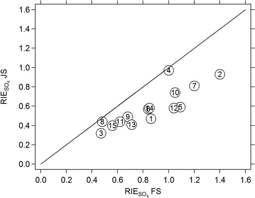
The median NO₃ and SO₄ values are compared with the NO₃ and SO₄ measured by the PILS instrument (Figure 1). Differences in the NO₃ and SO₄ mass concentrations between the PILS and that of the ACSM, may be a result of slightly different size cut (PILS 1.4 μm and ACSM 1 μm). The calibration values determined using both the JS and FS mode calculated using the analysis procedures outlined in the new ACSM acquisition software are listed for each participating instrument in Table S1. A large difference was observed for the RIE for sulfate with an average increase of 48% between the two methods, likely the result of the slower evaporation rate of sulfate particles that are being incorrectly represented in the JS mode (Figure 2).

Figure 1. Time series comparison of the median (a) SO₄, and (b) NO₃ with those values measured by the PILS. The shaded areas represent the 75th and 25th percentiles.

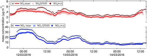
Figure 2. RIE values (left axis) measured using the jump scan mode and the full scan mode. Numbers represent the instrument number (1 through 15).

The inorganic species concentrations for NO₃, NH₄, and SO₄ were compared to the median value calculated for all instruments in order to illustrate the agreement between instruments (Figures S5–S7). An error of 30% has been identified as the standard error for total mass measurements for Aerodyne AMS instruments (Bahreini et al. 2009). Bahreini et al. (2009) calculated an overall uncertainty of 34% for ammonium and nitrate, 36% for sulfate, 38% for organic species. This overall uncertainty includes uncertainties associated with the IE, RIE, and CE. With the exception of one or two instruments, the slopes calculated for each instrument against the median fall between ±30% of the median values.

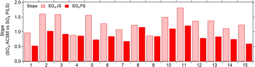
Investigating the agreement of each individual instrument with the PILS-IC SO₄ data for the two different calibration methods (JS vs FS), we observe that the FS calibration method results in an overall decrease in the ACSM SO₄ concentrations relative to the PILS SO₄ (Figure 3). If we calculate the improvement in the variation of the SO₄ mass concentrations using both calibration methods, we observe a decrease in the standard deviation from 1.08 to 0.68 from the JS to the FS methods, respectively. For the remainder of the discussion, we use the calibrations from the FS method.

Figure 3. Slope values, obtained through orthogonal fits, of the ACSM SO₄ concentrations compared with PILS SO₄ concentrations for the JS and FS methods.

Statistical Z-score analysis

To illustrate the agreement between the different instruments in a robust manner, a Z-score calculation was performed on the data following the methods defined by the international standard organization (ISO 5752-2), allowing us to evaluate instrument performance relative to the median of all instruments participating in the intercomparison (Equation (1)(1) $$Z_i=\mathrm{ }\frac{X_i-X^{\mathrm{*}}}{{\sigma }_p}\mathrm{ }$$(1) ). (1) $$Z_i=\mathrm{ }\frac{X_i-X^{\mathrm{*}}}{{\sigma }_p}\mathrm{ }$$(1) where X_i represents the average concentration of each species (i) for a given instrument, and X* and σ_p correspond to the average and standard deviation for that species over all instruments. This approach evaluates if the variations in the different instruments from the reference value fall within a defined criterion. According to this test, instrument performance is considered acceptable when values fall between 2 and −2 (indicated by the green lines in Figure 4) (ISO 5725–51998). Values falling between 2 and 3 indicate that some problems exist.

Figure 4. Z-score values calculated for the 15 participating ACSM instruments for inorganic species.

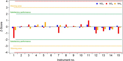
The calculated Z-scores for each of the inorganic species show good agreement, with all instruments within the acceptable range of 2 and −2 (Figure 4). These results demonstrate a considerable improvement over the previous intercomparison exercise (Crenn et al. 2015) which we attribute to the improved calibration procedures. However, larger variabilities are still associated with SO₄ than with the other inorganic species.

During this work, an artifact was identified in relation to the SO₄ signal. During pure ammonium sulfate calibration, the typical m/z for (NH₄)₂SO₄ were observed at 15 (NH⁺), 16 (NH₂⁺), 17 (NH₃⁺), 48 (SO⁺), 64 (SO₂⁺), 80 (SO₃⁺), 81 (HSO₃⁺), and 98(H₂SO4⁺), but a signal was unexpectedly observed for some instruments at m/z 30. The magnitude of this m/z 30 with respect to total measured (NH₄)₂SO₄ ranged from 0.01 to 0.173 and varied inversely to the RIE for SO₄ (Figure 5). The resolution of the Q-ACSM is not sufficient to accurately identify the nature of this peak, and its origin is uncertain. It may be related to sulfate induced surface chemistry on the vaporizer producing NO⁺ and/or organic (e.g., C₂H₆⁺ or CH₂O⁺) fragments. Tests were run to verify that this was not related to impurities in the (NH₄)₂SO₄ solution used for atomization.

Figure 5. SO₄ Artifact observed during (NH₄)₂SO₄ calibration. Numbers represent the instrument number (1 through 15).

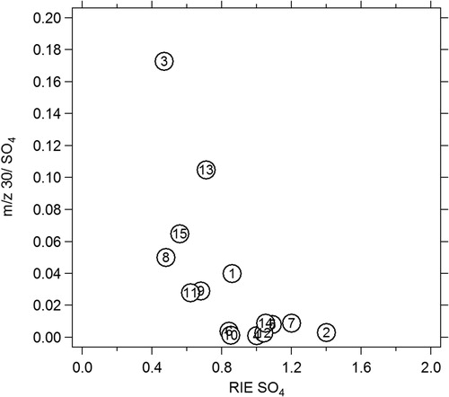
Although, this artifact is relatively limited, it may become significant in periods of high SO₄ concentrations. Further work, notably including high-resolution AMS measurements, are needed to fully understand the nature of this artifact.

Organic aerosol

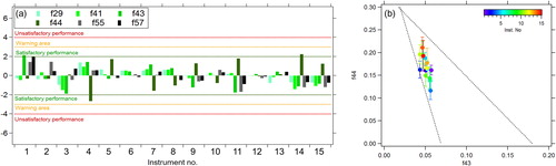
As highlighted by many studies, the organic signal in aerosol mass spectrometers comes from a complex mixture of many different compounds and hence characterizing their sources and properties is difficult. Dedicated calibration and intercomparison exercises can improve our understanding of the instrument response to these organic species. During previous intercomparison and laboratory studies, comparisons of the organic mass loading measured by different ACSM instruments showed a considerable variability as did the fraction of the organic signal at specific m/z values (Crenn et al. 2015). Comparing the individual instrument organic mass loading measurements to the median of the ACSM organic measurements calculated using the default fragmentation table in this dataset, we observe slopes from 0.63 to 1.24 (Figure S8). To determine if particular m/z values in the organic spectra showed more variation than others, the Z-score for the fractions of the prominent organic fragments, f₂₉ (fraction of m/z 29 to the total OA signal), f₄₃ (fraction of m/z 43 to the total OA signal), f₄₄ (fraction of m/z 44 to the total OA signal), f₅₅ (fraction of m/z 55 to the total OA signal), and f₅₇ (fraction of m/z 57 to the total OA signal) were calculated. These masses were chosen as they are often responsible for the majority of mass in the ambient organic signal (Fröhlich et al. 2015b), and are marker peaks representing the extent of oxidation of the OA. Similar to Fröhlich et al. (2015b) and Crenn et al. (2015), we observe the largest variability in the organic fragments at m/z 44 (Figure 6a), with four instruments having Z-scores outside the acceptable range.

Figure 6. (a) Z-score analysis of the prominent organic fragments calculated with respect to the median values for all 15 instruments over the entire campaign. (b) Plot of f₄₄ vs f₄₃ for all instruments that took part in the intercomparison. The dashed lines are from Ng et al. (2010) for ambient measurements.

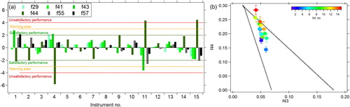
The plot of f₄₄ vs f₄₃ in Figure 6b shows that although the f₄₃ values do not vary by more than ±0.02, the f₄₄ values range from 0.15 to 0.30 for measurements taken over the same three-day period. Fröhlich et al. (2015b) emphasized that this large variability in f₄₄ does not affect the resulting factors identified using positive matrix factorization, but it does highlight the need to understand how organic aerosol components are detected by these instruments. Much of the variability in f₄₄ is thought to be due to an instrument artifact (Pieber et al. 2016) where the existence of carbonaceous material on the vaporizer can affect both the desorption and decomposition process of NO_3, and reactions at the vaporizer surface. These reactions can generate CO₂ with C from the carbonaceous deposits and O from the NO, NO₂, and HNO₃ thermal decomposition products of NH₄NO₃, and hence increase the m/z 44 signal which is then erroneously attributed to organic aerosol. The artifact can be quantified in each instrument by determining the ratio of m/z 44/NO₃ during calibrations using pure AN. During this ILC exercise, 15 Q-ACSM instruments were operated side-by-side, providing us with a unique possibility to quantify this artifact, and to evaluate how it varies among 15 instruments of the same type. The resulting m/z 44/NO₃ ranged from values of 0.01 to 0.26 (Figure 7), similar to those reported in Pieber et al. (2016). As also observed by Pieber et al. (2016), the m/z 44/NO₃ tends to increase with increasing m/z 30/m/z 46 (NO⁺/NO₂⁺) ratio from pure AN (Figure 8). Instruments are numbered (and hence colored) as a function of artifact, therefore in Figure 6b, those f₄₄ data points colored in blue are those with the lowest artifact value, and may best represent the real f₄₄ for ambient organic aerosol during this measurement period.

Figure 7. Ratio of m/z 44/NO₃, as well as the NO₃ 30/46 ratio for each of the instruments that participated in the comparison. The color represents the intensity of the m/z 44/NO₃ (left y-axis) artifact and is the same throughout the manuscript.

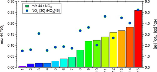
Figure 8. The m/z 44/NO₃ artifact as a function of NO₃_MF for the ACSM instruments. The error bars represent ±1σ.

Application of fragmentation table corrections

Pieber et al. (2016) suggested a fragmentation table correction that can be applied to each individual instrument in order to correct for this artifact (Equation (2)(2) $$\text{frag}\_\text{organic}\left[44\right]= 44,-\text{frag}\_\text{air}\left[44\right],-\mathrm{b}*1.05*\text{frag}\_\text{nitrate}\left[30\right],-\mathrm{b}*1.05*\text{frag}\_\text{nitrate}\left[46\right]$$(2) ): (2) $$\text{frag}\_\text{organic}\left[44\right]= 44,-\text{frag}\_\text{air}\left[44\right],-\mathrm{b}*1.05*\text{frag}\_\text{nitrate}\left[30\right],-\mathrm{b}*1.05*\text{frag}\_\text{nitrate}\left[46\right]$$(2) where frag_organic[44] corresponds to the instrument signal at m/z 44 that is attributed to organic aerosol, frag_air[44] is the signal at m/z 44 that is attributed to the air signal, frag_nitrate[30] and frag_nitrate[46] correspond to the signals at m/z 30 and 46 that are attributed to nitrate aerosol. The value “b” corresponds to the ratio of m/z 44/NO₃ measured during calibration (Figure 7). The factor of 1.05 is due to the difference between NO₃ (calculated via the frag table and used to determine the b value) and the sum of the signals at m/z 30 and m/z 46. Since m/z 44 is the major fragment in aged organic aerosol, such as measured in this intercomparison, and nitrate loadings are high in this dataset, applying this correction impacts total organic mass loading as well as m/z 44 and thus the ratios for each fragment.

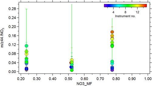
Applying the correction based on Equation (2)(2) $$\text{frag}\_\text{organic}\left[44\right]= 44,-\text{frag}\_\text{air}\left[44\right],-\mathrm{b}*1.05*\text{frag}\_\text{nitrate}\left[30\right],-\mathrm{b}*1.05*\text{frag}\_\text{nitrate}\left[46\right]$$(2) , led to an increase in the scatter of the f₄₄ vs f₄₃ plot between the different instruments, but also for a given instrument (represented by the error bars in Figure S10b) and worse agreement with the mean (Z-scores in Figure S10a). This correction assumes the magnitude of the artifact is independent of chemical composition, basing the correction on measurements made with pure NH₄NO₃. During this intercomparison we performed calibrations at variable nitrate mass fractions (NO₃_MF) using mixtures of NH₄NO₃ and (NH₄)₂SO₄, and from this data we observe that the magnitude of the artifact varies as a function of NO₃_MF (Figure 8).

For instruments with large artifacts there is a significant increase between NO₃_MF = 0.52 and NO₃_MF = 0.78 (pure NH₄NO₃). Note that in the atmosphere, while NO₃_MF can occasionally exceed 50% contribution, it almost never accounts for more than 80% of the measured PM₁ concentrations (Zhang et al. 2007). We hypothesize that this artifact measured in the ACSM instruments at pure ammonium nitrate mass fractions may not be representative of ambient conditions and utilize the mixture data to test that hypothesis by applying a correction based on Equation (2)(2) $$\text{frag}\_\text{organic}\left[44\right]= 44,-\text{frag}\_\text{air}\left[44\right],-\mathrm{b}*1.05*\text{frag}\_\text{nitrate}\left[30\right],-\mathrm{b}*1.05*\text{frag}\_\text{nitrate}\left[46\right]$$(2) where b is a time varying value based on the measured ambient NO₃_MF. The time dependent correction was applied manually to frag_organic[44], but the capability to perform this correction automatically through the fragmentation table will be included in future versions of the ACSM analysis software. Because there was reasonable agreement between the two lowest NO₃_MF points in Figure 9 for a given instrument, if ambient NO₃_MF was less than 0.5, then b was taken to be the average of these. For points with NO₃_MF between 0.5 and 0.8, a linear fit between the two highest NO3_MF points was used.

Figure 9. (a) Z-scores of the prominent organic fragments and (b) average f₄₄ vs f₄₃ concentrations for all participating instruments with the fragmentation table correction applied.

Figure 9 shows that applying this correction significantly reduces the variability in the organic fragment ions, with nearly all peaks falling within the −2 and 2 lines of the Z-score plots, and that the observed variability in the average f₄₄ also decreases. However, the differences in the f₄₄ between instruments are still significant, with ranges from 0.11 to 0.21.

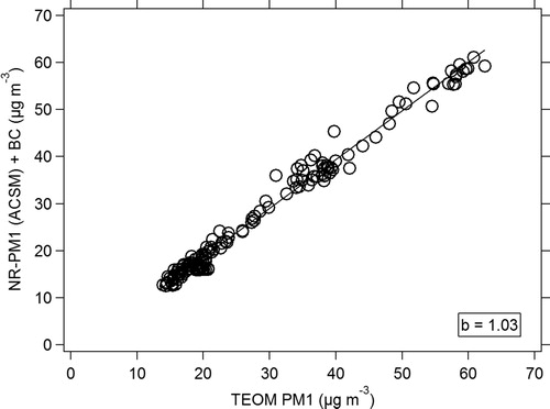
The agreement in total organic mass against the median concentrations also improved with slope values ranging from 0.75 up to 1.21 (Figure S11). Continuing work on OA measurement artifacts and uncertainties should be addressed in future intensive laboratory studies. Combining this new m/z 44 artifact correction along with the new calibration procedures, we obtain a submicron mass concentration that compares well with collocated PM₁ measurements (Figure 10).

Figure 10. ACSM median NR-PM₁ concentrations + BC measurements compared to the total PM₁ mass measured by the TEOM. The fit is an orthogonal fit, not forced through 0.

Conclusions

This work presents measurements during the 2016 Q-ACSM instrument intercomparison at the Aerosol Chemical Monitor Calibration Centre (ACMCC), located at the SIRTA site south-west of Paris. This exercise is a continuation of the first intercomparison exercise that took place as part of ACTRIS 1 (Crenn et al. 2015; Fröhlich et al. 2015b) and provided the opportunity to perform tests with new calibration protocols for the Q-ACSM instruments. Within these tests, calibrations were performed with the same sampling protocol as during ambient sampling, ensuring that data is acquired and analyzed under the same operating conditions used during measurements. Results showed that the use of full-scan mode calibration data (as opposed to jump-scan mode data) improved the comparison of SO₄ mass loading with external data and improved the correlation of the measured SO₄ mass concentrations among the 15 instruments, with the standard deviation decreasing from 1.08 to 0.68. Based on these results, full-scan mode calibration protocols are recommended by the manufacturer as well as within the ACTRIS standard operating procedures. These results illustrate that these instruments have good comparability and are within the ±30% uncertainty range recommended for these instruments. This uncertainty range should always be considered when comparing these instruments to other co-located instruments. These intercomparison exercises illustrates that ACSM data is highly valuable for future atmospheric model evaluation and development.

In addition, the new calibration procedures have the added advantage of acquiring a full mass spectrum providing each user the opportunity to assess and quantify the presence of instrument artifacts, notably the m/z 44 artifact. Applying the m/z artifact correction following Pieber et al. (2016) increased the variability in both the measured f₄₄ and the total organic mass loading. Moreover, in cases of high artifact values (m/z 44/NO₃ > 0.10) the fragmentation table adjustment as per Pieber et al. (2016), results in sometimes unrealistically low f₄₄ values. In ambient air, NO₃ mass fraction (NO₃_MF) may occasionally exceed 0.5 but rarely reaches 0.8. An alternative correction, accounting for varying NO₃_MF, was tested. Application of this alternative correction resulted in significant improvements in the f₄₄ reproducibility, as well as for other dominant organic fragments, leading to an improvement in the agreement of the total measured organic mass concentrations over all instruments. The analysis and interpretation of ACSM data, especially related to the organic spectra, are constantly evolving, as is our knowledge of the instrument response to different chemical species (Hu et al. 2017; Pieber et al. 2016). It is possible that the high fractions of measured nitrate during this intercomparison were in part due to the presence of organic nitrates (Kiendler-Scharr et al. 2016). Given the spatial distribution of ACSM instruments in Europe and the continuous sampling nature of the ACSM measurements, understanding how the instruments respond to different organics species, including organic nitrates, is essential, and will be the focus of future intercomparison exercises.

Acknowledgment

We would like to say a special thanks to JL Jimenez for fruitful discussions on the m/z 44 artifact correction as a function of NO₃_MF.

Funding

This project has received funding from the European Union's Horizon 2020 research and innovation programme under grant agreement No 654109.

The US Department of Energy Small Business Innovative Research program (award number DE-SC0017041) provided support for development of ACSM calibration procedures. CNRS, CEA, and INERIS are acknowledged for financial support of the ACMCC. The intercomparison campaign and the following data treatment have been conducted in collaboration with the French reference laboratory for air quality monitoring (LCSQA), funded by the French Ministry of Environment. COST action CA16109 Chemical On-Line cOmpoSition and Source Apportionment of fine aerosoLs COLOSSAL grant is gratefully acknowledged for the support of data workshops. M.C. Minguillón acknowledges the Ramón y Cajal fellowship awarded by the Spanish Ministry of Economy, Industry and Competitiveness. The CIEMAT participation has been partially funded by MINECO/AEI/FEDER, UE (CGL2017-85344-R and CGL2017-90884-REDT) and TIGAS-CM (Y2018/EMT-5177) Project. PSI is grateful for financial support by the Federal Office for the Environment in Switzerland.

References

- Allan, J. D., A. E. Delia, H. Coe, K. N. Bower, M. R. Alfarra, J. L. Jimenez, A. M. Middlebrook, F. Drewnick, T. B. Onasch, M. R. Canagaratna, et al. 2004. A generalised method for the extraction of chemically resolved mass spectra from aerodyne aerosol mass spectrometer data. J. Aerosol Sci. 35 (7):909–22. doi:10.1016/j.jaerosci.2004.02.007.
- Bahreini, R., B. Ervens, A. Middlebrook, C. Warneke, J. D. Gouw, P. DeCarlo, J. Jimenez, C. Brock, J. Neuman, and T. Ryerson. 2009. Organic aerosol formation in urban and Industrial plumes near Houston and Dallas, Texas. J. Geophys. Res. Atmos. 114:D00F16. doi:10.1029/2008JD011493.
- Bessagnet, B., G. Pirovano, M. Mircea, C. Cuvelier, A. Aulinger, G. Calori, G. Ciarelli, A. Manders, R. Stern, S. Tsyro, et al. 2016. Presentation of the EURODELTA III intercomparison exercise – Evaluation of the chemistry transport models' performance on criteria pollutants and joint analysis with meteorology. Atmos. Chem. Phys. 16 (19):12667–701. doi:10.5194/acp-16-12667-2016.
- Budisulistiorini, S. H., M. R. Canagaratna, P. L. Croteau, K. Baumann, E. S. Edgerton, M. S. Kollman, N. L. Ng, V. Verma, S. L. Shaw, E. M. Knipping, et al. 2014. Intercomparison of an aerosol chemical speciation monitor (ACSM) with ambient fine aerosol measurements in downtown Atlanta, Georgia. Atmos. Meas. Tech. 7 (7):1929–41. doi:10.5194/amt-7-1929-2014.
- Canagaratna, M. R., J. T. Jayne, J. L. Jimenez, J. D. Allan, M. R. Alfarra, Q. Zhang, T. B. Onasch, F. Drewnick, H. Coe, A. Middlebrook, et al. 2007. Chemical and microphysical characterization of ambient aerosols with the aerodyne aerosol mass spectrometer. Mass Spectrom. Rev. 26 (2):185–222. doi:10.1002/mas.20115.
- Cavalli, F., M. Viana, K. E. Yttri, J. Genberg, and J.-P. Putaud. 2010. Toward a standardised thermal-optical protocol for measuring atmospheric organic and elemental carbon: The EUSAAR protocol. Atmos. Meas. Tech. 3 (1):79–89. doi:10.5194/amt-3-79-2010.
- Ciarelli, G., S. Aksoyoglu, I. El Haddad, E. A. Bruns, M. Crippa, L. Poulain, M. Äijälä, S. Carbone, E. Freney, C. O’Dowd, et al. 2017. Modelling winter organic aerosol at the European scale with CAMx: Evaluation and source apportionment with a VBS parameterization based on novel wood burning smog chamber experiments. Atmos. Chem. Phys. 17 (12):7653–69. doi:10.5194/acp-17-7653-2017.
- Crenn, V., J. Sciare, P. L. Croteau, S. Verlhac, R. Fröhlich, C. A. Belis, W. Aas, M. Äijälä, A. Alastuey, B. Artiñano, et al. 2015. ACTRIS ACSM intercomparison – Part 1: Reproducibility of concentration and fragment results from 13 individual quadrupole aerosol chemical speciation monitors (Q-ACSM) and consistency with co-located instruments. Atmos. Meas. Tech. 8 (12):5063–87. doi:10.5194/amt-8-5063-2015.
- Fröhlich, R., M. J. Cubison, J. G. Slowik, N. Bukowiecki, F. Canonaco, P. L. Croteau, M. Gysel, S. Henne, E. Herrmann, J. T. Jayne, et al. 2015a. Fourteen months of on-line measurements of the non-refractory submicron aerosol at the Jungfraujoch (3580 m a.s.l.) – Chemical composition, origins and organic aerosol sources. Atmos. Chem. Phys. 15 (19):11373–398. doi:10.5194/acp-15-11373-2015.
- Fröhlich, R., V. Crenn, A. Setyan, C. A. Belis, F. Canonaco, O. Favez, V. Riffault, J. G. Slowik, W. Aas, M. Aijälä, et al. 2015b. ACTRIS ACSM intercomparison – Part 2: Intercomparison of ME-2 organic source apportionment results from 15 individual, co-located aerosol mass spectrometers. Atmos. Meas. Tech. 8 (6):2555–76. doi:10.5194/amt-8-2555-2015.
- Fröhlich, R., M. J. Cubison, J. G. Slowik, N. Bukowiecki, A. S. H. Prévôt, U. Baltensperger, J. Schneider, J. R. Kimmel, M. Gonin, U. Rohner, et al. 2013. The ToF-ACSM: A portable aerosol chemical speciation monitor with TOFMS detection. Atmos. Meas. Tech. 6 (11):3225–41. doi:10.5194/amt-6-3225-2013.
- Hari, P., and Kulmala, M. 2005. Station for measuring ecosystem-atmosphere relations (SMEAR II). Boreal Environ. Res. 10:315–22.
- Hu, W., P. Campuzano-Jost, D. A. Day, P. L. Croteau, M. R. Canagaratna, J. T. Jayne, D. R. Worsnop, and J. L. Jimenez. 2017. Evaluation of the new capture vaporizer for aerosol mass spectrometers (AMS) through field studies of inorganic species. Aerosol Sci. Technol. 51 (6):735–54. doi:10.1080/02786826.2017.1296104.
- ISO, 5725-5. 1998. Accuracy (trueness and precision) of measurement methods and results – Part 5: Alternative methods for the determination of the precision of a standard measurement method. Geneva: International Organization for Standardization.
- Kiendler‐Scharr, A., A. A. Mensah, E. Friese, D. Topping, E. Nemitz, A. S. H. Prevot, M. Äijälä, J. Allan, F. Canonaco, R. R. Canagaratna, et al. 2016. Ubiquity of organic nitrates from nighttime chemistry in the European submicron aerosol. Geophys. Res. Lett. 43:7735–44. doi:10.1002/2016GL069239.
- Liu, P. S. K., R. Deng, K. A. Smith, L. R. Williams, J. T. Jayne, M. R. Canagaratna, K. Moore, T. B. Onasch, D. R. Worsnop, and T. Deshler. 2007. Transmission efficiency of an aerodynamic focusing lens system: Comparison of model calculations and laboratory measurements for the aerodyne aerosol mass spectrometer. Aerosol Sci. Technol. 41 (8):721–33. doi:10.1080/02786820701422278.
- Middlebrook, A. M., R. Bahreini, J. L. Jimenez, and M. R. Canagaratna. 2012. Evaluation of composition-dependent collection efficiencies for the aerodyne aerosol mass spectrometer using field data. Aerosol Sci. Technol. 46 (3):258–71. doi:10.1080/02786826.2011.620041.
- Ng, N. L., M. R. Canagaratna, Q. Zhang, J. L. Jimenez, J. Tian, I. M. Ulbrich, J. H. Kroll, K. S. Docherty, P. S. Chhabra, R. Bahreini, et al. 2010. Organic aerosol components observed in Northern hemispheric datasets from aerosol mass spectrometry. Atmos. Chem. Phys. 10 (10):4625–41. doi:10.5194/acp-10-4625-2010.
- Ng, N. L., S. C. Herndon, A. Trimborn, M. R. Canagaratna, P. L. Croteau, T. B. Onasch, D. Sueper, D. R. Worsnop, Q. Zhang, Y. L. Sun, et al. 2011. An aerosol chemical speciation monitor (ACSM) for routine monitoring of the composition and mass concentrations of ambient aerosol. Aerosol Si. Technol. 45 (7):780–94. doi:10.1080/02786826.2011.560211.
- O’Connor, T., S. Jennings, and C. O’Dowd. 2008. Highlights of fifty years of atmospheric aerosol research at mace head. Atmos. Res. 90:338–55. doi:10.1016/j.atmosres.2008.08.014.
- Olfert, J., and N. Collings. 2005. New method for particle mass classification—The Couette centrifugal particle mass analyzer. J. Aerosol Sci. 36 (11):1338–52. doi:10.1016/j.jaerosci.2005.03.006.
- Petit, J.-E., O. Favez, A. Albinet, and F. Canonaco. 2017. A user-friendly tool for comprehensive evaluation of the geographical origins of atmospheric pollution: Wind and trajectory analyses. Environ. Model. Softw. 88:183–87. doi:10.1016/j.envsoft.2016.11.022.
- Petit, J.-E., O. Favez, J. Sciare, V. Crenn, R. Sarda-Estève, N. Bonnaire, G. Močnik, J. C. Dupont, M. Haeffelin, and E. Leoz-Garziandia. 2015. Two years of near real-time chemical composition of submicron aerosols in the region of Paris using an aerosol chemical speciation monitor (ACSM) and a multi-wavelength Aethalometer. Atmos. Chem. Phys. 15 (6):2985–3005. doi:10.5194/acp-15-2985-2015.
- Pieber, S. M., I. El Haddad, J. G. Slowik, M. R. Canagaratna, J. T. Jayne, S. M. Platt, C. Bozzetti, K. R. Daellenbach, R. Fröhlich, A. Vlachou, et al. 2016. Inorganic salt interference on CO2+ in aerodyne AMS and ACSM organic aerosol composition studies. Environ. Sci. Technol. 50 (19):10494–503. doi:10.1021/acs.est.6b01035.
- Ripoll, A., M. C. Minguillón, J. Pey, J. L. Jimenez, D. A. Day, Y. Sosedova, F. Canonaco, A. S. H. Prévôt, X. Querol, and A. Alastuey. 2015. Long-term real-time chemical characterization of submicron aerosols at Montsec (Southern Pyrenees, 1570 m a.s.l.). Atmos. Chem. Phys. 15 (6):2935–51. doi:10.5194/acp-15-2935-2015.
- Sciare, J., O. d’Argouges, R. Sarda‐Estève, C. Gaimoz, C. Dolgorouky, N. Bonnaire, O. Favez, B. Bonsang, and V. Gros. 2011. Large contribution of water‐insoluble secondary organic aerosols in the region of Paris (France) during wintertime. J. Geophys. Res. Atmos. 116(D22): D22203. doi:10.1029/2011JD015756, 2011
- Stein, A. F., R. R. Draxler, G. D. Rolph, B. J. B. Stunder, M. D. Cohen, and F. Ngan. 2015. NOAA’s HYSPLIT atmospheric transport and dispersion modeling system. Bull. Amer. Meteorol. Soc. 96 (12):2059–77. doi:10.1175/BAMS-D-14-00110.1.
- Xu, W., P. L. Croteau, L. Williams, M. R. Canagaratna, T. Onasch, E. Cross, X. Zhang, W. Robinson, D. Worsnop, and J. T. Jayne. 2017. Laboratory characterization of an aerosol chemical speciation monitor with PM2. 5 measurement capability. Aerosol Sci. Technol. 51 (1):69–83. doi:10.1080/02786826.2016.1241859.
- Xu, W., A. Lambe, P. Silva, W. Hu, T. Onasch, L. Williams, P. Croteau, X. Zhang, and L. Renbaum-Wolff. 2018. Laboratory evaluation of species-dependent relative ionization efficiencies in the aerodyne aerosol mass spectrometer. Aerosol. Sci. Technol. 52:626–41. doi:10.1080/02786826.2018.1439570.
- Zhang, Q., J. L. Jimenez, M. R. Canagaratna, J. D. Allan, H. Coe, I. Ulbrich, M. R. Alfarra, A. Takami, A. M. Middlebrook, Y. L. Sun, et al. 2007. Ubiquity and dominance of oxygenated species in organic aerosols in anthropogenically-influenced northern Hemisphere midlatitudes, 2007. Geophys. Res. Lett. 34:L13801. doi:10.1029/2007GL029979.
- Zhang, Y., L. Tang, P. L. Croteau, O. Favez, Y. Sun, M. R. Canagaratna, Z. Wang, F. Couvidat, A. Albinet, H. Zhang, et al. 2017. Field characterization of the PM2.5 aerosol chemical speciation monitor: Insights into the composition, sources, and processes of fine particles in Eastern China. Atmos. Chem. Phys. 17 (23):14501–17. doi:10.5194/acp-17-14501-2017.