Ionization efficiency of evolved gas molecules from aerosol particles in a thermal desorption aerosol mass spectrometer: Numerical simulations

Abstract

Thermal desorption aerosol mass spectrometers (TDAMSs) with electron ionization are widely used to quantitatively measure aerosol chemical compositions. The physical and chemical mechanisms affecting the ionization efficiency of evolved gas molecules are not fully understood. We have developed a numerical model for simulating the dynamics of gas molecules evolved from aerosol particles. The simulation model is composed of two main sections. The first section simulates the elastic collisions of the evolved gas molecules in a small region near the vaporization source (collision domain), where the mean free paths of the molecules are much shorter than those in the surrounding high vacuum environment. The second section simulates the free-molecular dynamics from the boundary of the first section to the ionizer. The ionization efficiencies of ammonia and hydrogen iodide molecules that evolved from ammonium iodide particles were evaluated. Our results suggest that the molecular collisions during the early stage of plume expansion and possible changes in the molecular velocities induced by these collisions could be an important mechanism affecting the observed variability in the ionization efficiency. However, the physical and chemical processes of the vaporization and ionization of aerosol particles in TDAMSs may be too complex to be quantitatively reproduced using simplified numerical models.

Copyright © 2019 American Association for Aerosol Research

EDITOR:

• Paul Ziemann

1. Introduction

Thermal desorption aerosol mass spectrometers (TDAMSs), including the Aerodyne aerosol mass spectrometer (AMS; Jayne et al. 2000), aerosol chemical speciation monitor (Ng et al. 2011), and particle trap laser desorption mass spectrometer (PT-LDMS; Takegawa et al. 2012), can provide online quantitative analysis of the chemical composition of nonrefractory aerosols. AMS instruments are widely used for field and laboratory studies (e.g., Zhang et al. 2007). The Aerodyne AMS employs flash vaporization of aerosol particles on a heated tungsten surface, followed by electron ionization mass spectrometry. The PT-LDMS employs a carbon dioxide (CO₂) laser (10.6 μm wavelength) to vaporize the aerosol particles collected on a custom-made particle trap. This vaporization mechanism includes both direct heating of the aerosol particles via light absorption and thermal conduction from the heated surface of the particle trap.

Uchida et al. (2019) used a custom-made TDAMS (a modified version of the PT-LDMS) for laboratory experiments, and suggested that the angular distributions of evolved gas molecules can vary for different chemical species. Variability in the angular distributions may affect the overlap of gas plumes and electrons in an ionizer. Uchida et al. (2019) suggested the potential importance of molecular collisions during the initial stage of plume expansion. The purpose of the present study is to investigate the effects of molecular collisions on the TDAMS ionization efficiency based on numerical simulations.

2. Method

2.1. Vaporization sources

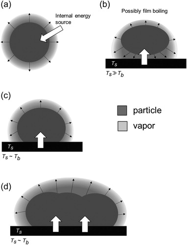
First, we consider the possible TDAMS vaporization mechanisms of aerosol particles. For simplicity, we only consider the boiling (or sublimation) of a single compound, with four types of vaporization mechanisms illustrated in Figure 1. Figure 1a represents the vaporization of an airborne particle induced by an internal energy source, such as laser heating. Figure 1b represents the vaporization of a particle via impaction onto a heated surface. When the surface temperature, T_s, is much higher than the boiling point of the aerosol compound, T_b, the bottom part of the particle can be immediately vaporized, with a thin layer of vapor potentially forming between the particle and hot surface (film boiling). This process may occur during flash vaporization on an AMS vaporizer. Figure 1c and d represent a single particle and ensemble of particles, respectively, collected on a surface. The surface is heated by an external energy source after particle collection. If T_s exceeds T_b, particle vaporization can proceed rapidly, with this process corresponding to laser-induced heating of the particle trap in the PT-LDMS.

Figure 1. Potential vaporization mechanisms in TDAMSs. (a) Vaporization of an airborne particle induced by an internal energy source. (b) Vaporization of a particle via impaction onto a heated surface. Vaporization of (c) a single particle and (d) an ensemble of particles, respectively, collected on a surface.

2.2. Model description

Previous studies have described a direct simulation Monte Carlo (DSMC) method for simulating molecular collisions under reduced pressure conditions (Bird 1994; Nanbu 1980; Nanbu et al. 2000; Yasuhara and Daiguji 1992). The derivation of the equations employed in the present numerical simulations is based on the method described in Nanbu et al. (2000) and Yasuhara and Daiguji (1992). Although a molecular dynamics (MD) method could also be used to simulate gas-particle interactions (e.g., Takahama and Russell 2011), we do not use a MD method because the computational costs would become very high in our simulation conditions (molecular number ∼10⁹; spatial scale > μm).

Here, we consider two species (A and B) evaporating from particles in a TDAMS. We set the numbers of A and B molecules equal to each other, and conserve them throughout the simulation (i.e., no chemical reaction). The initial condition assumes that an ensemble of molecules containing equal numbers of A and B is located at the vaporization source (z = 0 plane). The velocities of the gas molecules that evolved from the source are calculated based on the Maxwell–Boltzmann distribution. The velocity distribution function, $f_{c_p},$ is expressed as: (1) $$f_{c_p}={\left(\frac{m}{2\pi \mathit{kT}}\right)}^{1/2}\exp \left(-\frac{m{c}_p^2}{2kT}\right)\mathrm{}(p=x,y,z),\mathrm{}$$(1) where m is the mass of a gas molecule, k is the Boltzmann constant, T is the temperature, and c_p is the p-th component of the initial molecular velocity, which is given by: (2) $$c_x=\sqrt{-\frac{2kT}{m}\mathrm{l}\mathrm{n}\left(U_1\right)}\times \text{cos}\left(2\pi U_2\right)\mathrm{}$$(2) (3) $$c_y=\sqrt{-\frac{2kT}{m}\mathrm{l}\mathrm{n}\left(U_1\right)}\times \text{sin}\left(2\pi U_2\right)\mathrm{}$$(3) (4) $$c_z=\left|\sqrt{-\frac{2kT}{m}\ln \left(U_3\right)}\times \text{cos}\left(2\pi U_4\right)\right|\mathrm{}$$(4) where U₁, U₂, U₃, and U₄ are uniform random numbers (0 < U₁, U₂, U₃, U₄ < 1) (Yasuhara and Daiguji 1992). We consider only $c_z\ge 0$ for our simulations because the z = 0 plane is set as the vaporizer surface. When the evolved gas molecules intersect the z = 0 plane, these molecules are released at velocities determined by Lambert’s cosine law. The online supplementary information (SI) gives further details on the derivation of the above equations.

The simulation model is composed of two main sections. The first section simulates the elastic collisions of the evolved gas molecules assuming that all collisions are binary collisions. The second section simulates the free-molecular dynamics from the boundary of the first section to the TDAMS ionizer.

The first section defines the initial key region of the proposed model. We consider the elastic collisions of the gas molecules in a small region near the vaporization source, where the mean free paths of the molecules are shorter than those in the surrounding high vacuum environment. Figure 2a conceptually illustrates the structure of the first section of the model. We assume that the gas molecule collisions only occur in a small micrometer-scale region (hereafter referred to as the collision domain). The collision domain is composed of cubic grid cells that are arranged along the x, y, and z axes. The center of the vaporization source is set at the origin of the xyz coordinate system. The translational displacements and molecular collisions during a simulation time step, Δt, are calculated separately. The molecule positions at time t + Δt are determined using the translational displacements calculated from the molecular velocities and Δt. The grid cell is used for the diagnostics of the molecular collisions and does not limit the spatial resolution of the individual molecule positions. In general DSMC simulations, the grid cell size is set approximately equal to the mean free path of molecules. The basic assumption is the spatial distribution of molecules is uniform in a grid cell, such that the behavior of a large number of molecules can be represented by the probabilistic treatment of a small number of sample molecules. The SI gives further details of the sample molecules and weighting factor.

Figure 2. (a) Conceptual structure of the first section (collision domain) of the model. The collision domain is composed of cubic grid cells that are arranged along the x, y, and z axes. The center of the vaporization source is set at the origin of the xyz coordinate system. (b) Conceptual illustration of the collision between the i-th and j-th molecules in a grid cell. The ratio of the relative velocity ($g_{\mathit{ij}}$) to the maximum relative velocity ($g_{\max }$) represents the probability of the collision between two selected molecules. The probability of collisions becomes larger as $g_{\mathit{ij}}$ approaches $g_{\max }.$

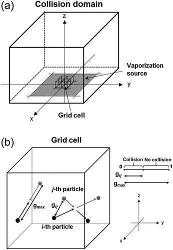
The mean free path of A molecules in a binary mixture of A and B molecules is given by (Seinfeld and Pandis 2006): (5) $${\lambda }_{\mathrm{AB}}=\frac{1}{\sqrt{2}\pi n_{\mathrm{A}}{d}_{\mathrm{A}}^2+\pi \sqrt{1+\frac{{\mathit{MW}}_{\mathrm{A}}}{{\mathit{MW}}_{\mathrm{B}}}}{n}_{\mathrm{B}}{d}_{\mathrm{AB}}^2}\mathrm{}$$(5) and the mean free path of B molecules in a binary mixture of A and B molecules is given by: (6) $${\lambda }_{\mathrm{BA}}=\frac{1}{\sqrt{2}\pi n_{\mathrm{B}}{d}_{\mathrm{B}}^2+\pi \sqrt{1+\frac{{\mathit{MW}}_{\mathrm{B}}}{{\mathit{MW}}_{\mathrm{A}}}}{n}_{\mathrm{A}}{d}_{\mathrm{AB}}^2}\mathrm{}$$(6) where n_A and n_B are the number concentrations of A and B molecules, respectively, in each cell, MW_A and MW_B are the molecular weights of A and B, respectively, and d_A, d_B, and d_AB are the collision diameters for the A + A, B + B, and A + B binary collisions, respectively.

The diagnostic calculations of molecular collisions are performed individually for A + A, B + B, and A + B. For simplicity, we collectively describe the three types of collisions in the following paragraphs. The number of molecular collisions (N_col) in each grid cell is calculated via the following equation (Nanbu et al. 2000; Yasuhara and Daiguji 1992): (7) $$N_{\mathrm{col}}=\frac{1}{2N}n\sigma \Delta t\sum _i^N\sum _j^N{g}_{\mathit{ij}},$$(7) where N is the number of sample molecules in each cell, n is the number concentration of molecules in each cell, σ is the collisional cross section, and $g_{\mathit{ij}}$ is the relative velocity between the i-th and j-th molecules. If we consider the A + A collisions, for example, N is the number of A, n is the number concentration of A, and σ is the collisional cross section for A + A.

Here, $g_{\mathit{ij}}$ is replaced with the maximum relative velocity, $g_{\max },$ to improve the efficiency of the computational calculations. We set $g_{\max }$ as twice the mean thermal velocity. The maximum number of molecular collisions is given by (Nanbu et al. 2000; Yasuhara and Daiguji 1992): (8) $$N_{\max }=\frac{1}{2}\left(N-1\right)n\sigma g_{\max }\Delta t.$$(8)

A collision between two randomly selected molecules is repeated N_max times in each grid cell. However, there could be substantial uncertainties in estimating the maximum number of collisions in a given grid cell when n is very low. The SI gives further details of the diagnostics of molecular collisions at low concentrations.

It is obvious from the above-mentioned definition that N_max overestimates the actual number of collisions. We correct for this overestimation by assuming that the collision between the randomly selected i-th and j-th molecules only occurs if the ratio of $g_{\mathit{ij}}$ to $g_{\max }$ is larger than a uniform random number, U (0 < U < 1) (Nanbu et al. 2000; Yasuhara and Daiguji 1992). Figure 2b illustrates the collision between the i-th and j-th molecules in a grid cell. The ratio of $g_{\mathit{ij}}$ to $g_{\max }$ represents the probability of the collision between two selected molecules, with the probability increasing as $g_{\mathit{ij}}$ approaches $g_{\max }.$ The molecular velocities after a collision are derived from the laws of conservation of momentum and energy: (9) $$c_{i,p}^{,}=\left(\frac{{m_{i}c}_{i,p}+{m_{j}c}_{j,p}}{m_i+m_j}\right)-\frac{m_j{g}_{\mathit{ij}}}{m_i+m_j}{R}_p,$$(9) (10) $$c_{j,p}^{,}=\left(\frac{{m_{i}c}_{i,p}+{m_{j}c}_{j,p}}{m_i+m_j}\right)+\frac{m_i{g}_{\mathit{ij}}}{m_i+m_j}{R}_p,$$(10) (11) $$g_{\mathit{ij}}=\sqrt{{\left(c_{j,x}-c_{i,x}\right)}^2+{\left(c_{j,y}-c_{i,y}\right)}^2+{\left(c_{j,z}-c_{i,z}\right)}^2},$$(11) where m_i and m_j are the masses of the i-th and j-th molecules respectively, $c_{i,p}$ and $c_{j,p}$ are the velocities in the p-component of the i-th and j-th molecules, respectively, before the collision (p = x, y, and z), and $c_{i,p}^{,}$ and $c_{j,p}^{,}$ are the velocities in the p-component of the i-th and j-th molecules, respectively, after the collision, and R_p is a randomly generated unit vector in the p-component (Nanbu et al. 2000; Yasuhara and Daiguji 1992). As mentioned above, the behavior of a large number of molecules can be represented by the probabilistic treatment of a small number of sample molecules. Although the i-th and j-th molecules that were randomly selected by the above procedure may not be located within an actual collision distance, it can be assumed that the grid cell contains another molecule with the same velocity as the j-th molecule that is within the collision distance around the i-th molecule.

The important parameters in the first section of our model include the source profile, time step, grid cell size, and mean free path. These parameters are closely linked with each other, providing a boundary condition for these values. First, we consider molecules A and B individually. Let λ₀ be the mean free path near the vaporization source immediately after the onset of the vaporization (t = Δt). It is expected that λ₀ gives the minimum value of the mean free path in the collision domain if the size of a grid cell is sufficiently small. The value of Δt should be shorter than the mean free time to resolve the molecular collisions, such that: (12) $$\Delta t<\frac{{\lambda }_0}{\overline{c}},$$(12) where $\overline{c}$ is the mean thermal velocity of the gas molecules. Because our simulations are mainly focused on transient processes rather than steady-state processes, the grid cell size should be comparable to the molecular travel distance per time step to maintain a uniform gas density in that grid cell. We define the side length of a grid cell, Δl, as approximately twice the travel distance: (13) $$\frac{\Delta l}{\overline{c}\Delta t}\approx 2.$$(13)

Equation (12)(12) $$\Delta t<\frac{{\lambda }_0}{\overline{c}},$$(12) and $\Delta l/\overline{c}\Delta t=2$ indicate that the upper limit of Δl is 2λ₀. As mentioned above, we calculate λ₀ individually for molecules A and B, and take the smaller value to satisfy the condition. We then calculate Δt (=$\Delta l/2\overline{c}$) individually for molecules A and B, and take the average. The SI gives the details of the calculation.

The second section is similar to the simulation method outlined in Murphy (2016). The boundary condition assumes that the molecular velocities result from the last collision in the first section. The molecular velocities are held constant in the second section. The molecules move to the ionization region via a uniform linear motion, such that the molecular positions at time t + Δt are determined using the translational displacement calculated from the molecular velocities and Δt.

2.3. Laboratory experiments

The full details of the experiment can be found in Uchida et al. (2019). Only the key points relevant to this study are presented here. Polydispersed ammonium iodide (NH₄I) particles were generated using a constant output atomizer (Model 3076, TSI, Inc., USA) and introduced into a custom-made TDAMS. The NH₄I particles that were collected on the particle trap were vaporized using a CO₂ laser (the trap was heated to ∼773 K). We monitored ion signals at mass-to-charge ratio (m/z) of 16 (NH₂⁺), 127 (I⁺), and 128 (HI⁺) originating from ammonia (NH₃) and hydrogen iodide (HI). A quadrupole mass spectrometer (QMS, PrismaPlus, Pfeiffer Vacuum) was used to detect evolved gas molecules. The ion signals were measured by altering the ionizer position relative to the vaporization point. The direction perpendicular to the particle trap plane (normal vector) is set as the polar axis. We defined three positions (a), (b), and (c). The polar angles are 49$°,$ 63$°,$ and 74$°$ for positions (a), (b), and (c), respectively, and the radial distances from the trap to the ionizer are 19, 20, and 23 mm, for positions (a), (b), and (c), respectively.

Because the distance between the particle trap and ionizer was ∼20 mm, we needed relatively high aerosol mass loadings to obtain sufficient ion signals from evolved gas. We introduced aerosol concentrations of ∼20 mg m⁻³ with a flow rate of ∼100 cm³ min⁻¹ and collection time of 10 min, corresponding to ∼8 × 10¹⁶ NH₄I molecules on the trap. We should note that the actual distributions of particles on the surface of the particle trap (three-dimensional mesh structure; Takegawa et al. 2012) are complicated. Since our model can treat simplified source profiles only, it is rather difficult to fully represent the experimental conditions in Uchida et al. (2019). Therefore, the particle distributions were approximated as uniformly deposited areas on a mesh plane of the particle trap. Takegawa et al. (2012) showed that particles are collected on the mesh planes within a ∼3 mm diameter region. A crude calculation shows that the areal molecular density of NH₄I was on the order of 10²¹ m⁻² per mesh plane.

2.4. Simulation setup

We simulated the evolution of NH₃ and HI molecules from NH₄I particles following the experimental setup outlined in Uchida et al. (2019). The number flux of molecules evaporating from the particles, depending on the particle mass and vaporization time scale, could be an important factor affecting the collision frequency. We assume that a constant molecular flux from the source represents the vaporization of a particle or ensemble of particles collected on a surface (Figure 1c and d). The latter would be more appropriate for our case because we introduced relatively high aerosol concentrations in the laboratory.

Saleh et al. (2017) investigated the vaporization time scale in the Aerodyne AMS. The time scale could be largely affected by the balance between the heat transfer from the vaporizer to the particles and the release of latent heat. The vaporizer surface and particles can instantaneously reach an equilibrium at a time scale of <10⁻⁹ s when the heat transfer effect is sufficiently larger than the latent heat effect. Their experimental results yielded an estimated effective heat transfer rate that was two orders of magnitude smaller than that expected from the thermal conductivity of ammonium nitrate. They showed the vaporization time scale of 10⁻⁶–10⁻⁵ s for 0.1 μm particles. It is possible that the heat transfer was largely suppressed by film boiling effects (Figure 1b). The film boiling effects would be small in our case because the particle trap is heated after particle collection.

For the base case simulations, we set the vaporization source as a homogeneous square area, with a 1 μm side length, that is approximately equivalent to a horizontal arrangement of ∼154 spherical 0.1 μm particles. This vaporization source contains ∼8.4 × 10⁸ NH₄I molecules and gives an areal density of ∼8.4 × 10²⁰ molecules m⁻², which is comparable the experimental condition. The SI gives further details of the definition of the source profile. The vaporization time scale, τ, is highly uncertain. We assume it to be 10⁻⁷ s (100 ns) simply as a logarithmic middle point of 10⁻⁹ and 10⁻⁵ s. This source profile gives a molecular flux of ∼8.4 × 10²⁷ molecules m⁻² s⁻¹ each for the NH₃ and HI molecules. Additionally, we performed a series of sensitivity tests to investigate the dependence of the simulation results for various source side length (L) and τ values, where (L, τ) = (2 μm, 100 ns), (0.1 μm, 100 ns), and (1 μm, 50 ns).

We should note that the mass of the 1 μm vaporization source area defined above is nearly equivalent to a spherical 0.54 μm particle. The vaporization time scale for a spherical 0.54 μm particle is expected to be longer than that for a 0.1 μm particle. Furthermore, it may exhibit large variability, depending on the deformation of the particle upon high-velocity impact. Although we only investigate simplified source profiles, our model simulations can provide quantitative insights into the possible effects of molecular collisions on the expansion of plumes under certain conditions.

The initial temperature of the evolved gas molecules was assumed to be 500 K. The particle trap was heated to ∼773 K during the laboratory experiments. However, it is more realistic to assume 500 K because this value approximately corresponds to the boiling point of NH₄I particles in a vacuum. The temperature of the particle trap during particle vaporization (10⁻⁷ s) was assumed constant.

The side length of a grid cell and time step were set at 0.2 μm and 0.25 ns, respectively, considering the boundary condition determined by the vaporization source profile and Equations (12)(12) $$\Delta t<\frac{{\lambda }_0}{\overline{c}},$$(12) and (13)(13) $$\frac{\Delta l}{\overline{c}\Delta t}\approx 2.$$(13) . The SI gives the details of the calculations of the boundary condition. For the base case simulations, the number concentration of NH₃ (or HI) molecules near the vaporization source immediately after the onset of the vaporization (t = Δt) was ∼1 × 10²⁵ m⁻³. The total number of grid cells was set at 1125 (15 × 15 in the horizontal and 5 in the vertical), and the overall dimensions of the collision domain were 3 μm × 3 μm in the horizontal and 1 μm in the vertical. We repeated the calculation cycle 440 times, resulting in a 110 ns simulation time. The time step for the second section was set at 0.1 μs.

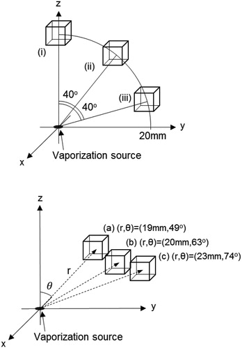
The ionization regions are represented by a cube with a 5 mm side length. Figure 3 shows the relative positions of the ionization regions. The boxes are arranged at three positions, (i), (ii), and (iii), and are located 20 mm from the origin of xyz coordinate system (Figure 3). The polar angles from the z-axis are 0$°,$ 40$°,$ and 80$°,$ respectively, for positions (i), (ii), and (iii). The ionizer boxes are also arranged at three positions, (a), (b), and (c), following the experimental setup given in Uchida et al. (2019). The number of A and B molecules inside the box is counted to estimate the ionization efficiency.

Figure 3. Positions of the ionization regions relative to the origin. The ionization region is represented by a cube with a 5 mm side length that is arranged at positions (i), (ii), (iii), (a), (b), and (c). Positions (i), (ii), and (iii) are located 20 mm from the origin and have polar angles of 0°, 40°, and 80°, respectively. Positions (a), (b), and (c) are arranged to fit the experimental condition in Uchida et al. (2019), and are located at 19, 20, and 23 mm from the origin, respectively, with polar angles of 49°, 63°, and 74°, respectively.

We ran the model either with or without molecular collisions to investigate the molecular collision effects. The model simulations needed to be validated by experimental data and/or independent analysis methods. The simulations without collisions can be compared with the analytical solution provided by Murphy (2016). We ran a specific simulation reported in Suwa and Fujii (2012) as a benchmark test for the simulations with collisions (see the SI).

The simulations were conducted using the Igor Pro version 6.37 software package and a personal computer (DELL OPTIPLEX 3020). The calculation time was about a day for each simulation run. The computer code used in our simulations is available in the SI.

3. Results

3.1. Simulations without molecular collisions

Figure 4 shows an example of temporal evolution of the number of molecules evaporating from an area source and staying in the ionization region at each position without molecular collisions. The NH₃ molecules generally had larger thermal velocities and reached the ionizer box earlier than the HI molecules. Both the NH₃ and HI molecules exhibited a similar temporal evolution among the three positions, suggesting that the spatial expansion of plumes was nearly isotropic, regardless of the molecular weight. The integrated ion signal for each species s, Q_s, was calculated using the time-integration of the number density of molecules in the ionizer and electron ionization cross-section for species s. Table 1 shows the ratio of the integrated signal for the NH₃ molecules to that for the HI molecules (Q_NH3/Q_HI). The electron ionization cross sections for NH₃ and HI at 60 eV were taken from the NIST database and Vinodkumar et al. (2010). The Q_NH3/Q_HI ratios were found to be nearly independent of the relative positions of the vaporization source and ionizer if the molecular collisions were not considered.

Figure 4. Temporal evolution of the number of molecules evaporating from the vaporization source and staying in the ionization region at positions (i), (ii), and (iii), without molecular collisions. The time step was set to 0.1 μs. The black and gray lines represent the number of NH₃ and HI molecules, respectively.

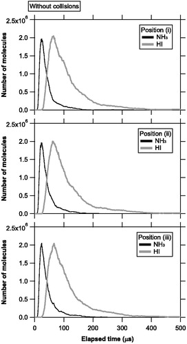
Table 1. Q_NH3/Q_HI ratios at each position for the base case simulations.^a

Position	Polar angle (°)	QNH3/QHI
		Without collisions	With collisions
(a)	49	0.168	0.197
(b)	63	0.173	0.229
(c)	74	0.173	0.270
(i)	0	0.172	0.151
(ii)	40	0.170	0.182
(iii)	80	0.172	0.294

^a The simulations were performed three times for each setting, and the values in this table represent the average of three simulation runs. The variation of these runs was less than 3%.

Murphy (2016) suggested that the residence time of the gas molecules in the ion source should be considered to estimate the sensitivity of a TDAMS, and incorporated the square root of the molecular weight ($\sqrt{MW}$) dependence in estimating the ionization efficiency. The ratio of $\sqrt{MW}$ for NH₃ to that for HI is ∼0.36. The ratio of the ionization cross section for NH₃ to that for HI is ∼0.47. Table 1 indicates that the Q_NH3/Q_HI ratios without collisions were in agreement with the product of the ionization cross-section and $\sqrt{MW}$ ratios (∼0.17), within the uncertainties, regardless of position. This result demonstrates that the numerical simulation without collisions is consistent with the analytical solution provided by Murphy (2016).

3.2. Simulations with molecular collisions

3.2.1. Spatial distributions

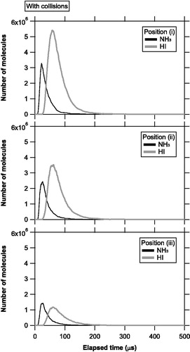
Figure 5 illustrates an example of the temporal evolution of the number of molecules evaporating from the source and staying in the ionization region at each position with molecular collisions. The temporal evolution curves for the HI molecules were generally narrower in the collision simulations (i.e., the molecular velocities were generally faster) compared to those in the collision-free simulations. Furthermore, the peak value of the temporal evolution curve for the HI molecules at position (iii) was ∼5 times smaller than that at position (i), in contrast to the twofold difference for the NH₃ molecules. Table 1 shows the simulated Q_NH3/Q_HI ratios.

Figure 5. Temporal evolution of the number of molecules evaporating from the vaporization source and staying in the ionization region at positions (i), (ii), and (iii), with molecular collisions. The black and gray lines represent the number of NH₃ and HI molecules, respectively.

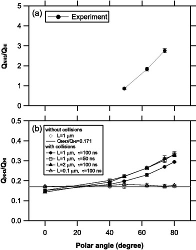
Figure 6 summarizes the measured and simulated Q_NH3/Q_HI ratios as a function of polar angle. The measured Q_NH3/Q_HI ratios for positions (a), (b), and (c) were 0.86 ± 0.04, 1.83 ± 0.09, and 2.76 ± 0.10, respectively (Uchida et al. 2019), whereas much smaller Q_NH3/Q_HI ratios were obtained from the simulations. There are a number of simplifications in the model, including the vaporization source profile and diagnostics of the probability of collisions. Nevertheless, our simulations show that the angular distribution of the NH₃ molecules is systematically different to that of the HI molecules when the molecular collisions are considered. This difference was more evident when the source area became larger or vaporization time scale was shortened, which was probably due to the increased gas molecules during the early stage of plume expansion. Conversely, the simulation with L = 0.1 μm suggests that molecular collisions may not be important for the vaporization of a single isolated particle. We interpret that the frequency of collisions were enhanced for the larger vaporization source areas due to increases in the molecular fluxes in the x and y directions. Although the potential importance of molecular collisions was pointed out by Drewnick et al. (2015) and Murphy (2016), this study is the first to quantitatively estimate this effect.

Figure 6. (a) Ratio of the integrated signal for the NH₃ molecules to that of the HI molecules (Q_NH3/Q_HI) obtained during the laboratory experiments. (b) The Q_NH3/Q_HI ratios obtained via the model simulations with and without molecular collisions. We assumed various values for the side length of the vaporization area, L, and vaporization time scale, τ. The solid circles represent the base-case simulations for (L, τ) = (1 μm, 100 ns).

3.2.2. Velocity distributions

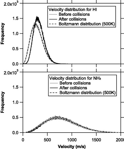
Figure 7 shows the velocity distributions of the NH₃ and HI molecules before and after the molecular collisions for the base case simulations. The velocity distributions of the NH₃ and HI molecules prior to collisions were in good agreement with the Boltzmann distribution at 500 K, as assumed. However, the velocity distribution of the HI molecules after the collisions exhibited a significant shift and was not well approximated by the Boltzmann distribution. This result suggests that (1) molecular collisions can alter the velocity distributions of the evolved gas molecules, and (2) the molecular velocities may not reach a thermal equilibrium within the simulation time. The total kinetic energy of the HI molecules after the collisions significantly increased (∼20%) as compared to that before the collisions, whereas the total kinetic energy of the NH₃ molecules just slightly increased (∼3%). Analysis of the energy budget shows that the molecules that intersect the hot surface (by reverse motions after collisions) tend to receive additional kinetic energies from the surface. We interpret that the kinetic energies were further transferred from the NH₃ molecules to the HI molecules during the molecular collisions. The molecular mean thermal velocities exhibit a $\sqrt{MW/T}$ dependence. The temperature effect may partially cancel out the molecular weight effect proposed by Murphy (2016) if heavier molecules tend to receive more kinetic energies than lighter molecules.

Figure 7. Velocity distributions of the NH₃ and HI molecules before (solid gray line) and after (solid black line) molecular collisions for the base case simulations. The Boltzmann distributions at 500 K are also shown as dashed black line.

4. Discussion

A common feature that is inferred from our laboratory experiments and simulations with collisions is that the NH₃ molecules were generally spread over broader regions than the HI molecules. However, we found significant discrepancies in the absolute values of the Q_NH3/Q_HI ratios between the experiments and simulations. One possible explanation is that the complexity of the source profiles in the experimental setup had a large effect on the angular distribution of gas molecules. Another possibility is that molecular translational velocities were affected by the inelastic collisions, which were dependent on the internal degrees of freedom of the molecules (translation, vibration, and rotation). NH₃ molecules would be more sensitive to this effect than HI molecules due to their molecular structures. It is important to note that these two potential mechanisms would not appear in the absence of molecular collisions. A direct measurement of the translational velocities of the NH₃ and HI molecules that evolved from NH₄I particles (or NH₃ and hydrogen chloride from ammonium chloride particles) may provide useful insights into the potential changes in the molecular velocities during the collisions.

While our simulation results are only applicable to limited model conditions, they have important implications for the vaporization process in the Aerodyne AMS. As Figure 1b shows, film boiling may occur when the particles are vaporized via impaction onto a heated surface. The number concentration of the gas molecules in a thin film layer may become much higher than that of the surrounding vacuum conditions, leading to a significant occurrence of molecular collisions, which can potentially affect the collection and ionization efficiency of aerosol particles. Molecular collisions may induce gas-phase reactions during the expansion of plumes. In fact, Drewnick et al. (2015) suggested the possible importance of gas-phase reactions during the early stage of plume expansion to explain the fragment patterns and vaporization time scale of ammonium nitrate particles detected by the Aerodyne AMS.

5. Conclusions

We investigated the dynamics of evolved gas molecules from aerosol particles in a TDAMS using a newly developed numerical model for simulating molecular collisions. Ensembles of NH₄I particles containing equal numbers of NH₃ and HI molecules were distributed, assuming a 1 μm × 1 μm source area and a 100 ns vaporization time scale. The simulations that incorporated molecular collisions demonstrated that the NH₃ molecules were generally spread over broader regions than the HI molecules. Although our simulations did not quantitatively explain the experimental results in Uchida et al. (2019), various processes induced by the molecular collisions may potentially fill the gap between the model and experimental results.

In summary, our study suggests that the molecular collisions during the early stage of plume expansion and possible changes in the molecular velocities induced by collisions could be an important mechanism affecting the observed variability in the ionization efficiency of TDAMSs. However, the physical and chemical processes of the vaporization and ionization of aerosol particles in TDAMSs may be too complex to be quantitatively reproduced using simplified numerical models. Despite the complexity, such theoretical studies provide an essential step toward obtaining a better understanding of the various types of aerosol particles detected by TDAMSs.

Additional information

Funding

This study was funded by the Grant-in-Aid for Scientific Research of the Japan Society for the Promotion of Science (JSPS) [16H05620 and 17H01862].

References

- Bird, G. A. 1994. Molecular gas dynamics and the direct simulation of gas flows. Oxford: Oxford University Press.
- Drewnick, F., J.-M. Diesch, P. Faber, and S. Borrmann. 2015. Aerosol mass spectrometry: Particle–vaporizer interactions and their consequences for the measurements. Atmos. Meas. Technol. 8 (9):3811–3830. doi: 10.5194/amt-8-3811-2015.
- Jayne, J. T., D. C. Leard, X. F. Zhang, P. Davidovits, K. A. Smith, C. E. Kolb, and D. R. Worsnop. 2000. Development of an aerosol mass spectrometer for size and composition analysis of submicron particles. Aerosol Sci. Technol. 33 (1–2):49–70. doi: 10.1080/027868200410840.
- Murphy, D. M. 2016. The effects of molecular weight and thermal decomposition on the sensitivity of a thermal desorption aerosol mass spectrometer. Aerosol Sci. Technol. 50 (2):118–125. doi: 10.1080/02786826.2015.1136403.
- Nanbu, K. 1980. Direct simulation scheme derived from the Boltzmann equation. I. Monocomponent gases. J. Phys. Soc. Jpn. 49 (5):2042–2049. doi: 10.1143/JPSJ.49.2042.
- Nanbu, K., Y. Watanabe, and S. Yonemura. 2000. Simulation method of flows in transitional and free-molecular regimes – Application to pumping of narrow gap between large plates. J. Vac. Soc. Jpn. (Shinku) 43 (10):2000. (in Japanese).
- Ng, N. L., S. C. Herndon, A. Trimborn, M. R. Canagaratna, P. L. Croteau, T. B. Onasch, D. Sueper, D. R. Worsnop, Q. Zhang, Y. L. Sun, and J. T. Jayne. 2011. An aerosol chemical speciation monitor (ACSM) for routine monitoring of the composition and mass concentrations of ambient aerosol. Aerosol Sci. Technol. 45 (7):780–794. doi: 10.1080/02786826.2011.560211.
- Saleh, R., E. S. Robinson, A. T. Ahern, and N. M. Donahue. 2017. Evaporation rate of particles in the vaporizer of the Aerodyne aerosol mass spectrometer. Aerosol Sci. Technol. 51 (4):501–508. doi: 10.1080/02786826.2016.127110.
- Seinfeld, J. H., and S. N. Pandis. 2006. Atmospheric chemistry and physics. 2nd ed. New York: John Wiley and Sons.
- Suwa, Y., and S. Fujii. 2012. Numerical simulation of rarefied gas mixture by DSMC method. Earozoru Kenkyu 27:292–305. (in Japanese).
- Takahama, S., and L. M. Russell. 2011. A molecular dynamics study of water mass accommodation on condensed phase water coated by fatty acid monolayers. J. Geophys. Res. 116:D02203. doi: 10.1029/2010JD014842.
- Takegawa, N., T. Miyakawa, T. Nakamura, Y. Sameshima, M. Takei, Y. Kondo, and N. Hirayama. 2012. Evaluation of a new particle trap in a laser desorption mass spectrometer for online measurement of aerosol composition. Aerosol Sci. Technol. 46 (4):428–443. doi: 10.1080/02786826.2011.635727.
- Uchida, K., Y. Ide, and N. Takegawa. 2019. Ionization efficiency of evolved gas molecules from aerosol particles in a thermal desorption aerosol mass spectrometer: Laboratory experiments. Aerosol Sci. Technol. 53 (1):86–93. doi: 10.1080/02786826.2018.1544704.
- Vinodkumar, M., R. Dave, H. Bhutadia, and B. K. Antony. 2010. Electron impact total ionization cross sections for halogens and their hydrides. Int. J. Mass Spectrom. 292 (1–3):7–13. doi: 10.1016/j.ijms.2010.02.009.
- Yasuhara, M., and H. Daiguji. 1992. Computational fluid dynamics – Fundamental and application. Tokyo: Tokyo Daigaku Shuppan Kai. (in Japanese).
- Zhang, Q., et al. 2007. Ubiquity and dominance of oxygenated species in organic aerosols in anthropogenically influenced northern hemisphere midlatitudes. Geophys. Res. Lett. 34:L13801. doi: 10.1029/2007GL029979.