
 ?Mathematical formulae have been encoded as MathML and are displayed in this HTML version using MathJax in order to improve their display. Uncheck the box to turn MathJax off. This feature requires Javascript. Click on a formula to zoom.
Abstract
Determination of the particle charge in aerosols and dusty plasmas requires an accurate calculation of the particle-ion collision kernel taking into account the particle-ion Coulombic coupling and ion-neutral gas molecule collisions. While the effect of Coulombic interactions of any strength is described accurately in the continuum limit and free molecular limit, an accurate physical description at intermediate collisional regimes remains elusive. Specifically, the Coulomb influenced collisions between oppositely charged particles and ions have evaded accurate theoretical description in the past. We use Langevin dynamics (LD) calculations to infer the non-dimensional collision kernel as a function of the electrostatic potential energy to thermal energy ratio
and the diffusive Knudsen number
the index of ion-neutral collisionality in a finite pressure system. The LD approach yields a simple, approximate treatment of particle charging in the entire ion-neutral collision regime under the assumption that
where
is the mass of an ion and
is the mass of the background gas molecules. We show that the Gumbel distribution accurately describes the underlying distribution of
calculated using LD. The effect of high ion concentrations (at which screening of particle by free charges in space is important) on
is parameterized through a non-dimensional screening length parameter
Analysis of the dependence of the distribution parameters on
and
leads to a regression for
that is valid for
and
plasmas. Inter-comparison of current model with select models from the literature shows that the current model and the model published by Gatti and Kortshagen (that assumes
) yield similar predictions for a wide range of
and
Copyright © 2019 American Association for Aerosol Research
Editor:
Introduction
The electric charge of micro- and nanoparticles determines their long-range electrostatic interaction, electrical mobility, growth kinetics and collective behavior in aerosols and dusty plasmas. Determination of the particle charge distribution is necessary for the inversion of measured electrical mobility distribution to obtain particle size distribution (Hagen and Alofs Citation1983; Hogan et al. Citation2009) and for the description of size-resolved growth dynamics in aerosols (Gelbard, Tambour, and Seinfeld Citation1980; In Jeong and Choi Citation2001; McMurry Citation2000; Wu and Flagan Citation1988). In dusty plasmas characterized by highly charged particles suspended in a partially ionized gas, self-assembly of particles (or grains) over mesoscopic length scales has been observed in controlled experiments (Molotkov et al. Citation2015; Nefedov et al. Citation2003; Pustylnik et al. Citation2016) and natural contexts (interplanetary nebulae, planetary rings). These “Coulombic crystals” are formed due to long- and short-range interactions between particles, primarily determined by their electric charge and plasma conditions (ion, electron concentrations, and electric fields). In both aerosol and plasma science, determination of the electric charge on particles plays a pivotal role in the theoretical description of the spatial and temporal dynamics of particulate populations.
The particle charge in gas-phase systems (aerosols/dusty plasmas) can vary by a variety of mechanisms—ion and electron fluxes collected by the particles via collisions and charge transfer (Khrapak and Morfill Citation2009), photoionization (Han et al. Citation2003; Jiang et al. Citation2007; Yun et al. Citation2009), thermionic emission (Autricque et al. Citation2018) and photoelectron emission by UV radiation, chemical ionization and so on (Fortov et al. Citation2005). In this article, we focus on particle charging by collisions with ions driven by the combined electrostatic motion and Brownian diffusion in the gas phase and in the absence of external electric fields. In typical aerosol systems, ions of both polarities have similar masses (∼50–600 amu) and electrical mobilities (). The particle charge varies nominally between ±20 in the sub-1 µm size range at atmospheric pressure (Gopalakrishnan, McMurry, and Hogan Citation2015; Gopalakrishnan, Meredith, et al. Citation2013; Wiedensohler Citation1988). Contrastingly, in non-thermal dusty plasmas, electrons are hotter than the positive ions (
) while the ions are equilibrated via collisions with neutral gas molecules (
) at a common temperature (Lieberman and Lichtenberg Citation2005). Further, electrons are also ∼10,000 times lighter than the ions that are typically derived from the ionization of the background gas molecules (
Thus, initially uncharged particles receive a higher electron current than ion current from the bulk plasma and rapidly attain a negative charge. The extent of the negative particle charge
on the particle roughly scales with the electron temperature and particle size (
). When the particle is sufficiently negatively charged, slow moving electrons are repelled causing a reduction in the electron current and thereby the ion flux eventually catches up with the electron flux leading to a stationary state charge on the particles. As a result, 0.1–10 µm particles carry
units of negative charges in typical low pressure, non-thermal dusty plasmas, making the collisions between highly negatively charged particles and positive ions the dominant charge transfer process. In both types of particulate systems, the collisions between unlike charged entities (particle and ion) in a background gas are dominated by attractive Coulomb interactions and Brownian diffusion. We restrict our scope to the collisions between particles and ions at thermal equilibrium with the gas. Collisions between particles and non-equilibrium ions/electrons are beyond our scope here.
By virtue of their high negative charge level (), grains/particles in a dusty plasma hold a finite number of positively charged ions in metastable orbits around them. These ions effectively shield the grain of its charge and the extent of screening is dependent on the ion concentration. While this effect is negligible at low ion concentrations (typical of atmospheric aerosols or low-strength bipolar neutralizers), high ion concentrations are routinely found in dusty plasmas, unipolar aerosol chargers, flames/plasmas generated for material synthesis, and cosmic environments (planetary nebulae, ionosphere, etc.). The charging of particles in high ion concentration environments where electrostatic screening of the particle is appreciable has been routinely considered by dusty plasma modelers (Khrapak and Morfill Citation2009). The screening of grains/particles by free charges in the gas phase leads to a non-trivial electrostatic potential around the particle that can be self-consistently calculated by simultaneously solving the ion and electronic concentration profile and the Poisson equation for the electrostatic potential (Bystrenko and Zagorodny Citation1999; Daugherty, Porteous, and Graves Citation1993; Khrapak and Morfill Citation2009). As an approximation, at low particle concentrations, the electrostatic potential around an isolated particle is often modeled using a Debye–Huckel potential that retards the classic
Coulomb potential exponentially with an effective Debye length
(Gatti and Kortshagen Citation2008; Lampe et al. Citation2003; Zobnin et al. Citation2008). The Debye screening length
is obtained from the linearization of the Poisson–Boltzmann equation to describe ion concentration and the electrostatic potential around the particle (Lieberman and Lichtenberg Citation2005). A screened Coulomb potential with a distance-dependent screening length has been recently shown to be a reasonable approximation for the electrostatic potential around a particle with strong particle-ion coupling (Semenov, Khrapak, and Thomas Citation2015). The continuous ion absorption and electron emission from the particle surface and ion flux conservation give rise to long range power-law asymptotes for the electrostatic potential around the particle. A bi-directional coupling between the particle surface electric potential (charge) and the ion and electron concentration near the particle using coupled Poisson–Boltzmann equation and species concentration equation has been used to infer the electrostatic potential (Daugherty et al. Citation1992; Fortov et al. Citation2005; Hutchinson and Patacchini Citation2007; Khrapak and Morfill Citation2009; Semenov, Khrapak, and Thomas Citation2015). The complex electrostatic potential deviates from a simple Coulomb form, especially at large particle-ion separations. However, in close proximities, although not entirely accurate, the modeling of the particle-ion electrostatic potential via a prescribed screened Coulomb potential allows physical insight into the effect of charge screening at high ion concentrations without much computational cost associated with simultaneously solving for the spatial ion concentration and the electrostatic potential around a particle. A complete analysis of particle charging taking into account the temporally changing, self-consistent electric potential and non-linear charge fluxes to the particle surface would require numerical calculations using diffusion-based approaches (Tarasov and Veshchunov Citation2018) or particle-in-cell (PIC) methods (Hutchinson and Patacchini Citation2007). In aerosol science, by virtue of relatively dilute ion concentrations and low charge levels (
units of charge), the charging of particles at high ion concentrations has been scarcely investigated experimentally (Adachi et al. Citation1989; Pui, Fruin, and McMurry Citation1988). The focus has largely been on the effect of image potential on the attachment of small ions onto aerosol particles due to electrostatic attraction. In addition to the thermal energy and electrostatic energy of the ion, charge screening due to excess space charge (ion) concentration also determines the particle charge distribution by reducing the effective charge on the particles and needs to be described accurately. In this article, we focus on electrostatic interactions between particle and ion due to a simple Coulomb potential in the presence of background gas molecules. Further theoretical development to include image potential interactions and other short-range interactions may be built upon using the approach and results described in this article.
The charging rate of particles of a certain size per unit volume per unit time is calculated as the product of the particle concentration
ion concentration
and the particle-ion collision kernel
that describes the particle-ion interaction:
The unperturbed (positive/negative) ion concentration
and particle concentration
is obtained from Langmuir probe measurements (Hopkins and Graham Citation1986; Merlino Citation2007) or optical diagnostics (Melzer et al. Citation2018) in a dusty plasma (Bonitz, Henning, and Block Citation2010; Chaudhuri et al. Citation2011; Mann et al. Citation2011; Molotkov et al. Citation2015; Shukla and Eliasson Citation2009). In aerosol systems, condensation particle counters (CPCs) allow the direct measurement of particle concentration (Stolzenburg and McMurry Citation1991) and the ion concentration is obtained via electrometer measurements. Tandem ion mobility spectrometry-mass spectrometry (IMS-MS) techniques have been employed to obtain the mass-mobility distribution of charging ions as well (Gopalakrishnan, McMurry, and Hogan Citation2015; Maißer et al. Citation2015). The collision kernel
encompasses the collision physics and is calculated from a suitable model of particle-ion collision in the presence of a background gas. Development of models for
has been the subject of many prior investigations in the field of aerosol science and dusty plasmas. We begin by reviewing important theoretical developments with appropriate context to the respective field.
The orbital motion limited (OML) theory (Allen Citation1992; Mott-Smith and Langmuir Citation1926), based on the conservation of energy and angular momentum of an ion colliding with a particle, is widely used in the field of dusty plasmas to calculate the collision kernel Ion-neutral collisions destroy conservation of these quantities and make OML inapplicable for particle charging in moderate and high-pressure dusty plasmas.
(
) is referred to as ion flux coefficient in the plasma literature and defined as the ratio of the ion current
(
) collected by the particle to the ion concentration
multiplied by the charge on an electron (
) (Khrapak and Morfill Citation2009; Morfill and Ivlev Citation2009; Shukla and Eliasson Citation2009). By construction, OML assumes transport of the charges to the particles without considering collisions with neutral background gas molecules via purely ballistic motion making it strictly applicable only in perfect vacuum (gas pressure → 0). The ions are assumed to have a Maxwell–Boltzmann distributed velocity in their approach towards the particle (Allen Citation1992). The application of OML theory to the calculation of (positive) ion currents collected by (negatively charged) particles in dusty plasmas leads to significant differences between the predicted and measured charge on the particles at pressures ∼10–1000 Pa. The most significant assumption of the OML theory that is not met in moderate pressure dusty plasmas is the neglect of ion-neutral gas molecule collisions. Ion trajectories around a particle are distorted by collisions with neutral gas molecules (Goree Citation1992). The neutrals scatter momentum and energy that destroys deterministic ion orbits and lead to a higher ion current than predicted by OML. This effect has been observed in many computational investigations (Gopalakrishnan and Hogan Citation2012; Hutchinson and Patacchini Citation2007; Vaulina, Repin, and Petrov Citation2006; Zobnin et al. Citation2000) and it is expected that the particle charge would be less negative than if the ion current were calculated using collision-less OML. The mean charge on the particles is seen to be about 2–4 times lower than the value predicted by OML. Fortov et al. (Citation2004) report that the mean charge on 1.8 and 12.7 µm particles is nearly 4 times smaller than the predictions of OML in a RF neon discharge of frequency 100 MHz operated between 20 and 50 Pa. Ratynskaia et al. (Citation2004) investigated the charging of 0.6 µm particles between 20 and 100 Pa and found that the charge is systematically lower than the OML prediction. They attribute the reduction in particle charge to ion-neutral collisions that increase ion collection by the particles. Khrapak et al. extended the pressure range to 150 Pa and remark that their measurements are systematically lower than OML predictions (Khrapak et al. Citation2005, Citation2012), reaffirming the over-prediction of particle charge (or under-prediction of the ion flux coefficient).
Analytic modeling has been undertaken to account for the ion-neutral gas molecule collisions in particle charging. The idea of dividing the space around a charged particle into two zones, a highly collisional outer zone in which ion transport can be described via a Fokker–Planck type diffusion equation and an inner zone of very low collisionality close to the particle wherein a vacuum picture can be applied, has led to several avatars of the flux matching model (Bricard Citation1962; D’Yachkov et al. Citation2007; Fuchs Citation1963; Hoppel and Frick Citation1986; Lopez-Yglesias and Flagan Citation2013; Lushnikov and Kulmala Citation2004; Marlow Citation1980). The continuum and ballistic fluxes are matched at the surface of a limiting sphere to idealize the transition from continuum transport of ions to a rarefied motion near the particle. This idealization of the ion motion to purely ballistic motion is in practice realized when the ion is much lighter compared to the background gas molecules, thereby making the model exact in the limit of the ratio comparing mass of the ion
to mass of the background gas molecules
approaching zero, i.e.,
However, the increase in kinetic energy of the ion as it arrives at the surface of the limiting sphere, and within the limiting sphere due to the particle-ion attractive potential is not accounted for in this model (Filippov Citation1993; Gopalakrishnan and Hogan Citation2012; Gopalakrishnan, Thajudeen, et al. Citation2013; Ouyang, Gopalakrishnan, and Hogan Citation2012). Further, when the motion of the ion inside the limiting sphere was assumed collision-less, a first order correction was necessary to account for ion-neutral collisions (also referred to as resonant charge exchange collisions in the dusty plasma literature and three-body trapping in the aerosol science literature) and later it was recognized that higher order corrections may be necessary as well (Hoppel and Frick Citation1986). This model requires the estimation of the probability of ion capture by the particle while moving inside the limiting sphere making it dependent on free parameters such as the radius of the limiting sphere and the capture probability. In the field of aerosol science, the flux matching model by Fuchs (Citation1963) has been tested against measured charge fractions (Adachi, Kousaka, and Okuyama Citation1985; Hussin et al. Citation1983; Porstendörfer et al. Citation1984; Reischl, Scheibel, and Porstendörfer Citation1983; Wiedensohler et al. Citation1986) and often free parameters in the model are chosen to force agreement with predictions (Reischl et al. Citation1996; Stober, Schleicher, and Burtscher Citation1991; Wiedensohler and Fissan Citation1988), thereby clouding the validity of the theory itself (Gopalakrishnan, McMurry, and Hogan Citation2015; Liu and Pui Citation1974).
Gatti and Kortshagen (Citation2008) recognized that in order to scatter enough momentum for an ion to be eventually trapped by the particle, a very small number of collisions with neutrals is sufficient. Based on this idea, they proposed that the ion current can be calculated by accounting for just three types of transport: collision-less capture of ions that is described by the classical OML result (Allen Citation1992), the continuum or infinitely collisional limit (Fuchs Citation1964) and as an intermediate case—the capture of ions due to exactly one collision with a neutral in its approach towards the particle. Similar to the flux matching model, Gatti and Kortshagen’s model also implicitly assumes that the ion is much lighter than the background gas molecules, i.e., They calculated the ion current as the sum of the current due to each of the three transport mechanisms weighted by their respective probabilities (Varney Citation1971) based on the ion mean free path relative to a “capture radius”
and obtained excellent agreement with dusty plasma charging experiments cited before. They advanced the notion that the capture radius
calculated as the radial distance at which the ion’s mean kinetic energy
equals to the electrostatic potential energy
is the appropriate length scale for describing the particle-ion interaction (Lushnikov and Kulmala Citation2004):
At moderate gas pressures, an ion’s motion could still be influenced by multiple collisions with neutrals and an accurate book keeping of ion-neutral collisions is necessary to capture the enhancement in the ion current accurately.
Semi-empirical expressions have been proposed to fit the results of ab initio molecular dynamics (MD), PIC, and Langevin dynamics (LD) calculations of particle-ion collisions in the presence of background gas molecules (Gopalakrishnan and Hogan Citation2012; Hutchinson and Patacchini Citation2007; Iza and Lee Citation2006; Lampe et al. Citation2003; Lampe and Joyce Citation2015; Taccogna, Longo, and Capitelli Citation2003; Trunec et al. Citation2004; Vaulina, Repin, and Petrov Citation2006; Zobnin et al. Citation2000). Hutchinson and Patacchini (Citation2007) derived an empirical fit to the ion current obtained from PIC calculations for a wide range of gas pressures or ion-neutral collisionalities including interactions between ions and electrons. They show good agreement with the calculations by Lampe et al. (Citation2003) in which the presence of neutrals is accounted for by solving ion-neutral collision integrals. Zobnin et al. (Citation2008) solved the Boltzmann equation with a constant ion-neutral collision frequency and developed a fit to their results across a wide range of collisionalities. Their fit also converges to the OML limit as collision frequency → 0 and to the current calculated by continuum models (Yaroshenko et al. Citation2004) that take into account ion drift and diffusion at high gas pressures (i.e., strongly collisional plasma). It must be noted that approaches based on solutions to various approximations of the Boltzmann equation implicitly or explicitly assume that the ions are much lighter than the background gas
Vaulina, Repin, and Petrov (Citation2006) pioneered the application of LD, that implicitly accounts for ion-neutral collisions via the drag force on the ion due to neutrals and the rapidly fluctuating impulses in ion velocity and position due to Brownian diffusion in addition to electrostatic interactions, to compute the steady state charge on a non-emitting grain immersed in a non-thermal dusty plasma. They probed the effect of electron temperature, grain size and charge concentration and produced a simple parameterization for the mean charge (average potential) of the particle. They showed that LD greatly simplifies the determination of particle charge and ion current received by the particle for a wide range of ion-neutral collisionalities. The expression for the ion current put forward by Vaulina, Repin, and Petrov (Citation2006) from theoretical considerations was tested against the predictions of LD calculations of the mean charge on a non-emitting dust grain immersed in a non-thermal dusty plasma. Contrastingly, by analyzing LD calculations of the particle-ion collision time in the dilute limit (), Gopalakrishnan and Hogan (Citation2012) have proposed a model for the particle-ion collision kernel
The inverse of the non-dimensional particle-ion collision time in a periodic domain was interpreted as a non-dimensional collision kernel
(which is elaborated upon shortly and referred to as
). Both Vaulina, Repin, and Petrov (Citation2006) and Gopalakrishnan and Hogan (Citation2012) have used LD to infer
by considering particle-ion collisions. The simulations of Vaulina, Repin, and Petrov (Citation2006) allowed the particle charge to equilibrate in the presence of positive ion and electron collisions without considering ion-ion, ion-electron or electron-electron interactions. Gopalakrishnan and Hogan (Citation2012) took a similar approach in which only particle-ion interactions were considered along with the effect of neutrals using the Langevin equation. As will be discussed later, these models yield similar predictions for a wide range of particle-ion collision parameters. The Langevin-inferred
is accurate in the limit of the ratio
comparing mass of the ion
to mass of the background gas molecules
approaching infinity, i.e.,
The LD approach provides an approximate treatment for the collision kernel in the entire transition regime and has been applied to derive an expression for the collision kernel that describes coagulation (Gopalakrishnan and Hogan Citation2011; Thajudeen, Gopalakrishnan, and Hogan Citation2012), vapor condensation (Gopalakrishnan, Thajudeen, and Hogan Citation2011; Ouyang, Gopalakrishnan, and Hogan Citation2012), and unipolar charging (Gopalakrishnan, Thajudeen, et al. Citation2013) of arbitrarily shaped particles. Gopalakrishnan and Hogan (Citation2012) laid out a phase space diagram of ion-neutral gas molecule collisionality (parameterized by a diffusive Knudsen number
) and particle-ion electrostatic energy (parameterized by an electrostatic potential to thermal energy ratio of the ion
for attractive Coulombic interactions).
is defined as the ratio of the average distance traveled by the ion before it completely changes direction, i.e., the mean persistence distance of the ion motion relative to the particle size. At high pressures, the particle-ion motion is dominated by Brownian diffusion and results in small persistence distances (
At low pressures, the ion motion is nearly ballistic and is dominated by inertial effects (
by definition, is an index of the collisionality or collision frequency between ions and neutral gas molecules and is used to parameterize the effect of ion-neutral collisions on the ion transport onto the surface of the particle (and lead to particle charging). We note that, in the plasma literature the ion collisionality index is usually defined as the ratio of the ion mean free path to the plasma screening length. Our definition of
parameterizes the ion-neutral collisionality in comparison to the particle size as a length scale. Likewise, particle-ion interactions dominated by thermal energy or absence of any electrostatic interaction corresponds to low
while interaction between highly charged particles and ions lead to high values of
Gopalakrishnan and Hogan (Citation2012) developed models for the non-dimensional collision kernel
for the cases of hard spheres interactions (
and all
), high potential near continuum regime (large
and small
) and repulsive interactions (
and all
). The high potential, near free molecular regime (large
and large
), was not parameterized in their model development as they were not able to derive a model that converged to the correct free molecular (or OML limit) as ion-neutral collisionality approaches zero (or
The charging of sub-20 nm particles at atmospheric pressure, charging of ∼1 µm particles in a ∼100 Pa dusty plasma are a few instances wherein the collision between particles and ion leads to a
> 100 and
In this article, we develop a model for
for a wide range of ion-neutral collisionalities and particle-ion coupling strengths, especially those corresponding to the high potential, near free-molecular charging regime. In contrast with prior work on the use of LD to develop collision kernel expressions, our approach here consists of parameterizing the underlying distribution of particle-ion collision times inferred from LD. A description of the underlying distribution and its dependence on
allows the calculation of
as a function of properties of the colliding particle and ion. We develop approximate, easy-to-use expressions for the flux coefficient
for both Coulomb and screened Coulomb (also known as retarded Coulomb or Debye–Huckel) potentials for
and
Computational methods
Theoretical analysis of Coulombic particle-ion collisions
We consider a spherical particle of radius charge
and a point ion of mass
charge
and friction factor
(related to the low-field ion mobility
and diffusion coefficient
=
) in the presence of neutral gas molecules that are in thermal equilibrium with the ions at a common temperature
The particle and ion interact through the classical Coulomb potential
and in dilute conditions (Debye length
). By choosing the particle radius
as the length scale of the particle-ion Coulomb coupling, the relative importance of the particle-ion electrostatic potential energy to the ion’s thermal energy is parameterized by
In the continuum or infinitely collisional limit of ion motion, continuum modeling has been employed to derive
in the presence of Brownian diffusion and electrostatic drift of point-like ions towards a large, spherical particle. In this regime,
is given by the classic Smoluchowski equation that depends on the ion friction factor
particle radius
and an enhancement factor
(1a)
(1a)
The enhancement factor can be evaluated using the Fuchs integral (Friedlander Citation2000; Fuchs Citation1963) for the Coulomb potential
as:
(1b)
(1b)
In the collision-less or free molecular limit, methods of kinetic theory of gases have been applied to derive a model for assuming that the ions start far away from the particle with a Maxwell–Boltzmann distributed velocity and do not suffer any collisions with neutrals until they are collected by the particle.
is dependent on the mean thermal speed of the ion and the effective free molecular particle-ion collision cross section. Analogous to the continuum enhancement factor, a free molecular enhancement factor
is used to account for the electrostatic potential:
(2a)
(2a)
By considering the conservation of angular momentum and kinetic energy of the ions, an expression for the free molecular enhancement factor is derived as (Allen Citation1992; Mott-Smith and Langmuir Citation1926):
(2b)
(2b)
The LD calculation of 
Equations (1) and (2) describe the continuum (infinitely collisional) and free molecular (collision-less) limits of respectively and offer an important physical insight. The continuum limit depends only on the ion’s diffusivity (or friction factor
) while the free molecular limit depends only on the ion’s inertia (mass
), while both limits depend on the particle size
gas temperature
and the particle-ion electrostatic energy ratio
At intermediate pressures or collisionalities,
depends only on the parameters that affect it in continuum and free molecular limits. In such instances, the ion motion is neither entirely diffusive nor ballistic to be accurately described by continuum or kinetic approaches (Gopalakrishnan and Hogan Citation2012). For such circumstances, a Langevin description of ion motion has been successfully employed in the past to derive approximate collision rate coefficients or kernels, and to predict the dilute transport of species in a background gas (Gopalakrishnan and Hogan Citation2011; Narsimhan and Ruckenstein Citation1985). The Langevin treatment is strictly applicable only in instances wherein the ratio of the mass of the ion
to the mass of the background gas molecules
approaches infinity, i.e.,
(Mazur and Oppenheim Citation1970). In practice,
for ions found in typical aerosol charging environments with typical mass of positive ions ∼100 g/mole and negative ions ∼50 g/mole (Adachi, Kousaka, and Okuyama Citation1985; Gopalakrishnan, McMurry, and Hogan Citation2015; Maißer et al. Citation2015) in air or nitrogen. In non-thermal dusty plasmas,
for
or simple ions formed by the direct ionization of the discharge gas. In the continuum regime, it is known that continuum based approaches (
) and approximations to the Boltzmann equation (that assume
yield identical expressions for the collision kernel (Veshchunov Citation2010, Citation2011; Veshchunov Citation2012; Veshchunov and Azarov Citation2012). The influence of
on the electrostatically influenced diffusion of ions to the particle surface in the transition and free molecular transport regimes remain hitherto unexplored. However, the effect of
and ion-neutral collisions can be indirectly inferred by comparing the predictions of transition regime collision kernel expressions derived under drastically different assumptions of
and computational approaches. Gopalakrishnan and Hogan (Citation2011) compared, for hard sphere interactions between two spheres and a sphere and a point mass, the predictions of several collision kernel expressions that assume
or
in their construction. LD (Gopalakrishnan and Hogan Citation2011), diffusion theory (Veshchunov Citation2010) and other approaches (Dahneke Citation1983; Fuchs Citation1964) that assume
yield predictions that are neither systematically different nor differ more than
from the predictions of the models derived by solving the Boltzmann equation to model vapor transport to an absorbing particle with
(Fuchs and Sutugin Citation1970; Loyalka Citation1982). Although this comparison was made for hard sphere interactions, it is instructive that the influence of
on the collision kernel is presumably no larger than the statistical variation associated with LD computations. Clearly, further work is necessary to clarify the role of
further and that if the collision kernel is a stronger function of
as
and in the presence of potential interactions. The charging of particles by ions in non-thermal dusty plasmas are typically due to ions that are of the same mass of the background gas molecules (for example,
in
leading to
). In aerosol systems, heavier bipolar charging ions lead to
The charging by electron collisions or ions lighter than the background gas, for which
is beyond the scope of the modeling here. Due to the lack of a significant difference between the predictions of collision kernels that assume
and
in prior work, we use the Langevin equation to describe the particle-ion collision in the frame of reference of the particle to describe particle charging in the
limit. A rigorous treatment of ion transport onto the surface of a charge particle suspended in a background gas should be treated via the Boltzmann equation. This fact notwithstanding, the Langevin description applied here is later justified by qualitative and reasonable quantitative agreement between Langevin-inferred
(assuming
) and the predictions of models that assume
in a posteriori comparison:
(3)
(3)
Here, is the relative velocity of the ion with respect to the particle,
is the sum of all external forces on the ion and
is a fluctuating impulse force term used to model the thermal diffusion of the ion (Chandrasekhar Citation1943). To scale the equations and express them in physically significant units, length is expressed in multiples of the particle radius
time in terms of the ion relaxation time
and
is identified as a reference velocity. By non-dimensionalizing the solution to EquationEquation (3)
(3)
(3) originally derived by Ermak and Buckholz (Citation1980), we track the ions in the space around the particle using an explicit equation for its non-dimensional velocity
and position
(4a)
(4a)
(4b)
(4b)
(4c)
(4c)
(4d)
(4d)
and
are normally distributed random displacement and velocity vectors that are added to the solution at each time step to capture the effect of Brownian fluctuations (Ermak and Buckholz Citation1980).
and
have a mean of zero and variances given by EquationEquations (4b)
(4b)
(4b) and Equation(4d)
(4d)
(4d) . Ermak and Buckholz (Citation1980) solved EquationEquation (3)
(3)
(3) as a stochastic differential equation with vectors
and
added to the deterministic part of the solution to capture the thermal fluctuations in the velocity and position, respectively, due to ion-neutral gas molecule collisions.
is the non-dimensional force acting on the ion and is an explicit function of the ion position
For the case of unscreened Coulomb interaction between the particle and ion,
and
are given by EquationEquations (1b)
(1b)
(1b) , Equation(2b)
(2b)
(2b) respectively. From the non-dimensionalization, we recognize that the ion’s motion depends on two dimensionless numbers—the potential energy ratio
and the diffusive Knudsen number
an index of ion-neutral collisionality:
(5)
(5)
The expression for the diffusive Knudsen number well established as a parameter in diffusion-limited mass transfer (Dahneke Citation1983; Loyalka Citation1976; Rogak and Flagan Citation1992), is a ratio of the mean ion persistence distance
and an effective length scale characterizing the particle-ion electrostatic interaction
In the continuum (infinitely collisional) limit, the mean persistence path is much smaller than the length scale of the particle-ion interaction, i.e.,
Likewise,
denotes the free molecular (collision-less) limit of ion motion. Finally, we non-dimensionalize
to derive
Normalizing EquationEquations (1a)
(1a)
(1a) and Equation(2a)
(2a)
(2a) yield the continuum and free-molecular limits for
in
space:
(6a)
(6a)
(6b)
(6b)
At intermediate collisionalities, the non-dimensional collision kernel is a function of both
and
and should converge to the limits given by Equation (6) at the respective limits of
To infer
we employ the rate constant calculation procedure developed by Hogan and coworkers (Gopalakrishnan and Hogan Citation2011; Gopalakrishnan and Hogan Citation2012; Gopalakrishnan, Thajudeen, and Hogan Citation2011; Ouyang, Gopalakrishnan, and Hogan Citation2012; Thajudeen, Gopalakrishnan, and Hogan Citation2012). Briefly, the ion is initialized on the surface of a sufficiently large periodic box (
) with a velocity sampled from the Maxwell–Boltzmann distribution and tracked using Equation (4) until it collides with the particle
at the origin to obtain the collision time. The inverse of the mean binary particle-ion collision time
normalized by the simulation box volume
is interpreted as
based on statistically significant number (2000 here) of trials of the particle-ion collision:
(7)
(7)
The time step is chosen by the empirical condition that compares the diffusional and electrostatic force to determine the optimum timestep for computational efficiency:
The effect of the parameter 0.005 was empirically tested and chosen to balance computational accuracy and expense. The domain size was chosen as large as necessary to ensure that the ion started in conditions where its electrostatic potential energy is approximately zero. The following condition was used to determine
for each
model development for Coulombic collisions
For (hard-sphere interactions), prior work (Gopalakrishnan and Hogan Citation2011) has shown that
has the following functional form valid for all
and converges to the limits of EquationEquations (6a)
(6a)
(6a) and Equation(6b)
(6b)
(6b) :
(8)
(8)
EquationEquation (8)(8)
(8) also describes
including the effect of short-range, singular contact potentials (Ouyang, Gopalakrishnan, and Hogan Citation2012), and repulsive Coulombic
potential (Gopalakrishnan and Hogan Citation2012; Gopalakrishnan, Thajudeen, et al. Citation2013) when the appropriate enhancement factors
and
are calculated for the respective potentials and used in the definition of
and
For each
and
2000 independent trials of the particle-ion collision were simulated to build a histogram for
Here,
is calculated based on the particle-ion collision time for an individual trial (1
is the logarithm of the enhancement in
at a given
due to
compared to the corresponding hard sphere value
predicted by EquationEquation (8)
(8)
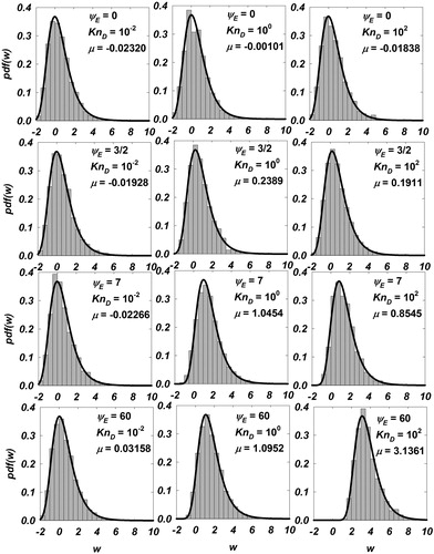
(8) . shows the normalized frequency histogram of
for
at high
), intermediate (
and low (
collisionalities. It is seen that the distributions are translated along the abscissa as
and
are varied, with their shape and magnitude intact. A Gumbel distribution (Coles Citation2001) with one location parameter
is found to describe the probability density function
with high statistical confidence (regression details in Section S1 of the online supplementary information [SI]):
(9)
(9)
Figure 1. Histograms of inferred from Langevin simulations are shown for
for
The gray bars represent the normalized counts
of
and the solid black line is the Gumbel distribution function (EquationEquation (9)
(9)
(9) ) with the corresponding value of location parameter
fitted for each case.
The Langevin simulation is a means to sample from an ensemble of infinite trajectories. The periodic domain restricts the sampling of
’s that represent the minimums from a possible infinite sequence of ion trajectories that also includes those in which the ion spends a long time away from the particle but are eliminated in the computer experiments. According to the Fisher–Tippett–Gnedenko theorem (Gnedenko Citation1948), these
values, the minimums of infinite sequences of
follow the Gumbel distribution which is a special case of the generalized extreme value distribution (Coles Citation2001). Using
of EquationEquation (9)
(9)
(9) ,
can be computed through the mean value of
(10)
(10)
To use EquationEquation (10)(10)
(10) for a given combination of
and
we fit
as a functional form. shows
for
and
A function with four fit constants
accurately fits the data:
(11)
(11)
Figure 2. Fitted values of the location parameter for
for
shown as data points. The corresponding fit for
(EquationEquation (11)
(11)
(11) ) is shown as dashed lines of the same color.
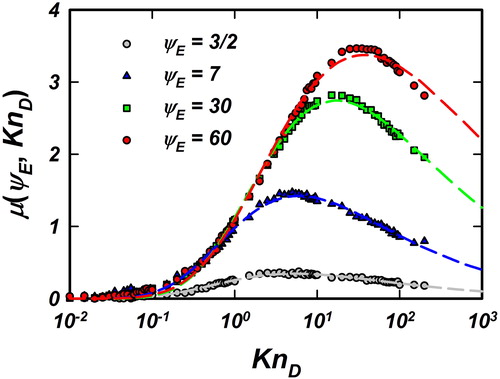
EquationEquation (11)(11)
(11) captures the dependence of
for
and approaches 0 as
and
ensuring that
converges to the limits of Equation (6). Regression fit for
are described in Section S2, SI. Thus, EquationEquation (10)
(10)
(10) can be used with EquationEquation (11)
(11)
(11) to predict
for
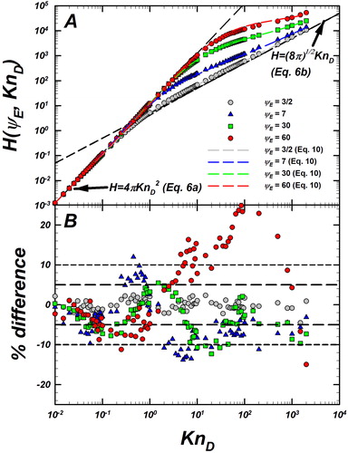
In , calculated using the mean collision time for 2000 collisions (EquationEquation (7)
(7)
(7) ) for
are plotted as a function of
Also shown on the plots are the continuum limit (EquationEquation (6a)
(6a)
(6a) ) and free-molecular limit (EquationEquation (6b)
(6b)
(6b) ). The model developed in this article (EquationEquation (10)
(10)
(10) with appropriate value of
) is presented to show the comparison with the Langevin-inferred
Using EquationEquation (11)
(11)
(11) in Equation(10)
(10)
(10) , dashed curves corresponding to each
were generated and compared against the Langevin-inferred
(EquationEquation (7)
(7)
(7) ) to calculate the % difference as
This comparison is plotted in for each case of
Immediately evident is that the model describes the Langevin-inferred
to within
accuracy for most data points, with few data points within
More importantly, the model of EquationEquation (10)
(10)
(10) is designed to approach the free molecular limit (EquationEquation (6b)
(6b)
(6b) ), which has been the deficiency of the prior work on this topic by Gopalakrishnan and Hogan (Citation2012). Figure S3a and b presents additional simulation results corresponding to
with differences between
for all the cases of
and
examined here. The high
high
particle-ion collisions are the most challenging to model and expensive to compute. Physically, these cases represent highly charged particles at low pressure/temperature such as those in dusty plasmas. They also correspond to sub-10 nm particles at atmospheric pressures typical of aerosol systems. Thus, we have parameterized the Coulombic collisions between particles and ion in the low ion concentration limit and for intermediate ion-neutral collisionalities, i.e.,
is neither low nor high enough to be described by continuum or free molecular approaches. Coulombic collisions in the presence of neutrals are further used as a limiting case to examine the effect of particle charge screening due to high ion concentrations.
Figure 3. (a) Langevin-inferred (referred to as
) and prediction of EquationEquation (10)
(10)
(10) (dashed lines with the same color as the symbols) are plotted as a function of
for
Also shown are the infinitely collisional (EquationEquation (6a)
(6a)
(6a) ) and collisionless (EquationEquation (6b)
(6b)
(6b) ) limits as black dashed lines. (b) Plot showing the % difference between the prediction of EquationEquation (10)
(10)
(10) and
defined as
The same symbols are used in both plots to denote different values of
Reference lines at
are included to guide the eye. A compilation of more the datasets and their deviations from predictions of EquationEquation (10)
(10)
(10) are provided in Figure S3, SI.
model development for screened Coulombic collisions
Typical to dusty plasmas and other high ion concentration environments, is the screening of negatively charged particles by positive ions that are caught in metastable orbits around individual particles. These ions effectively shield the charge on the particle at distances much longer than the particle radius and the Debye screening length. This effect is often modeled using a screened Coulomb potential of the form: where
is Debye screening length that depends on the concentration of free charges (ions/electrons) around the particle. Independent of the method of calculating
it enters the picture of particle-ion collision as another length scale. In the limit of low ion concentration
this represents an unscreened particle. This case has been parameterized in the previous section for the unscreened Coulomb potential (EquationEq. (10)
(10)
(10) ). On the other hand, high ion concentrations (free space charges) lead to
or
and the particle is effectively screened completely to behave like a hard sphere. The effect of finite
along with
are encoded in
through the fit constants
which now depend on
along with
and will have to be derived taking into account the screened Coulomb potential. The
limit represents an ion moving in the Coulomb potential due to a charged particle only and in the presence of ion-neutral collisions as was discussed in the previous subsection. For
or high ion concentrations, an individual ion moves in the resultant electric field due to the absorbing particle and other ions in space. Nominally, the electric potential experienced by the ion is subjected to rapid spatial and temporal fluctuations due to space charge. The approximation of the electrostatic potential by a screened Coulomb functional form assumes that the ensemble average of such fluctuations is nearly zero and that the potential is spatially continuous. This assumption allows us to derive a collision kernel in a closed form by analyzing Langevin trajectories. The root-mean squared local field could be significant for very high ion concentrations near surfaces (Mayya and Sapra Citation2002), warranting a detailed treatment of interacting ions (through a field approach or a discrete approach) and background gas molecules. Nevertheless, the theory developed here for screened Coulomb potential is potentially instructive about the charge screening of particles in high ion concentration environments through a simple, physically motivated albeit approximate computational approach.
Firstly, for the screened Coulomb potential, the dimensionless force acting on the ion is computed as to be used in the Langevin tracking (EquationEquation (3)
(3)
(3) ). Likewise, the continuum enhancement factor
is calculated by numerically solving the Fuchs integral with the screened Coulomb potential:
(12a)
(12a)
The free molecular enhancement factor is obtained from OML theory as:
(12b)
(12b)
These updated enhancement factors are used in the definition of and
The limits of EquationEquations (6a)
(6a)
(6a) and Equation(6b)
(6b)
(6b) are invariant to the form of the potential interaction and can be generalized to any potential provided
and
are calculated appropriately. With the unscreened Coulomb limit (EquationEquation (10)
(10)
(10) valid for
and
) and hard sphere limit (EquationEquation (8)
(8)
(8) valid for
) known, the effect of the non-dimensional screening length
is probed by varying it from
in the range of
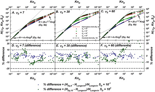
analogous to unscreened Coulomb potential model development. shows results for
in panels (a–c). On each panel, the continuum and free molecular limits are shown (dotted lines) and the simulation results converge to these limits for low and high values of
Also shown are the hard sphere fit (EquationEquation (8)
(8)
(8) ) and the Coulomb model developed in the previous section (EquationEquation (10)
(10)
(10) ) as dashed lines. For clarity, the data points of
are not shown as they are indistinguishable from
The Langevin simulation results for
are shown as discrete data points of various colors. Panels D, E, F of show the difference between the Langevin-inferred
(referred to as
) and (1) the prediction of the hard sphere fit (referred to as
) for
shown as blue triangles and (2) the prediction of Coulomb model developed in the previous section (referred to as
) for
shown as green circles. Reference lines for denoting difference levels of
and
are shown to guide the eye. Figures S4 and S5 present
and % difference values for an expanded dataset with
to further illustrate the trends shown in . For
the hard sphere fit describes the simulation results
within
nominally. Likewise, the agreement between the Langevin-inferred
and the Coulomb model (EquationEquation (10)
(10)
(10) ) is within
for all
values with a few outliers at high
We attribute this to the higher uncertainty in fitting at the end of the
range. Overall, this establishes that for
the Langevin-inferred
approaches the hard sphere fit and for
they approach the Coulomb model (EquationEquation (10)
(10)
(10) ). As
is varied between
transitions between the hard sphere fit and the Coulomb model. This variation of
is captured by the underlying variation in the
parameter introduced through EquationEquation (11)
(11)
(11) . A fit for the fit constants
that appear in EquationEquation (11)
(11)
(11) is provided in Table S1 (SI). These fits depend on
and can be used to calculate
for both the unscreened and screened Coulomb potentials.
Figure 4. Plot showing the Langevin-inferred (referred to as
) for
Panels (a–c) present
for
as data points. The continuum limit (EquationEquation (6a)
(6a)
(6a) ) and free molecular limit (EquationEquation (6b)
(6b)
(6b) ) are shown as black dotted lines. Also shown is the hard sphere fit (EquationEquation (8)
(8)
(8) ) and the unscreened Coulomb model (EquationEquation (10)
(10)
(10) ). The common legend for panels (a–c) is given in panel (b). Panels (d–f) plot the comparison of the difference between the Langevin-inferred
(referred to as
) and (1) the prediction of the hard sphere fit (referred to as
) for
shown as blue triangles and (2) the prediction of Coulomb model (referred to as
) for
shown as green circles. Reference lines for denoting difference levels of
and
are shown to guide the eye. The common legend for panels (d–f) is given at the bottom.
Results and discussion
The Langevin-inferred values have been analyzed to develop EquationEquation (10)
(10)
(10) for
in the presence of attractive unscreened (
) and screened (
finite
) Coulomb potentials between a particle and an ion. The
model developed here, valid in the limit of
based on prior evidence about the weak sensitivity of the collision kernel on
(Gopalakrishnan and Hogan Citation2011), can be used to describe charging of particles by simple atomic and molecular ions of equal or greater mass than the background gas molecules. Their application to describe charging of particles by ions that are lighter than the background gas molecules remains to be investigated. In this section, we present inter-comparison of the predictions of models available in the literature against Langevin-inferred
We choose six models from the literature along with the model developed in this paper (EquationEquation (10)
(10)
(10) ). The analytical models that represent different approaches and assumptions about the ion to gas molecule mass ratio
(
or
) discussed in the introduction: limiting sphere model pioneered by Fuchs and derived for the Coulomb potential by D’Yachkov et al. (Citation2007) assuming
the linear combination model derived by Gatti and Kortshagen (Citation2008) assuming
the expression developed by Zobnin et al. (Citation2008) based on solutions to the Boltzmann equation with an ion-neutral collision term (assuming
), and Vaulina, Repin, and Petrov (Citation2006) and Gopalakrishnan and Hogan (Citation2012) based on LD (
), Hutchinson and Patacchini (Citation2007) based on PIC calculations (assuming
) are chosen for comparison. Here, the model of Zobnin et al. (Citation2008) is analogous to models of vapor condensation derived by solving the Boltzmann equation without involving force potentials (Fuchs and Sutugin Citation1970; Loyalka Citation1982). Thus, the models chosen here for comparison represent both the limits of ion-neutral mass ratio
to assess the sensitivity of the collision kernel to the same. The models of D’Yachkov et al. (Citation2007), and Gopalakrishnan and Hogan (Citation2012), by construction, are applicable only for unscreened Coulomb potential (
) and are thus not included in the comparison for screened Coulomb potential calculations. The original formulation of Gatti and Kortshagen’s model and Hutchinson and Patacchini’s fit has a drift-diffusion expression built as the continuum or strongly collisional limit. We have replaced the continuum limit used by those authors with EquationEquation (6a)
(6a)
(6a) to ensure that those models converged to the continuum limit in the absence of systematic ion drift. For all comparisons with Langevin-inferred
these adjusted expressions of Gatti and Kortshagen’s model and Hutchinson and Patacchini’s fit are used throughout this paper. The fit developed by Hutchinson and Patacchini (Citation2007) was developed for finite electron and ion Debye lengths (as opposed to infinite Debye lengths or unscreened interactions). Following Khrapak and Morfill (Citation2008), we set an interpolation exponent in their model to 1 and apply it for finite screening lengths cases for comparison. Further, the ion to electron temperature parameter in their fit equation is set to zero to approximate a non-thermal dusty plasma, although it is noted this is not strictly true. The current model calculates the ion current to an isolated grain in the presence of neutrals with a fixed screened or unscreened Coulomb interaction potential. Hutchinson and Patacchini’s fit, however, self-consistently calculates the particle-ion interaction potential that also renders the comparison approximate to illustrate the transition of ion current from the continuum limit to the free molecular limit as a function of ion-neutral collisionality. Finally, the current model and the model put forward by Vaulina, Repin, and Petrov (Citation2006) are both based on LD and are compared on a one-to-one basis instead of comparison with models derived using other approaches. Thus, to represent the LD approach to collision kernel development, the current model is compared with other models and Langevin-inferred
The equations of the respective models used for comparison in this paper in terms of
can be found in Sec. S3, SI.
Unscreened Coulomb () potential driven particle-ion collisions
In , we present the Langevin-inferred values and model predictions for
as 4 panels. In each panel, the Langevin-inferred
for a fixed
is shown as light green circles with black outline. Predictions of the models considered are shown as dashed lines including the current model in blue, D’Yachkov et al. (Citation2007) in orange, Gatti and Kortshagen (Citation2008) in pink, Gopalakrishnan and Hogan (Citation2012) in dark green and Zobnin et al. (Citation2008) in red. Also shown are the infinitely collisional (EquationEquation (6a)
(6a)
(6a) ) and collision-less (EquationEquation (6b)
(6b)
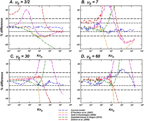
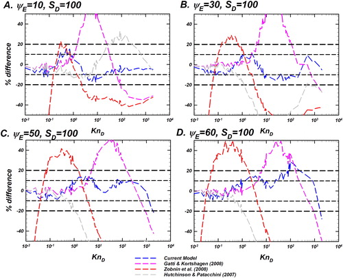
(6b) ) limits as dotted black lines. shows the % difference between the predictions of each model and the Langevin-inferred
% difference is defined as
has 4 panels that correspond to the difference of each model for corresponding value of
Immediately apparent from and is the agreement of
values with EquationEquation (6a)
(6a)
(6a) as
At low
(i. e), when the ion potential energy and thermal energy are nominally equal, the current model, D’Yachkov model and Gatti-Kortshagen’s model have very low difference within ∼5% nominally for the entire
range. However, the model developed by Gopalakrishnan and Hogan (Citation2012) has significant difference as
increases and does not converge to the collision-less limit of EquationEquation (6b)
(6b)
(6b) as
This model was designed by fitting simulation results to a rational function of
Gopalakrishnan and Hogan (Citation2012) postulated that a correct form of the capture radius (discussed in the Introduction section) should be used to calculate the diffusive Knudsen number
and used while describing attractive Coulombic collisions. Their choice of the non-dimensional capture radius of
works well only when
is well described by the continuum limit (EquationEquation (6a)
(6a)
(6a) ) as well. It can be seen from all the models agree with each other and have low difference when
is well described by the continuum limit. The
at which
departs from EquationEquation (6a)
(6a)
(6a) is dependent on
shows that for
the maximum
at which
is well described by EquationEquation (6a)
(6a)
(6a) is approximately 0.2, 2, 9, and 20, respectively. If a particle-ion collision is calculated to have a certain
depending on
the transport could be continuum or free molecular. The
value itself is only weakly dependent on
and hence, the attraction between particle and ion effectively increases the particle’s ability to capture ion from far—making the transport more continuum than if it were a hard-sphere interaction. Thus, the continuum limit represents the limit for
as
as evidenced by
datasets. For
the Gopalakrishnan and Hogan (Citation2012) model improperly approaches a false collision-less limit as
The current model, which is also built by analyzing Langevin simulations, parameterizes the underlying distribution of the particle-ion collision times (EquationEquations (10)
(10)
(10) and Equation(11)
(11)
(11) ). This approach based on the analysis of the particle-ion collision time distribution leads to differences within
as shown in for the entire
space investigated here. Physically,
represents the collision between a 2 nm particle and an
ion (300 K) at ∼100 Pa pressure. For these conditions, for a singly charged particle,
For larger particles,
decreases with size, and depending on the electron temperature in plasmas, the current model can be applied for
The flux-matching model of D’Yachkov et al. (Citation2007) does not account for ion-neutral collisions within the limiting sphere in their formalism and thereby predicts that the collision kernel
falls much faster than the
values. This makes this model inaccurate at low ion-neutral collisionalities (high
) and highly charged particles (high
). The model of Zobnin et al. (Citation2008) also has a similar mismatch in the rate at which the predictions approach the collision-less limit (EquationEquation (6b)
(6b)
(6b) ). Finally, the Gatti and Kortshagen model over predicts when compared to
Their model distinguishes between collision-less ion capture by the particle and that in which there is exactly one collision between ion and neutral gas molecule. However, for sufficiently energetic ions, more than one collision with neutrals may be necessary for its kinetic energy to become less than the attractive potential energy, thereby resulting in capture by the particle. Overall, the Gatti and Kortshagen model captures the physical trends but the degree of over-prediction increases with increasing
Figures S6 and S7 present additional
and model predictions for
to further the discussion presented here. Overall, the current model can be seen to describe the Langevin-inferred
values to within
with few instances where the difference is within
making it accurate for describing particle charging in dusty plasmas and aerosol systems in which the Debye screening length is much larger than the particle size.
Figure 5. Langevin-inferred (referred to as
shown as green circles with black outline) and the predictions of various models considered for evaluation are plotted as a function of
for
In each panel, the predictions of the unscreened Coulomb (
) model (EquationEquation (10)
(10)
(10) , blue dashed line), D’Yachkov et al. (Citation2007) in orange, Gatti and Kortshagen (Citation2008) in pink, Gopalakrishnan and Hogan (Citation2012) in dark green, and Zobnin et al. (Citation2008) in red are shown. Also shown are the infinitely collisional (EquationEquation (6a)
(6a)
(6a) ) and collision-less (EquationEquation (6b)
(6b)
(6b) ) limits as dashed black lines. For comparison of the difference between model predictions and
see .
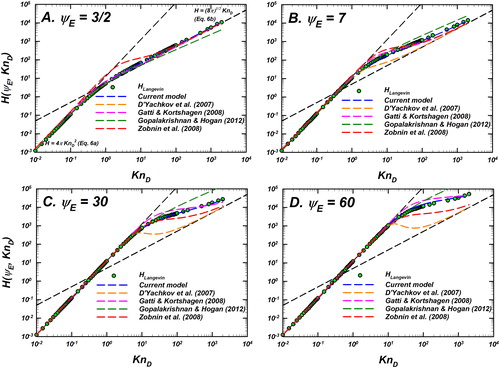
Figure 6. Comparison of the difference between the Langevin-inferred (referred to as
) and the prediction of various models as noted in the legend for
as a function of
Differences of the models considered are shown as dashed lines including the current model (EquationEquation (10)
(10)
(10) with
) in blue, D’Yachkov et al. (Citation2007) in orange, Gatti and Kortshagen (Citation2008) in pink, Gopalakrishnan and Hogan (Citation2012) in dark green, and Zobnin et al. (Citation2008) in red. The y-axis shows the % difference between the predictions of each model and
% difference is defined as
Reference lines for denoting difference levels of
and
are shown to guide the eye. This plot is to be read in conjunction with .
Screened Coulomb (finite ) potential driven particle-ion collisions
The Debye screening of individual particles by ions in the gas phase is parameterized by the normalized screening length In , S4, and S5, we showed that the effect of finite
is important in the range of
For
we find that the hard sphere fit reasonably predicts
Likewise, for
the unscreened Coulomb model describes
well.
represents the dynamic range wherein
is sensitive to both
and
Hence, we pick
and
to evaluate the accuracy of the models considered. For purpose of comparison, we select the model developed in this paper (EquationEquation (10)
(10)
(10) with
from EquationEquation (11)
(11)
(11) and fit constants from Table S2, SI), the model of Gatti and Kortshagen, model of Zobnin et al., and Hutchinson and Patacchini’s fit for comparison. shows
calculations and model predictions for
and for fixed
Likewise, shows the same for
with other parameters being identical to .
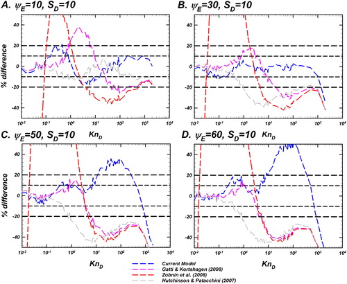
values are shown as green circles with black outline, the current model predictions in blue dashed line, Gatti and Kortshagen’s model in pink dashed line, Zobnin et al.’s model in red dashed line, and Hutchinson and Patacchini’s fit in gray dashed line. Immediately apparent is the excellent agreement of the current model and Gatti and Kortshagen’s expression with continuum limit as
Gopalakrishnan and Hogan (Citation2012) remark that the Gatti and Kortshagen’s expression was adjusted to ensure that it converges to the continuum limit that is consistent with diffusive transport of ion in the
limit (EquationEquation (6a)
(6a)
(6a) ) as opposed to their original formulation of the drift-diffusion equation. Zobnin et al.’s model does not approach the continuum limit as it is seen to make predictions for
that are non-positive as well. Both observations lead to inference that the usage of these models at moderate or higher pressures (
is problematic. In this regime, the current model describes the data to within
Zobnin et al.’s model shows improved agreement with the continuum limit at
and very good agreement with
(unscreened Coulomb as shown in , S6, and S7). Thus, Zobnin et al.’s model is prone to error at small screening lengths or high ion concentrations. The current model and Gatti and Kortshagen’s model, on the other hand, capture the trends of
quite closely. For
as can be seen from , the difference profiles of two models are similar and within
for
For
and
Gatti and Kortshagen’s model over predicts
at
to about ∼40%. The current model on the other hand has higher difference at the edge of the fitting interval near
but overall captures the data well. Zobnin et al.’s model has high difference in the low
range and has a similar difference profile to the Gatti and Kortshagen’s model at high
Hutchinson and Patacchini’s fit, for both
is similar in trend to the model of Zobnin et al. as the difference profiles of and indicate. The similarity between the two models was also seen in the comparison done by Khrapak and Morfill (Citation2008). When compared to
Hutchinson and Patacchini’s fit is lower by up to ∼40% () at
Also, the predictions of all the models compared in are reasonably close to each other. Physically,
represents high ion concentration or well-screened particles that behave more like hard spheres than charged entities. We note an inherent difference in the treatment of ion transport to the particle in the PIC calculations of Hutchinson and Patacchini. PIC takes into account the space charge effect around the particle and obtains the solution to the ion and electron concentration profile around the particle as well. The difference between PIC and LD calculations reveal the need for further work to probe the effect of space charge as well as the complex electrostatic potential around the particle, as noted in the Introduction. Among the models compared, including the model developed in this paper, Hutchinson and Patacchini’s model is the only approach that takes into account the floating potential on the particle and interactions between ions and electrons in calculating ion transport to the grain. While we have shown a reasonable description of the collision kernel for isolated particle-ion interactions without other charges being present in the vicinity, the difference between Hutchinson and Patacchini’s fit and other models reveal a further need to parameterize the space charge effect. Based on this we conclude that in high ion concentration environments, Gatti and Kortshagen’s model and the current model can be reasonably used to calculate
for the entire
range for dilute space charge environments (
) wherein ion-ion interactions can be ignored while still considering screening of particle charge. More sophisticated treatment of the particle potential will be presumably necessary to expand the applicability of LD-based models to high concentration of space charges (
). Figures S10 and S11 also show similar results of
and model predictions for lower
values such as
Figure 7. Langevin-inferred (referred to as
shown as green circles with black outline) and the predictions of various models considered for evaluation are plotted as a function of
for
and a fixed
In each panel, the predictions of the unscreened Coulomb model (EquationEquation (10)
(10)
(10) , blue dashed line), Gatti and Kortshagen (Citation2008) in pink, Zobnin et al. (Citation2008) in red and Hutchinson and Patacchini (Citation2007) in gray are shown. Also shown are the infinitely collisional (EquationEquation (6a)
(6a)
(6a) ) and collision-less (EquationEquation (6b)
(6b)
(6b) ) limits as black dashed lines. For comparison of the difference between model predictions and
see .
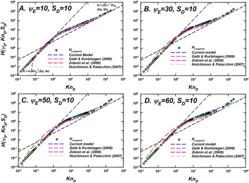
Figure 8. Comparison of the difference between the Langevin-inferred (referred to as
) and the prediction of various models as noted in the legend for
and a fixed
Differences of the models considered are shown as dashed lines including the current model (EquationEquation (10)
(10)
(10) ) in blue, Gatti and Kortshagen (Citation2008) in pink, Zobnin et al. (Citation2008) in red, and Hutchinson and Patacchini (Citation2007) in gray. The y-axis shows the % difference between the predictions of each model and
% difference is defined as
Reference lines for denoting difference levels of
and
are shown to guide the eye. This plot is to be read in conjunction with .
At the differences between predictions and
are lower than the previous case and the current model and Gatti and Kortshagen’s model capture the data quite well. As seen in , the two models capture the rise and fall of the
values and their approach towards the free molecular limit of EquationEquation (6b)
(6b)
(6b) as
confirms the agreement as the difference is within
throughout the
range investigated. Zobnin et al.’s model has a systematic error built in it at intermediate and low
values. For
Hutchinson and Patacchini’s fit is consistently lower than
(). Beyond
where the predictions of the model begin to diverge from
up to a factor of 2 lower, as seen from the difference in . Additional data to support this observation is presented in Figures S10 and S11. Overall, the current model leads to a difference of ∼
for
for all
values (0.01–2000). For
it leads to good agreement (∼
for up to
Between 200 and 2000, the difference increases up to ∼50% due to poor quality of curve fitting in this range. However, that is readily redressed by the fact that for
is well described by the hard sphere fit of EquationEquation (8)
(8)
(8) , as evidenced in , S4, and S5. Gatti and Kortshagen’s model does not differ significantly from
and current model’s predictions. That model, however has a ∼40% over prediction at mid
range (
). Combined with the fact that the original formulation presented in their paper has a drift-diffusion expression built as the continuum or strongly collisional limit, this makes the model problematic to apply at intermediate or moderate pressure dusty plasmas.
Figure 9. Langevin-inferred (referred to as
shown as green circles with black outline) and the predictions of various models considered for evaluation are plotted as a function of
for
and a fixed
In each panel, the predictions of the unscreened Coulomb model (EquationEquation (10)
(10)
(10) , blue dashed line), Gatti and Kortshagen (Citation2008) in pink, Zobnin et al. (Citation2008) in red, and Hutchinson and Patacchini (Citation2007) in gray are shown. Also shown are the infinitely collisional (EquationEquation (6a)
(6a)
(6a) ) and collision-less (EquationEquation (6b)
(6b)
(6b) ) limits as black dashed lines. For comparison of the difference between model predictions and
see .
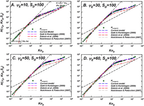
Figure 10. Comparison of the difference between the Langevin-inferred (referred to as
) and the prediction of various models as noted in the legend for
and a fixed
Differences of the models considered are shown as dashed lines including the current model (EquationEquation (10)
(10)
(10) ) in blue, Gatti and Kortshagen (Citation2008) in pink, Zobnin et al. (Citation2008) in red, and Hutchinson and Patacchini (Citation2007) in gray. The y-axis shows the % difference between the predictions of each model and
% difference is defined as
Reference lines for denoting difference levels of
and
are shown to guide the eye. This plot is to be read in conjunction with .
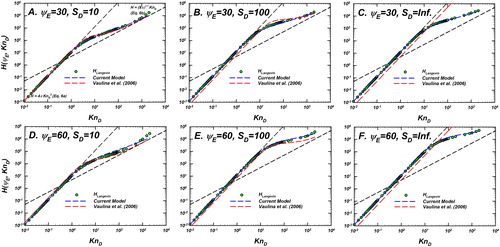
The model developed in this paper and the model of Vaulina, Repin, and Petrov (Citation2006), both based on LD calculations of particle-ion collisions, are compared to illustrate the similarity in their predictions and formulation. shows the predictions of the current model (blue dashed line) and Vaulina et al.’s expression (red dashed line) along with values (green filled circles with black outline). In panels A, B, C, for
and
the two models are qualitatively similar—the transition of
from the continuum limit (EquationEquation (6a)
(6a)
(6a) ) onto the collisionless/free molecular limit is seen around similar
value. However, for the case of unscreened Coulomb interaction (
), Vaulina et al.’s expression predicts
to be equal to the continuum limit (only differing by a constant), as is seen from . the same is true at
as can be seen from panels (d–f). For finite values of
the two models qualitatively predict the same variation of
while for unscreened Coulomb interactions (low ion concentrations, finite
), Vaulina et al.’s fit does not approach the OML limit as the disagreement with
shows. Nevertheless, the similarity in the methodology of constructing the two models is the reason for qualitative, if not quantitative similarity.
Figure 11. Langevin-inferred (referred to as
shown as green circles with black outline) and the predictions of Langevin dynamics based models—the current model and the model of Vaulina, Repin, and Petrov (Citation2006) are plotted as a function of
for
and
In each panel, the predictions of the current model (EquationEquation (10)
(10)
(10) , blue dashed line) and Vaulina, Repin, and Petrov (Citation2006) (red dashed line) are shown. Also shown are the infinitely collisional (EquationEquation (6a)
(6a)
(6a) ) and collision-less (EquationEquation (6b)
(6b)
(6b) ) limits as black dashed lines.
Finally, we note that among the models that were compared with each other for both the unscreened and screened Coulomb potentials, the closest agreement in the predictions are found between the model presented in this paper and Gatti and Kortshagen’s model. It may be recalled that the model derived here based on Langevin tracking of ion trajectories is valid in the limit of and that Gatti and Kortshagen’s model is derived assuming
The other models compared here also assume
Similar to Gopalakrishnan and Hogan (Citation2011), we find here that models derived assuming
and
lead to qualitatively similar predictions (within ∼40% maximum deviation). Further work will be necessary to probe the sensitivity of the collision kernel to
for which the current work provides some justification to believe, if any, that the collision kernel only weakly depends on
Conclusions
We have used LD to simulate Coulomb potential driven spherical particle-ion collisions and the associated collision kernel or ion flux coefficient. LD provides an approximate, yet physical, treatment of potential driven collision across the entire transition regime of ion-neutral collisionality. The Gumbel distribution accurately describes the underlying distribution of the particle-ion collision times and the non-dimensional ion flux coefficient
The effect of particle screening has been parameterized by calculating
For the unscreened Coulomb potential, the current model and four selected models from the literature were compared against the Langevin-inferred
For the screened Coulomb potential, the current model and two other models were compared against the Langevin-inferred
Finally, we present a self-contained model for the calculation of the ion flux coefficient
Supplemental Material for this article can be accessed at https://doi.org/10.1080/02786826.2019.1614522.
Download Zip (4.1 MB)Acknowledgments
We are indebted to our three anonymous reviewers and to our editor, Dr. Yannis Drossinos, all of whose constructive criticism greatly helped shape our thinking on this topic.
References
- Adachi, M., Y. Kousaka, and K. Okuyama. 1985. Unipolar and bipolar diffusion charging of ultrafine aerosol-particles. J. Aerosol Sci. 16 (2):109–123. doi: 10.1016/0021-8502(85)90079-5.
- Adachi, M., K. Okuyama, H. Kozuru, Y. Kousaka, and D. Y. H. Pui. 1989. Bipolar diffusion charging of aerosol particles under high particle/ion concentration ratios. Aerosol Sci. Technol. 11 (2):144–156. doi: 10.1080/02786828908959307.
- Allen, J. E. 1992. Probe theory—The orbital motion approach. Phys. Scr. 45 (5):497–503. doi: 10.1088/0031-8949/45/5/013.
- Autricque, A., S. A. Khrapak, L. Couëdel, N. Fedorczak, C. Arnas, J. M. Layet, and C. Grisolia. 2018. Electron collection and thermionic emission from a spherical dust grain in the space-charge limited regime. Phys. Plasmas 25 (6):063701. doi: 10.1063/1.5032153.
- Bonitz, M., C. Henning, and D. Block. 2010. Complex plasmas: A laboratory for strong correlations. Rep. Prog. Phys. 73 (6):066501. doi: 10.1088/0034-4885/73/6/066501.
- Bricard, J. 1962. La fixation des petits ions atmosphériques sur les aérosols ultra-fins. Geofisica Pura e Applicata 51 (1):237–242. doi: 10.1007/BF01992666.
- Bystrenko, O., and A. Zagorodny. 1999. Critical effects in screening of high-z impurities in plasmas. Phys. Lett. A 255 (4–6):325–330. doi: 10.1016/S0375-9601(99)00137-1.
- Chandrasekhar, S. 1943. Stochastic problems in physics and astronomy. Rev. Mod. Phys. 15 (1):1–89. doi: 10.1103/RevModPhys.15.1.
- Chaudhuri, M., A. V. Ivlev, S. A. Khrapak, H. M. Thomas, and G. E. Morfill. 2011. Complex plasma—The plasma state of soft matter. Soft Matter 7 (4):1287–1298. doi: 10.1039/C0SM00813C.
- Coles, S. 2001. An introduction to statistical modeling of extreme values. Berlin: Springer.
- D’Yachkov, L. G., A. G. Khrapak, S. A. Khrapak, and G. Morfill. 2007. Model of grain charging in collisional plasmas accounting for collisionless layer. Phys. Plasmas 14 (4):042102.
- Dahneke, B. E. 1983. Simple kinetic theory of Brownian diffusion in vapors and aerosols. In Theory of dispersed multiphase flow, ed. R. E. Meyer, New York: Academic Press.
- Daugherty, J. E., R. K. Porteous, and D. B. Graves. 1993. Electrostatic forces on small particles in low-pressure discharges. J. Appl. Phys. 73 (4):1617–1620. doi: 10.1063/1.353194.
- Daugherty, J. E., R. K. Porteous, M. D. Kilgore, and D. B. Graves. 1992. Sheath structure around particles in low‐pressure discharges. J. Appl. Phys. 72 (9):3934–3942. doi: 10.1063/1.352245.
- Ermak, D. L., and H. Buckholz. 1980. Numerical integration of the Langevin equation: Monte Carlo simulation. J. Comput. Phys. 35 (2):169–182. doi: 10.1016/0021-9991(80)90084-4.
- Filippov, A. V. 1993. Charginf of aerosol in the transition regime. J. Aerosol Sci. 24 (4):423–436. doi: 10.1016/0021-8502(93)90029-9.
- Fortov, V. E., A. V. Ivlev, S. A. Khrapak, A. G. Khrapak, and G. E. Morfill. 2005. Complex (dusty) plasmas: Current status, open issues, perspectives. Phys. Rep. 421 (1–2):1–103. doi: 10.1016/j.physrep.2005.08.007.
- Fortov, V. E., O. F. Petrov, A. D. Usachev, and A. V. Zobnin. 2004. Micron-sized particle-charge measurements in an inductive RF gas-discharge plasma using gravity-driven probe grains. Phys. Rev. E 70:046415.
- Friedlander, S. K. 2000. Smoke, dust, and haze: Fundamentals of aerosol dynamics. New York: Oxford University Press.
- Fuchs, N. A. 1963. On the stationary charge distribution on aerosol particles in a bipolar ionic atmosphere. Geofis. Pura Appl. 51:185–193. doi: 10.1007/BF01993343.
- Fuchs, N. A. 1964. The mechanics of aerosols. New York: Macmillan.
- Fuchs, N. A., and A. G. Sutugin. 1970. Highly dispersed aerosols. Ann Arbor, MI: Ann Arbor Science Publishers.
- Gatti, M., and U. Kortshagen. 2008. Analytical model of particle charging in plasmas over a wide range of collisionality. Phys. Rev. E 78:046402. doi: 10.1103/PhysRevE.78.046402.
- Gelbard, F., Y. Tambour, and J. H. Seinfeld. 1980. Sectional representations for simulating aerosol dynamics. J. Colloid Interface Sci. 76 (2):541–556. doi: 10.1016/0021-9797(80)90394-X.
- Gnedenko, B. V. 1948. On a local limit theorem of the theory of probability. Usp. Mat. Nauk 3:187–194 (in Russian).
- Gopalakrishnan, R., and C. J. Hogan. 2011. Determination of the transition regime collision kernel from mean first passage times. Aerosol Sci. Technol. 45 (12):1499–1509. doi: 10.1080/02786826.2011.601775.
- Gopalakrishnan, R., and C. J. Hogan. 2012. Coulomb-influenced collisions in aerosols and dusty plasmas. Phys. Rev. E 85:026410.
- Gopalakrishnan, R., P. H. McMurry, and C. J. Hogan. 2015. The bipolar diffusion charging of nanoparticles: A review and development of approaches for non-spherical particles. Aerosol Sci. Technol. 49 (12):1181–1194. doi: 10.1080/02786826.2015.1109053.
- Gopalakrishnan, R., M. J. Meredith, C. Larriba-Andaluz, and C. J. Hogan, Jr. 2013. Brownian dynamics determination of the bipolar steady state charge distribution on spheres and non-spheres in the transition regime. J. Aerosol Sci. 63:126–145. doi: 10.1016/j.jaerosci.2013.04.007.
- Gopalakrishnan, R., T. Thajudeen, and C. J. Hogan. 2011. Collision limited reaction rates for arbitrarily shaped particles across the entire diffusive Knudsen number range. J. Chem. Phys. 135 (5):054302. doi: 10.1063/1.3617251.
- Gopalakrishnan, R., T. Thajudeen, H. Ouyang, and C. J. Hogan, Jr. 2013. The unipolar diffusion charging of arbitrary shaped aerosol particles. J. Aerosol Sci. 64:60–80. doi: 10.1016/j.jaerosci.2013.06.002.
- Goree, J. 1992. Ion trapping by a charged dust grain in a plasma. Phys. Rev. Lett. 69 (2):277–280. doi: 10.1103/PhysRevLett.69.277.
- Hagen, D. E., and D. J. Alofs. 1983. Linear inversion method to obtain aerosol size distributions from measurements with a differential mobility analyzer. Aerosol Sci. Technol. 2 (4):465–475. doi: 10.1080/02786828308958650.
- Han, B., M. Shimada, M. Choi, and K. Okuyama. 2003. Unipolar charging of nanosized aerosol particles using soft X-ray photoionization. Aerosol Sci. Technol. 37 (4):330–341. doi: 10.1080/02786820390125197.
- Hogan, C. J., L. Li, D. R. Chen, and P. Biswas. 2009. Estimating aerosol particle charging parameters using a Bayesian inversion technique. J. Aerosol Sci. 40 (4):295–306. doi: 10.1016/j.jaerosci.2008.11.008.
- Hopkins, M. B., and W. G. Graham. 1986. Langmuir probe technique for plasma parameter measurement in a medium density discharge. Rev. Sci. Instrum. 57 (9):2210–2217. doi: 10.1063/1.1138684.
- Hoppel, W. A., and G. M. Frick. 1986. Ion-aerosol attachment coefficients and the steady-state charge distribution on aerosols in a bipolar ion environment. Aerosol Sci. Technol. 5 (1):1–21. doi: 10.1080/02786828608959073.
- Hussin, A., H. G. Scheibel, K. H. Becker, and J. Porstendörfer. 1983. Bipolar diffusion charging of aerosol particles—I: Experimental results within the diameter range 4–30 nm. J. Aerosol Sci. 14 (5):671–677. doi: 10.1016/0021-8502(83)90071-X.
- Hutchinson, I. H., and L. Patacchini. 2007. Computation of the effect of neutral collisions on ion current to a floating sphere in a stationary plasma. Phys. Plasmas 14 (1):013505. doi: 10.1063/1.2431584.
- In Jeong, J., and M. Choi. 2001. A sectional method for the analysis of growth of polydisperse non-spherical particles undergoing coagulation and coalescence. J. Aerosol Sci. 32 (5):565–582. doi: 10.1016/S0021-8502(00)00103-8.
- Iza, F., and J. K. Lee. 2006. Particle-in-cell simulations of planar and cylindrical Langmuir probes: Floating potential and ion saturation current. J. Vacuum Sci. Technol. A: Vacuum Surf. Films 24:1366–1372. doi: 10.1116/1.2187991.
- Jiang, J. K., C. J. Hogan, D. R. Chen, and P. Biswas. 2007. Aerosol charging and capture in the nanoparticle size range (6–15 nm) by direct photoionization and diffusion mechanisms. J. Appl. Phys. 102 (3):034904. doi: 10.1063/1.2768061.
- Khrapak, S., and G. Morfill. 2009. Basic processes in complex (dusty) plasmas: Charging, interactions, and ion drag force. Contrib. Plasma Phys. 49 (3):148–168. doi: 10.1002/ctpp.200910018.
- Khrapak, S. A., and G. E. Morfill. 2008. An interpolation formula for the ion flux to a small particle in collisional plasmas. Phys. Plasmas 15 (11):114503. doi: 10.1063/1.3035913.
- Khrapak, S. A., S. V. Ratynskaia, A. V. Zobnin, A. D. Usachev, V. V. Yaroshenko, M. H. Thoma, M. Kretschmer, H. Höfner, G. E. Morfill, O. F. Petrov, et al. 2005. Particle charge in the bulk of gas discharges. Phys. Rev. E: Stat. Nonlinear Soft Matter Phys. 72 (1 Pt 2):016406. doi: 10.1103/PhysRevE.72.016406.
- Khrapak, S. A., P. Tolias, S. Ratynskaia, M. Chaudhuri, A. Zobnin, A. Usachev, C. Rau, M. H. Thoma, O. F. Petrov, V. E. Fortov, et al. 2012. Grain charging in an intermediately collisional plasma. Europhys. Lett. 97 (3):35001. doi: 10.1209/0295-5075/97/35001.
- Lampe, M., R. Goswami, Z. Sternovsky, S. Robertson, V. Gavrishchaka, G. Ganguli, and G. Joyce. 2003. Trapped ion effect on shielding, current flow, and charging of a small object in a plasma. Phys. Plasmas 10 (5):1500–1513. doi: 10.1063/1.1562163.
- Lampe, M., and G. Joyce. 2015. Grain-grain interaction in stationary dusty plasma. Phys. Plasmas 22 (2):023704. doi: 10.1063/1.4907649.
- Lieberman, M. A., and A. J. Lichtenberg. 2005. Principles of plasma discharges and materials processing. New York: Wiley.
- Liu, B. Y. H., and D. Y. H. Pui. 1974. Equilibrium bipolar charge distribution of aerosols. J. Colloid Interface Sci. 49 (2):305–312. doi: 10.1016/0021-9797(74)90366-X.
- Lopez-Yglesias, X., and R. C. Flagan. 2013. Ion-aerosol flux coefficients and the steady-state charge distribution of aerosols in a bipolar ion environment. Aerosol Sci. Technol. 47:688–704. doi: 10.1080/02786826.2013.783684.
- Loyalka, S. K. 1976. Brownian coagulation of aerosols. J. Colloid Interface Sci. 57 (3):578–579. doi: 10.1016/0021-9797(76)90237-X.
- Loyalka, S. K. 1982. Condensation on a spherical droplet, II. J. Colloid Interface Sci. 87 (1):216. doi: 10.1016/0021-9797(82)90384-8.
- Lushnikov, A. A., and M. Kulmala. 2004. Flux-matching theory of particle charging. Phys. Rev. E: Stat. Nonlinear Soft Matter Phys. 70 (4 Pt 2):046413. doi: 10.1103/PhysRevE.70.046413.
- Maißer, A., J. M. Thomas, C. Larriba-Andaluz, S. He, and C. J. Hogan. 2015. The mass–mobility distributions of ions produced by a Po-210 source in air. J. Aerosol Sci. 90:36–50. doi: 10.1016/j.jaerosci.2015.08.004.
- Mann, I., A. Pellinen-Wannberg, E. Murad, O. Popova, N. Meyer-Vernet, M. Rosenberg, T. Mukai, A. Czechowski, S. Mukai, J. Safrankova, et al. 2011. Dusty plasma effects in near earth space and interplanetary medium. Space Sci. Rev. 161 (1–4):1–47. doi: 10.1007/s11214-011-9762-3.
- Marlow, W. H. 1980. Derivation of aerosol collision rates for singular attractive contact potentials. J. Chem. Phys. 73 (12):6284–6287. doi: 10.1063/1.440126.
- Mayya, Y. S., and B. K. Sapra. 2002. Image forces on a collection of charged particles near conducting surfaces. J. Aerosol Sci. 33 (5):817–828. doi: 10.1016/S0021-8502(02)00038-1.
- Mazur, P., and I. Oppenheim. 1970. Molecular theory of Brownian motion. Physica 50 (2):241. doi: 10.1016/0031-8914(70)90005-4.
- McMurry, P. H. 2000. A review of atmospheric aerosol measurements. Atmos. Environ. 34 (12–14):1959–1999. doi: 10.1016/S1352-2310(99)00455-0.
- Melzer, A., M. Himpel, H. Krüger, M. Mulsow, and S. Schütt. 2018. Optical diagnostics of dusty plasmas. Plasma Phys. Control. Fusion. 61 (1).
- Merlino, R. L. 2007. Understanding Langmuir probe current-voltage characteristics. Am. J. Phys. 75 (12):1078–1085. doi: 10.1119/1.2772282.
- Molotkov, V. I., H. M. Thomas, A. M. Lipaev, V. N. Naumkin, A. V. Ivlev, and S. A. Khrapak. 2015. Complex (dusty) plasma research under microgravity conditions: Pk-3 plus laboratory on the international space station. Int. J. Microgravity Sci. Appl. 35 (3): 320302. doi: 10.15011/jasma.32.320302.
- Morfill, G. E., and A. V. Ivlev. 2009. Complex plasmas: An interdisciplinary research field. Rev. Mod. Phys. 81 (4):1353–1404. doi: 10.1103/RevModPhys.81.1353.
- Mott-Smith, H. M., and I. Langmuir. 1926. The theory of collectors in gaseous discharges. Phys. Rev. 28 (4):727–763. doi: 10.1103/PhysRev.28.727.
- Narsimhan, G., and E. Ruckenstein. 1985. The Brownian coagulation of aerosols over the entire range of Knudsen numbers: Connection between the sticking probability and the interaction forces. J. Colloid Interface Sci. 104 (2):344–369. doi: 10.1016/0021-9797(85)90044-X.
- Nefedov, A. P., G. E. Morfill, V. E. Fortov, H. M. Thomas, H. Rothermel, T. Hagl, A. V. Ivlev, M. Zuzic, B. A. Klumov, A. M. Lipaev, et al. 2003. PKE-Nefedov*: Plasma crystal experiments on the international space station. New J. Phys. 5:33. doi: 10.1088/1367-2630/5/1/333.
- Ouyang, H., R. Gopalakrishnan, and C. J. Hogan. 2012. Nanoparticle collisions in the gas phase in the presence of singular contact potentials. J. Chem. Phys. 137 (6):064316. doi: 10.1063/1.4742064.
- Porstendörfer, J., A. Hussin, H. G. Scheibel, and K. H. Becker. 1984. Bipolar diffusion charging of aerosol particles—II. Influence of the concentration ratio of positive and negative ions on the charge distribution. J. Aerosol Sci. 15 (1):47–56. doi: 10.1016/0021-8502(84)90055-7.
- Pui, D. Y. H., S. Fruin, and P. H. McMurry. 1988. Unipolar diffusion charging of ultrafine aerosols. Aerosol Sci. Technol. 8 (2):173–187. doi: 10.1080/02786828808959180.
- Pustylnik, M. Y., M. A. Fink, V. Nosenko, T. Antonova, T. Hagl, H. M. Thomas, A. V. Zobnin, A. M. Lipaev, A. D. Usachev, V. I. Molotkov, et al. 2016. Plasmakristall-4: New complex (dusty) plasma laboratory on board the international space station. Rev. Sci. Instrum. 87 (9):093505. doi: 10.1063/1.4962696.
- Ratynskaia, S., S. Khrapak, A. Zobnin, M. H. Thoma, M. Kretschmer, A. Usachev, V. Yaroshenko, R. A. Quinn, G. E. Morfill, O. Petrov, et al. 2004. Experimental determination of dust-particle charge in a discharge plasma at elevated pressures. Phys. Rev. Lett. 93:085001.
- Reischl, G. P., J. M. Mäkelä, R. Karch, and J. Necid. 1996. Bipolar charging of ultrafine particles in the size range below 10 nm. J. Aerosol Sci. 27 (6):931–949. doi: 10.1016/0021-8502(96)00026-2.
- Reischl, G. P., H. G. Scheibel, and J. Porstendörfer. 1983. The bipolar charging of aerosols: Experimental results in the size range below 20-nm particle diameter. J. Colloid Interface Sci. 91 (1):272–275. doi: 10.1016/0021-9797(83)90332-6.
- Rogak, S. N., and R. C. Flagan. 1992. Coagulation of aerosol agglomerates in the transition regime. J. Colloid Interface Sci. 151 (1):203–224. doi: 10.1016/0021-9797(92)90252-H.
- Semenov, I. L., S. A. Khrapak, and H. M. Thomas. 2015. Approximate expression for the electric potential around an absorbing particle in isotropic collisionless plasma. Phys. Plasmas 22 (5):053704. doi: 10.1063/1.4921249.
- Shukla, P. K., and B. Eliasson. 2009. Colloquium: Fundamentals of dust-plasma interactions. Rev. Mod. Phys. 81 (1):25–44. doi: 10.1103/RevModPhys.81.25.
- Stober, J., B. Schleicher, and H. Burtscher. 1991. Bipolar diffusion charging of particles in noble gases. Aerosol Sci. Technol. 14 (1):66–73. doi: 10.1080/02786829108959471.
- Stolzenburg, M. R., and P. H. McMurry. 1991. An ultrafine aerosol condensation nucleus counter. Aerosol Sci. Technol. 14 (1):48–65. doi: 10.1080/02786829108959470.
- Taccogna, F., S. Longo, and M. Capitelli. 2003. A particle-in-cell/Monte Carlo model of the Ar+ ion collection in He gas by a cylindrical Langmuir probe in the transition regime. Eur. Phys. J. Appl. Phys. 22 (1):29–39. doi: 10.1051/epjap:2003015.
- Tarasov, V. I., and M. S. Veshchunov. 2018. On the theory of bipolar charging of large aerosol particles. Aerosol Sci. Technol. 52 (7):740–747. doi: 10.1080/02786826.2018.1455964.
- Thajudeen, T., R. Gopalakrishnan, and C. J. Hogan. 2012. The collision rate of non-spherical particles and aggregates for all diffusive knudsen numbers. Aerosol Sci. Technol. 46 (11):1174–1186. doi: 10.1080/02786826.2012.701353.
- Trunec, D., M. Holík, P. Kudrna, O. Bilyk, A. Marek, R. Hippler, and M. Tichý. 2004. Monte Carlo simulations of the electron currents collected by electrostatic probes. Contrib. Plasma Phys. 44 (7–8):577–581. doi: 10.1002/ctpp.200410084.
- Varney, R. N. 1971. Mean free paths, ion drift velocities, and the Poisson distribution. Am. J. Phys. 39 (5):534–538. doi: 10.1119/1.1986207.
- Vaulina, O. S., A. Y. Repin, and O. F. Petrov. 2006. Empirical approximation for the ion current to the surface of a dust grain in a weakly ionized gas-discharge plasma. Plasma Phys. Rep. 32 (6):485–488. doi: 10.1134/S1063780X06060055.
- Veshchunov, M. S. 2010. A new approach to the brownian coagulation theory. J. Aerosol Sci. 41 (10):895–910. doi: 10.1016/j.jaerosci.2010.07.001.
- Veshchunov, M. S. 2011. A new approach to diffusion-limited reaction rate theory. J. Eng. Thermophys. 20 (3):260–271. doi: 10.1134/S1810232811030040.
- Veshchunov, M. S. 2012. Development of the new approach to the diffusion-limited reaction rate theory. J. Exp. Theor. Phys. 114 (4):631–644. doi: 10.1134/S1063776112020148.
- Veshchunov, M. S., and I. B. Azarov. 2012. Next approximation of the random walk theory for Brownian coagulation. J. Aerosol Sci. 47:70–77. doi: 10.1016/j.jaerosci.2011.12.009.
- Wiedensohler, A. 1988. An approximation of the bipolar charge-distribution for particles in the sub-micron size range. J. Aerosol Sci. 19 (3):387–389. doi. doi: 10.1016/0021-8502(88)90278-9.
- Wiedensohler, A., and H. J. Fissan. 1988. Aerosol charging in high-purity gases. J. Aerosol Sci. 19:867–870. doi: 10.1016/0021-8502(88)90054-7.
- Wiedensohler, A., E. Lutkemeier, M. Feldpausch, and C. Helsper. 1986. Investigation of the bipolar charge-distribution at various gas conditions. J. Aerosol Sci. 17 (3):413–416. doi: 10.1016/0021-8502(86)90118-7.
- Wu, J. J., and R. C. Flagan. 1988. A discrete-sectional solution to the aerosol dynamic equation. J. Colloid Interface Sci. 123:339–352.
- Yaroshenko, V. V., B. M. Annaratone, S. A. Khrapak, H. M. Thomas, G. E. Morfill, V. E. Fortov, A. M. Lipaev, V. I. Molotkov, O. F. Petrov, A. I. Ivanov, et al. 2004. Electrostatic modes in collisional complex plasmas under microgravity conditions. Phys. Rev. E 69:066401. doi: 10.1103/PhysRevE.69.066401.
- Yun, K. M., S. Y. Lee, F. Iskandar, K. Okuyama, and N. Tajima. 2009. Effect of X-ray energy and ionization time on the charging performance and nanoparticle formation of a soft X-ray photoionization charger. Adv. Powder Technol. 20 (6):529–536. doi: 10.1016/j.apt.2009.07.002.
- Zobnin, A. V., A. P. Nefedov, V. A. Sinel’shchikov, and V. E. Fortov. 2000. On the charge of dust particles in a low-pressure gas discharge plasma. J. Exp. Theor. Phys. 91 (3):483–487. doi: 10.1134/1.1320081.
- Zobnin, A. V., A. D. Usachev, O. F. Petrov, and V. E. Fortov. 2008. Ion current on a small spherical attractive probe in a weakly ionized plasma with ion-neutral collisions (kinetic approach). Phys. Plasmas 15 (4):043705. doi: 10.1063/1.2903052.