Evaluation of PM2.5 measured in an urban setting using a low-cost optical particle counter and a Federal Equivalent Method Beta Attenuation Monitor

Abstract

We present the results of a multi-season field evaluation of a low-cost optical particle counting sensor (Purple Air PA-II) that reports mass concentration of particulate matter with diameter less than 2.5 microns (PM2.5), and is part of a relatively large and growing network of microelectronic internet-of-things sensors. We assessed 16 months of PA-II PM2.5 data collected in a near-road urban setting in the humid climate of Charlotte, North Carolina. The PA-II was collocated with a Federal Equivalent Method Beta Attenuation Monitor (BAM model 1022), and with a weather station that monitored ambient relative humidity (RH) and temperature (T). We tested and used a multiple linear regression model with BAM PM2.5, RH, and T as predictors to model the reported PA-II PM2.5. The results show a 27–57% improvement in the accuracy of the PA-II PM2.5 data relative to the reference data from the BAM, with the highest percentage improvements for moderate to high RH. The methodologies in our study are broadly applicable to other field studies of low-cost monitors, and the results are a critical improvement that suggest that PA-II may indeed be suitable for air quality, health, and urban aerosol research.

Copyright © 2019 American Association for Aerosol Research

1. Introduction

Air quality is a complex part of the urban environment that is susceptible to degradation from changing emission sources including vehicular traffic, businesses, industry, and residential activities (Harrison 2018; Lewis 2018; McDonald et al. 2018). Research often concentrates on the health effects of poor air quality at the population scale (Ebenstein et al. 2017; Hoek et al. 2013) to motivate a regulatory framework to manage the permitting of stationary and mobile sources of pollution (Berger et al. 2017). Citizen science directly connects air quality data and/or data collection with individuals, and also increases the engagement of community members in aspects of their own urban environment, such as a source of air pollution, that may be causing real or perceived concerns (Snyder et al. 2013; Storksdieck et al. 2016). The rise of low-cost, readily deployable air monitoring instrumentation provides a pathway to enhance citizen science and engagement (Castell et al. 2017; Schneider et al. 2017), and potentially offer insights at finer spatial scales beyond any established regulatory monitoring network (Kaufman et al. 2017; Morawska et al. 2018). For these endeavors to be successful, low-cost devices must undergo field and lab testing over time, space, and a range of relevant pollution concentrations and weather conditions (Lewis and Edwards 2016; Williams et al. 2014; Woodall et al. 2017).

This cross-disciplinary study evaluates an internet-of-things (IoT) low-cost air monitoring sensor called the second generation Purple Air (PA-II) that measures the number concentration of particles ranging from diameters of $0.3-10\text{ µm},$ and uses this data to derive the mass concentration of particulate matter for particles with diameters less than $2.5\text{ μm}$ (PM2.5) and other size specific mass concentrations. The PA-II is built with standard IoT technologies with the main particle sensors being a pair of Plantower PMS5003 sensors (Zamora et al. 2019) referred to in the PA-II data stream as sensors A and B. The company markets the PA-II to the end-user as an off-the-shelf, low-cost (∼$200), deployable sensor package. Advantages to PA-II include no specific expertise for deployment, a company-maintained cloud server for data which precludes the need for any user-based data management infrastructure, data that can be digitally re-directed to other servers, archiving of ancillary data (such as the size-segregated particle counts) that are used to determine the reported PA-II PM2.5, and measurements of relative humidity (RH) and temperature (T). All of this, combined with the open source data collection and low instrument cost, is perhaps the main reason there are over 2000 PA-IIs deployed worldwide by public organizations and private citizens as of August 2018 (https://www.purpleair.com/map). While interest in the PA-II and similar IoT devices has grown, scientific communities and regulatory agencies continue to try and understand the details of how the reported data compares with established methods of monitoring PM2.5 (Crilley et al. 2018; Lewis and Edwards 2016; Zamora et al. 2019).

The PA-II measures number concentration for different size ranges by relating the optical scattering by suspended particles in the air drawn into the PA-II sample volume (Northcross et al. 2013; Zamora et al. 2019), but the specific calculations used to aggregate and convert the number concentrations into a single mass concentration such as PM2.5 are not available. Fundamentally, it is well understood that this conversion from number to mass concentration is not trivial (Hegg and Kaufman 1998; Reid et al. 2005; Seinfeld and Pandis 2016) since there is sensitivity to assumptions about the mass density of particles in the sample population, uncertainty in the size-segregated number concentration measurements, and to variable physical and chemical properties of the particles that impact light scattering. Furthermore, the particle size distribution, which is sometimes referred to as an aerosol size distribution (Seinfeld and Pandis 2016), is sensitive to ambient RH (Hegg, Larson, and Yuen 1993).

High RH has been discussed as a barrier in a number of studies of low-cost instrumentation (Carvlin et al. 2017; Crilley et al. 2018; Rai et al. 2017). PA-IIs, for example, measure number concentrations of particles with diameters as small as $0.3\text{ μm},$ but the real atmosphere also has significant numbers of particles with even smaller diameters (Kumar et al. 2014; Posner and Pandis 2015). Scientific or regulatory research usually measures aerosol properties (number, mass) of a “dried” air sample (Kotchenruther and Hobbs 1998; Magi and Hobbs 2003; Magi et al. 2005; Petters and Kreidenweis 2007). In practice, drying the air is usually accomplished by heating the sample inlet that draws in ambient air, evaporating the liquid water condensed onto the particle, and then isolating the water condensate from the air stream before sampling. A target sample RH of a heated air sample would be around 30% under controlled conditions. The dried air PM2.5 mass is the metric that is evaluated in scientific and regulatory studies since water vapor and RH are highly variable diurnally, seasonally, and spatially.

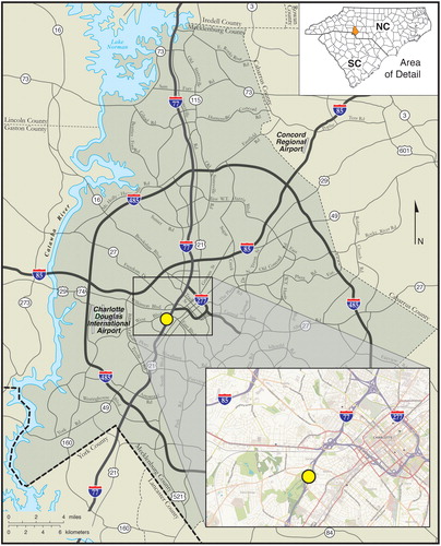
We used the PA-II to measure PM2.5 in the near-road urban environment in Charlotte, North Carolina (Figure 1), from March 2017 through June 2018. The PA-II was collocated with a Beta-Attenuation Monitor (BAM; Model 1022 manufactured by MetOne, Inc., Grants Pass, Oregon) that is used as a Federal Equivalent Method (FEM) to measure PM2.5 for compliance assessment in the Charlotte region. In addition to PM2.5 data, the collocation site also included a weather station for monitoring ambient T, RH, and wind. All raw PA-II and BAM data are publicly available, as are the processed data specific to this study.

Figure 1. Map of sampling location showing Mecklenburg County in south-central North Carolina, major freeways and roads, and the airport relative to the collocation site at the Remount Road sampling station (yellow dot) maintained by the Mecklenburg County Air Quality office. Note that the downtown Charlotte area surrounded by the 77 and 277 freeways is located about 1–2 miles east-northeast of the Remount Road station.

The fundamental question we explore is how PA-II reported PM2.5 compares with reference PM2.5 data from one collocated BAM 1022 over the period of 16 months of nearly continuous sampling. We discuss steps to quality control the PA-II data, evaluate the limit of detection (LOD), and present comparisons with BAM data that lead to a correction method that accounts for the role of ambient RH and T variability. Our flexible methodology can be used to post-process off-the-shelf PA-II PM2.5 data, and our results show that corrected PA-II PM2.5 are over 45% more accurate when compared with reference data from the BAM. We also show that the PA-II is a reliable field instrument; for the 16 months referred to in this study, PA-II required no parts replacement or re-calibration, and the device accuracy did not degrade significantly. Our findings increase the scientific and stakeholder relevance of the low-cost air quality data (Morawska et al. 2018) collected in urban and non-urban environments.

2. Methods

2.1. Sampling

The PA-II microelectronics are contained in a palm-sized plastic cap that acts as a shield from precipitation and direct sunlight – images are available at the Purple Air website. Our off-the-shelf sensor has been sampling continuously since March 2017, and the plastic protective cap is exposed to direct sunlight for significant parts of each day in our sample location. We have not undertaken any maintenance of the PA-II. A weatherproof power cord extends from the electronics, and in addition to the first Plantower particle counter (Sensor A), the plastic cap houses a second identical Plantower sensor (Sensor B) counter, Wi-Fi transmitter, hygrometer for measuring RH, and thermometer for measuring T. These RH and T data are related to ambient RH and T, but are not the same. We discuss this difference, the data from the additional particle counter, the role of RH and T variability, and the reliability of the sensor below.

The PA-II was positioned about 2 m from the sampling inlet of the BAM 1022, the latter of which is maintained by Mecklenburg County Air Quality (MCAQ) staff scientists. A full description of the BAM 1022 and its standard operations can be found at the manufacturer’s website (https://metone.com/air-quality-particulate-measurement/regulatory/bam-1022/). In November 2013, the MetOne BAM-1022 was designated by the US EPA as an FEM for the collection of PM2.5 (Gobeli, Schloesser, and Pottberg 2008). Routine calibration and verification activities by MCAQ include flow calibration, temperature calibration, pressure calibration, and relative humidity calibration every 6 months, flowrate/temperature/pressure verification every month, and flowrate/temperature/pressure audit quarterly.

The Remount station is 3.2 km southwest of the urban center of Charlotte, adjacent to a major freeway (I-77 South) on a street called Remount Road (Figure 1). Because of this particular location in the Charlotte area, we refer to the instruments as the Remount PA-II and Remount BAM, and note that the Remount BAM serves as the reference data set in this study. The Remount station also includes a weather station that reports hourly relative humidity (Met One Model 083E-35), temperature (R.M. Young Model 41432VC), wind speed and wind direction (Met One Model 50.5H). We explicitly consider the influence of relative humidity and temperature in our analysis.

2.2. Data processing

The Remount PA-II sensor was deployed in March 2017 and sampled continuously through June 2018, with values recorded about once every 90 s. In our study, we used the PA-II PM2.5 data field called “PM2.5_CF_ATM” which is available for both the PM2.5 sensors in the PA-II package, and uses the “atmospheric” setting for particle density to derive PM2.5 from the measured number concentrations (Zamora et al. 2019). Hourly PM2.5 and weather data from the Remount BAM and weather station were obtained from the public AirNow website.

For comparison with BAM data, we averaged raw PA-II data to hourly increments applying quality control filters to the raw ∼90 s data. First, when the reported values of PA-II PM2.5 are less than about $5\text{ μg }{\mathrm{m}}^{-3},$ there is often an artificially repeated value in many consecutive time steps of reported data. We assume this is an artifact because of the very low concentrations being sampled but also because it is statistically unlikely that the number of particles remains exactly the same from one 90 s sample to the next. We chose to exclude any repeated values within three time-steps. The second step is to calculate hourly averaged PA-II data using the ∼90 s quality-controlled raw data. We required a minimum of 20 min of the hour to be reported for a valid hourly average. Missing data from PA-II arises from quality controlling for repeated-values artifacts described above, instrument downtime from power or internet loss, and network downtime from the manufacturer, but in total only accounts for 4.5% of the 11,832 h of data in the sample period. The BAM data are distributed as hourly averages that are produced with a 75% completeness requirement (45 min of the 60 min). This is stricter than what we applied to PA-II, but this choice had minimal impact on our final results.

After the data from March 2017 through June 2018 were downloaded and averaged to hourly time scales, we then considered the hourly LOD. We adopt the BAM 1022 manufacturer-determined hourly LOD of $2.4\text{ μg }{\mathrm{m}}^{-3}$ (https://metone.com/air-quality-particulate-measurement/regulatory/bam-1022/). Since PA-II LOD is not well established, we surmise that the PA-II LOD is greater than the BAM 1022 LOD (a lower estimate), and use segmented regression (also known as a broken stick regression), a standard statistical method, to estimate a level of PM2.5 above which we are confident that we have signal and not random data. Using hourly PA-II and BAM PM2.5 in the segmented regression, we estimate the upper limit of PA-II LOD as $7.5\text{ μg }{\mathrm{m}}^{-3}$ (Figure S1). Acknowledging that this is an overly simplistic field-determined LOD, we nevertheless estimate PA-II hourly LOD as the average of our lower and upper estimate, or $5.0\text{ μg }{\mathrm{m}}^{-3},$ which at least is consistent with an LOD analysis using similar IoT sensors (Wang et al. 2015). For the hourly PM2.5 comparisons and the regression analysis described below, all BAM data less than LOD of $2.4\text{ μg }{\mathrm{m}}^{-3}$ or PA-II less than LOD of $5.0\text{ μg }{\mathrm{m}}^{-3}$ are excluded. In total, 612 h of BAM PM2.5 data and 1740 h of PA-II PM2.5 were less than their respective LODs, or about 20% of the over 11,000 h remaining after the first quality control filters.

The final data processing step is to analyze the comparisons only when we have a sufficient number of observations to avoid drawing conclusions about undersampled values of reported PM2.5, which also weaken the assumption of normality in the residuals discussed below. In particular, while we collected field data across a wide range of weather conditions, the reported PM2.5 values were available across a more limited range (Figure S2) owing mainly to the relatively low PM2.5 concentrations in our sample location. Referring to the reference BAM PM2.5 data, both before and after LOD is applied to the data, 99% of the sampled data was for PM2.5 less than $30\text{ μg }{\mathrm{m}}^{-3}.$ For uncorrected PA-II PM2.5, 99% of the sampled data was for PM2.5 less than $50\text{ μg }{\mathrm{m}}^{-3}.$ For this study, we limit the analysis to include only hourly averaged values when PA-II PM2.5 is less than $50\text{ μg }{\mathrm{m}}^{-3},$ which excludes 60 h of the data.

3. Results

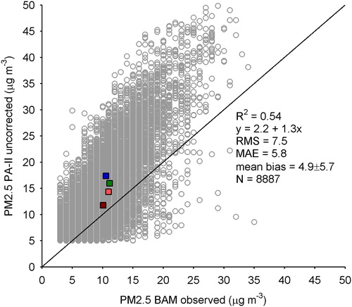
Following the quality-control steps, and the application of the hourly LOD for each instrument, a simple linear regression of hourly PA-II PM2.5 onto BAM PM2.5 shows that PA-II is biased high (Figure 2) which is consistent with similar collocation and lab comparisons (Holstius et al. 2014; Kelly et al. 2017; Wang et al. 2015; Zamora et al. 2019). Root-mean-squared error (RMS) and the mean absolute error (MAE) are the metrics we use in this study to summarize this and other comparisons; MAE tends to be less influenced by outliers but RMS is a more common calculation. RMS and MAE for the comparison in Figure 2 are $7.5$ and $5.8\text{ μg }{\mathrm{m}}^{-3},$ but the small colored squares show how the comparison depends on the ambient RH. As RH increases from 30% to 90%, RMS increases linearly from $5.0$ to $8.8\text{ μg }{\mathrm{m}}^{-3}$ and MAE from $3.7$ to $7.1\text{ μg }{\mathrm{m}}^{-3}.$

Figure 2. Hourly PM2.5 reported by PA-II versus BAM 1022, where the lower limit of detection (LOD) of $5\text{ μg }{\mathrm{m}}^{-3}$ applied to the PA-II data and LOD of $2.4\text{ μg }{\mathrm{m}}^{-3}$ for BAM 1022. The data are also limited to raw PA-II PM2.5 less than $50\text{ μg }{\mathrm{m}}^{-3},$ due to lack of available data at these high concentrations from the particular sample location. The squares are the average PM2.5 values for RH of 0–40% (dark red), 40–60% (light red), 60–80% (green), 80–100% (blue), showing that the high bias increases as a function of RH. Black line is the one-to-one comparison.

Other factors, such as weather, play a role in understanding the values reported by a low-cost sensor (Morawska et al. 2018), so we investigated multiple linearity by comparing PA-II and BAM PM2.5, PA-II and ambient RH, and PA-II and ambient T using a simple linear regression, along with histograms showing how often hourly PA-II PM2.5 was sampled as a function of the same three variables (Figure S3). Over the 16 months of sampling, ambient temperature (T) and relative humidity (RH) from the Remount Road weather station varied from $-11.5°\mathrm{C}$ to $35.6°\mathrm{C}$ with a mean and standard deviation of $16\pm 9°\mathrm{C},$ and from $30\mathrm{\%}$ to $100\mathrm{\%}$ with a mean and standard deviation of $66\mathrm{\%}\pm 22\mathrm{\%}.$ As is typical of the climate of North Carolina, RH was elevated in every season of the year, with 75% of the hourly data recording RH > 47%.

The linear dependence of PA-II PM2.5 on BAM PM2.5 and RH, and to a lesser degree on ambient T are the basis for defining the predictors of PA-II PM2.5 in the following multiple linear regression (MLR) model: (1) $$\mathrm{PM}{2.5}_{\mathrm{PA}-\mathrm{II}}=a_0+a_1\mathrm{P}\mathrm{M}{2.5}_{\mathrm{BAM}}+a_2\mathrm{R}\mathrm{H}+a_3\mathrm{T},$$(1) where $a_0,$ $a_1,$ $a_2,$ and $a_3$ are the MLR fit coefficients, $\mathrm{PM}{2.5}_{\mathrm{PA}-\mathrm{II}}$ and $\mathrm{PM}{2.5}_{\mathrm{BAM}}$ are in units of $\text{μg }{\mathrm{m}}^{-3},$ $\mathrm{RH}$ is in units of percent, and $\mathrm{T}$ is in units of Kelvin. The goal of the model is to adjust the hourly $\mathrm{PM}{2.5}_{\mathit{PA}-\mathit{II}}$ to better match the reference PM2.5 from BAM. The MLR fit using all available and valid predictor data (i.e., Figure S3) with PM2.5 from PA-II sensor A produces $a_0=-25.55\pm 1.87,$ $a_1=1.25\pm 0.01,$ $a_2=0.099\pm 0.003,$ and $a_3=0.072\pm 0.006$ (plus/minus indicates standard deviation in the regression coefficients). The coefficient of determination ($R^2$) for the model is $0.60,$ which suggests that about 60% of the variability of $\mathrm{PM}{2.5}_{\mathrm{PA}-\mathrm{II}}$ about the mean value is explained by the MLR model.

The statistical strength of the MLR model itself is partly justified by the low uncertainty of the fit coefficients and relatively high $R^2$ value, but we also evaluate the residuals of the model, and the overall effectiveness of the model using RMS and MAE. The residuals violate the constant variance assumption underlying the regression but have nearly normal distribution about zero (Figure S4) suggesting that there are no significant predictors missing from the model, but that uncertainty is likely underestimated for higher predicted PM2.5 values. Typically, non-constant variance is overcome by transforming the predictand in the regression model (i.e., log or box-cox transform). We explored this, but found that the model using a transformed predictand drifted to negative PM2.5 values that were difficult to reconcile with real particle physics (negative mass is physically meaningless, even though it is statistically acceptable). The corrected $\mathrm{PM}{2.5}_{\mathrm{PA}-\mathrm{II}}$ is calculated by inverting the MLR as (2) $$\mathrm{PM}{2.5}_{\mathrm{PA}-\mathrm{II},\mathrm{ }\mathrm{corrected}}=\frac{\left(\mathrm{PM}{2.5}_{\mathrm{PA}-\mathrm{II}}-a_0-a_2\mathrm{R}\mathrm{H}-a_3\mathrm{T}\right)}{a_1}.$$(2)

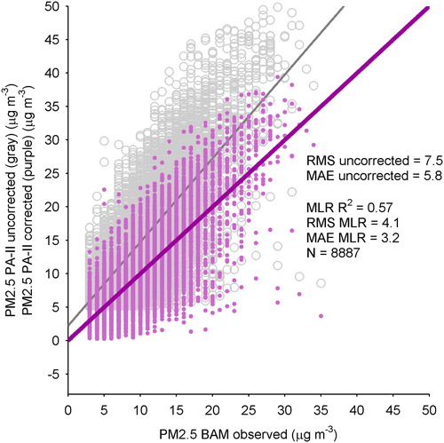
The corrected $\mathrm{PM}{2.5}_{\mathrm{PA}-\mathrm{II}}$ is plotted in Figure 3, and the MAE and RMS compared with reference $\mathrm{PM}{2.5}_{\mathrm{BAM}}$ are $3.2$ and $4.1\text{ μg }{\mathrm{m}}^{-3}.$ Compared with the statistics in Figure 2, the RMS and MAE decrease by about 45%, even though 40% of the variability of the $\mathrm{PM}{2.5}_{\mathrm{PA}-\mathrm{II}}$ is unexplained by the model. A regression model that excludes ambient RH and T also improves the absolute comparison, but by about 41%. We explore the role of RH and T variability below.

Figure 3. Comparison of hourly uncorrected PA-II PM2.5 versus BAM observed PM2.5 (gray) and corrected PA-II PM2.5 versus BAM observed PM2.5 (purple). Gray and purple lines are the simple linear regression of the gray circles and purple dots, respectively. Statistics included are the RMS and MAE for the uncorrected and corrected (MLR) data, and the number of data points (N) in the regression.

To understand the sensitivity of the MLR fit, we use Monte Carlo cross-validation to test model stability and effectiveness at capturing values outside of the data used to determine the model coefficients. Specifically, we randomly select 90% of the full data to use in the MLR model, and then use the remaining 10% as an out-of-sample validation data set. This randomized subsetting produces a new set of fit coefficients for every permutation (i.e., a Monte Carlo process). The fit coefficients from each permutation are then used with the validation subset of the data to produce a set of predicted PM2.5 values. These and the model fit coefficients are then evaluated in a similar way as the results from the full model.

The RMS, MAE, $R^2,$ and the three variable-specific fit coefficients are plotted as histograms of the results of the 10,000 Monte Carlo permutations (Figure S5). The mean and standard deviation of the fit coefficients from the Monte Carlo cross-validation are $a_0=-25.55\pm 0.57,$ $a_1=1.255\pm 0.005,$ $a_2=0.0992\pm 0.0009,$ and $a_3=0.072\pm 0.002,$ and the corresponding mean and standard deviation of the goodness-of-fit metrics are $R^2=0.57\pm 0.03,$ $\mathrm{RMS}=4.1\pm 0.1 \text{μg }{\mathrm{m}}^{-3},$ and $\mathrm{MAE}=3.20\pm 0.08\text{ μg }{\mathrm{m}}^{-3}.$ These values are all within one standard deviation of the analogous values using the full dataset (Figure 3) suggesting very little sensitivity of the MLR model to randomized subsetting of the input data. This establishes the robustness of the MLR model for use as a correction methodology.

The PA-II housing includes additional IoT devices to measure RH and T as well as the second particle counter (sensor B) as a way to monitor internal consistency with PA-II sensor A PM2.5, and all data are reported/archived online alongside the secondary number concentration data. When PA-II RH and T are compared with the ambient RH and T measured by the weather station at the Remount measurement station (Figure S6), a simple linear regression suggests that while most of the variability about the dependent variable is explained by a linear model, there is a significant high bias in T measured by PA-II and low bias of RH relative to the weather station data. Likely, these biases arise from the proximity of the IoT sensors for RH and T being located within the plastic cap that also contains the two particle sensors and WiFi transmitter. T is responding to ambient T but then elevated by about 25% on average (or about $6°\mathrm{C}$) due to the waste heat of the other IoT devices. Analogously, RH is biased low by about 16% because the T is elevated. The PA-II heats and dries the air (lowers the RH) in the sample chamber relative to the ambient conditions, but fortunately the bias is systematic. The MLR model compiled using RH and T from the PA-II (Figure S7) produces strong results (Figure S8), but with different fit coefficients (Figure S9). The PM2.5 data from PA-II sensor B are linearly related to the PA-II PM2.5 data from sensor A that this study focuses on (e.g., Figure 3), so any differences between the particle sensors are accounted for in the MLR model coefficients with no loss in overall accuracy of the correction (Figure S10). We discuss these MLR results using different predictands and predictors below.

4. Discussion

Correcting PA-II PM2.5 data to best match BAM is strongly dependent on the linear bias of PA-II relative to the reference values, but we also show that ambient RH and, to a lesser degree, ambient T play a role. Physically, this is consistent with considerations of the aerosol size distribution response to varying RH conditions (Hegg, Larson, and Yuen 1993; Magi and Hobbs 2003; Petters and Kreidenweis 2007) relative to the range of particle sizes that are detectable with the microelectronics of the PA-II. PA-II only slightly heats the sampled air relative to ambient conditions (Figure S6) as opposed to reducing RH to a controlled value (Kotchenruther and Hobbs 1998; Reid et al. 2005). This, we suggest, has consequences in precisely which part of the particle size distribution the PA-II is counting from. Water mass that condenses on a particle causes each to swell to a larger diameter, including particles that are less than the lowest detectable diameter of the PA-II of $0.3\text{ μm}.$ This region of the aerosol size distribution transitions from the Accumulation mode (diameters of about$\mathrm{ }0.1-2\text{ μm}$) to the Aitken mode (particles with diameters ranging from about $0.02-0.2\text{ μm}$) and ultrafine mode (particles with diameters less than $0.1\text{ μm}$) (Posner and Pandis 2015; Seinfeld and Pandis 2016). Numerous field studies that measure the aerosol size distribution show that Aitken and ultrafine modes typically contain far greater numbers of particles than the Accumulation mode of the size distribution. As water condenses onto sub-Accumulation model particles, they can swell to well over 100–200% of their dry diameter depending on the solubility (Gao et al. 2003; Koehler et al. 2006; Kreidenweis et al. 2005; Magi and Hobbs 2003; Magi et al. 2005). This is often referred to as a humidification factor or hygroscopic growth factor (Hegg et al. 1997) and is part of, for example, the monitoring suite for global aerosol observation networks (Sherman et al. 2015).

The protocol for heating the air sample to reduce RH requires a meticulously designed sampling system (Sherman et al. 2015) that is beyond the needs of most citizen scientists using air monitors such as the PA-II. However, there are repeated instances in literature related to low-cost sampling systems that allude to the confounding role of RH in assessing comparisons of PM2.5 (Holstius et al. 2014; Snyder et al. 2013; Sousan et al. 2016; Woodall et al. 2017), speaking to the need for explicitly considering RH. On the other hand, a recent review of literature related to low-cost PM2.5 monitoring points to studies that suggest it is unclear whether RH plays a role in the values reported by low-cost monitors (Rai et al. 2017). Even more recently, however, field studies that specifically consider RH (Carvlin et al. 2017; Crilley et al. 2018; Zamora et al. 2019) agree that low-cost PM2.5 monitoring improves when RH is explicitly included in correction methods. Our field results strongly suggest that RH is a factor that must be considered in the analysis of PA-II data, and perhaps any low-cost PM2.5 monitoring device.

We show that an MLR model using either collocated weather station data (Figure 3) or the PA-II internally monitored RH data (along with reference PM2.5 data) provides a sound method to correct the PA-II hourly PM2.5 data. Specifically, the RMS and MAE values for uncorrected PA-II PM2.5 improve by about 45% after the correction methods are applied regardless of which RH and T data are used. The first preference is to use ambient RH and T (Figure S5), but if these are unavailable (because, for example, a dedicated weather station is not deployed), then a viable option is to use the RH and T measured internally by the PA-II. The PA-II RH is biased low and PA-II T is biased high relative to ambient (Figure S6) but the offset is linear and systematic, allowing for a different but equally applicable set of MLR fit coefficients (Figure S9). The key element of correcting PA-II PM2.5 data is an available reference PM2.5, which ideally would be collocated or at least located in the same region where the chemical composition of the particles is roughly similar.

A key finding of this study emerges from most of the sampling occurring at moderate to high levels of ambient RH and across a wide range of ambient T (Figure S3). This provided a basis for developing a correction method that incorporates RH and T variability, and is entirely consistent with a recent lab study of how the PA-II particle sensors responded to hydrophilic and hydrophobic aerosols under high RH conditions (Zamora et al. 2019). For our field results, when RMS is calculated for different ranges of RH and T, our data show that RMS at high RH is about 80% greater than RMS at low RH (Figure 4a), and about 45% greater at high T than low T (Figure 4b). The MLR model accounts for this, and the correction method results in an over 50% reduction RMS at RH > 80%, versus closer to a 30% reduction at RH < 60% (Figure 4c). The effect of T variability on RMS is less pronounced (Figure 4d), partly because our sample location in North Carolina has high ambient RH throughout the year. The effect of ambient T variability on the correction of PA-II data may become more important in locations that experience low to moderate ambient RH, although recent field evaluation (Zamora et al. 2019) showed that the PA-II particle sensors were relatively stable over a wide range of ambient T.

Figure 4. RMS error compared with BAM PM2.5 reference data for uncorrected PA-II (gray triangles), MLR corrected PA-II from this study (blue circles), and linear correction from University of Utah study (red squares). Figures show RMS as a function of (a) ambient RH and (b) ambient T, and then the percent improvement in RMS as a function of (c) ambient RH and (d) ambient T resulting from this study (blue circles) and from the U. Utah correction equation on the Purple Air website (red squares).

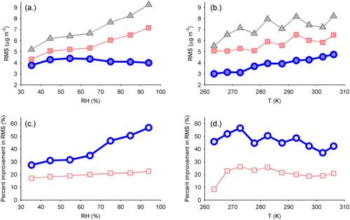
An additional point that we show in Figure 4 is the comparison of our MLR correction model with the simple linear regression correction model available on the Purple Air website and labeled as “University of Utah.” The so-called UUtah correction (as of August 2018 on the Purple Air Website; see Figure S11) is $\mathrm{PM}{2.5}_{\mathrm{UUtah}}=0.778\mathrm{*}\mathrm{PM}{2.5}_{\mathrm{PA}-\mathrm{II}}+2.65$ so we apply that correction to our data and find that while the simple linear regression does improve the accuracy relative to BAM reference PM2.5 (i.e., RMS) by about 18%, there is a major departure for higher RH values (Figure 4c). Our MLR correction, which incorporates RH and T, decreases RMS by over 50% for RH > 80%, while the UUTah correction decreases RMS by less than 20%. The simple linear regression may be somewhat effective in low RH air spaces, but loses effectiveness in air spaces with moderate to high seasonal RH. This is important in the USA, for example, since essentially the central and eastern USA all experience moderate to high RH for most of the year. Not surprisingly, the simple linear regression produces similar improvements for T and RH (Figure 4c and d), but the effect of RH is much more pronounced in our sample location.

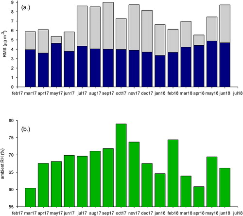
Our data and results also address the question of the reliability of the PA-II IoT sensor package over long deployments with no attempted maintenance. We calculated the monthly averaged RMS values of uncorrected PA-II data and BAM reference data (Figure 2), and corrected PA-II and BAM data (Figure 3) and show this in Figure 5. Initial examination of the RMS for uncorrected PA-II data (Figure 5a) would suggest considerable variability in the performance of the PA-II device with RMS ranging from $5.4-9.0 \text{μg }{\mathrm{m}}^{-3}$ (mean of $7.2\pm 1.3\text{ μg }{\mathrm{m}}^{-3}$). However, after applying the MLR correction that accounts for RH variability (Figure 5b), the RMS ranges from $3.4\text{ to }4.9\mathrm{ }\mu g\mathrm{ }{m}^{-3}$ (mean of $4.1\pm 0.4\text{ μg }{\mathrm{m}}^{-3}$). Thus, for the climatologically humid summer months in North Carolina, our MLR model approach shows that ambient RH variability is accounted for, and that the accuracy of the PA-II device remains nearly constant (within 10%) over a 16-month field deployment and no specific maintenance.

Figure 5. Monthly averaged RMS values calculated relative to reference PM2.5 from BAM using (a) Uncorrected PA-II PM2.5 (gray) and MLR corrected PA-II PM2.5 (dark blue) data, and (b) monthly averaged ambient RH.

Provided a suitable reference PM2.5 dataset is available, either with collocation or with a nearby station, then many of our methods are immediately generalizable to other PA-IIs currently deployed most densely in the USA but also in other locations around the world. The first generalizable finding is that we show that RH and T can and should be accounted for in any linear regression correction (Figure 4). If ambient RH and T are not measured, then the second generalizable finding is that we verified that the RH and T reported by the PA-II device itself is a viable alternative since the offsets relative to ambient RH and T (due to physical design of the PA-II) are linear (Figure S6) and can be directly incorporated in the MLR model (Figure S7) with little loss in accuracy improvements. Third, we also showed that the second particle sensor (“sensor B”) in the PA-II system is an equally viable measurement of PM2.5 (Figure S10).

Noting these choices, we derived MLR fit coefficients for four cases: (1) PA-II particle sensor A using weather station RH and T, (2) PA-II particle sensor B using weather station RH and T, (3) PA-II sensor A using PA-II RH and T, and (4) PA-II sensor B using PA-II RH and T. The MLR fit coefficients for each case are listed in Table 1. The form of the regression model is the same as Equation (1)(1) $$\mathrm{PM}{2.5}_{\mathrm{PA}-\mathrm{II}}=a_0+a_1\mathrm{P}\mathrm{M}{2.5}_{\mathrm{BAM}}+a_2\mathrm{R}\mathrm{H}+a_3\mathrm{T},$$(1) , but each uses different inputs. The first case is the basis for Figure 3, so a comparison of how the correction varies as a function of the input is what we present here.

Table 1. The MLR fit coefficients (Equation (1)(1) $$\mathrm{PM}{2.5}_{\mathrm{PA}-\mathrm{II}}=a_0+a_1\mathrm{P}\mathrm{M}{2.5}_{\mathrm{BAM}}+a_2\mathrm{R}\mathrm{H}+a_3\mathrm{T},$$(1) ) using different predictors and predictands.

MLR predictors	BAM, WxRH, WxT	BAM, WxRH, WxT	BAM, PARH, PAT	BAM, PARH, PAT
MLR predictand	PA-II PM2.5 A	PA-II PM2.5 B	PA-II PM2.5 A	PA-II PM2.5 B
$a_0$	$-25.55\pm 1.87$	$-8.28\pm 1.94$	$-14.20\pm 1.76$	$3.20\pm 1.83$
$a_1$	$1.25\pm 0.01$	$1.34\pm 0.01$	$1.28\pm 0.01$	$1.36\pm 0.01$
$a_2$	$0.099\pm 0.003$	$0.111\pm 0.003$	$0.130\pm 0.004$	$0.142\pm 0.004$
$a_3$	$0.072\pm 0.006$	$0.011\pm 0.007$	$0.032\pm 0.006$	$-0.028\pm 0.006$

Note: For the predictors, “BAM” is the BAM 1022 PM2.5, “WxRH” is the weather station RH, “WxT” is the weather station ambient T, “PARH” is the RH reported by the PA-II, “PAT” is the T reported by the PA-II, “PA-II PM2.5 A” is the PM2.5 reported by sensor A in the PA-II, and “PA-II PM2.5 B” is the PM2.5 reported by sensor B in the PA-II. The $a_0$ coefficient is the constant, while $a_1,$ $a_2,$ and $a_3$ refer to the coefficients associated with the listed predictors.

Figure 6 shows the effect of each of the corrections as a percent difference, difference, and a comparison with the first column (sensor A with weather station data). In row 1, the color scale tends towards cooler colors (blues) when the corrected PM2.5 is less than the uncorrected PM2.5, which is by far the dominant pattern in all corrections due to the high bias relative to the reference PM2.5. Similarly, row 2 has orange-red colors where corrected PM2.5 is greater than uncorrected PM2.5, but for the most part, the corrected PM2.5 is less than uncorrected. Row 3 compares the magnitude of one correction with the correction method in the first column. Warmer colors in this row indicate that the correction method in the first column (using BAM PM2.5, and RH and T from the weather station as predictors of predictand PA-II sensor A PM2.5) reduces the PM2.5 more than the correction in the column itself. Thus, columns 2–4 show that those correction equations reduce uncorrected PM2.5 more than the correction equation in column 1.

Figure 6. The strength of the MLR correction as a function of relative humidity and the input PM2.5. Columns show different correction equations based on (1) PA-II particle sensor A using weather station RH and T, (2) PA-II particle sensor B using weather station RH and T, (3) PA-II sensor A using PA-II RH and T, and (4) PA-II sensor B using PA-II RH and T. Rows (top to bottom) show the percent difference (%) of corrected PM2.5 from uncorrected, the actual difference ($\text{μg }{\mathrm{m}}^{-3}$), and the difference of the correction in the column from the correction in column 1 ($\text{μg }{\mathrm{m}}^{-3}$).

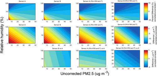
One important result from Figure 6 is how the correction method developed using PM2.5 from sensor A compares with sensor B. In columns 1 and 2 in Figure 6, row 3 shows that result by simply examining the difference in the corrected PM2.5. Recalling that the MLR is based largely on reported (uncorrected) PM2.5 less than $40\text{ μg }{\mathrm{m}}^{-3}$ and RH greater than $40\mathrm{\%},$ the overall difference when using data from the two particle sensors is largely within $3\text{ μg }{\mathrm{m}}^{-3}.$ When using the PA-II RH and T data, columns 3 and 4 show that the magnitude of the correction using sensor A and weather station RH and T is always less by about $0-4\text{ μg }{\mathrm{m}}^{-3}$ which is due mainly to the fact that the PA-II RH is biased low and T is biased high relative to ambient RH and T (Figure S6).

The different MLR corrections together indicate that, to within uncertainty, the reported PA-II PM2.5 can be corrected to be closer to a reference PM2.5. Broad applicability of the values in Table 1 remains to be tested in other regions and may vary due to difference in the dominant chemical composition of the particles (Malm et al. 2004). Varying chemical composition could change the physical and optical properties of the particles as well as the hygroscopicity (Zamora et al. 2019), but it is unclear what the overall effect would be on the corrections discussed in this study. The most direct application of our results would be for PA-II sensors in regions similar to ours, but evaluating the consistency of the correction with other collocation studies will be the best way to understand the broader implications. The methods in our study, however, should be adaptable to any collocation or quasi-collocation study.

5. Conclusions

The PA-II IoT network has provided a massive dataset for air quality scientists and stakeholder communities, and offers a way to understand the microscale within any air space, urban or otherwise. While the accuracy of the IoT devices is less than a maintained FEM device such as the BAM 1022, our correction method shows that hourly corrected PM2.5 data from the PA-II is accurate to within $3-4\text{ μg }{\mathrm{m}}^{-3}$ and suggests that IoT technology is indeed paving a path towards a transformational dataset that would compliment (but not replace) the existing regulatory monitoring network (Kumar et al. 2015; Morawska et al. 2018; Snyder et al. 2013). Our study is limited to hourly PM2.5 less than about $40-50\text{ μg }{\mathrm{m}}^{-3},$ so a key scientific and stakeholder advance would be a dedicated multi-season PA-II or IoT collocation in a polluted air space. This would help understand any potential nonlinearities in the bias between reference PM2.5 and PA-II at higher PM2.5 concentrations. Developing IoT technology for monitoring gaseous pollutants and/or ultrafine particle counts is currently beyond IoT capabilities, but would be a key engineering-based advance that would certainly increase the utility of IoT for a broad range of communities provided a detailed multi-season collocation study is undertaken.

Acknowledgments

We thank Patrick Jones, cartographer in the UNC Charlotte Department of Geography and Earth Sciences, for making the map figure, and Boris Reiss for many valuable discussions during the drafting of the manuscript. We thank Purple Air for maintaining and managing the PA-II data influx and repository.

Additional information

Funding

UNC Charlotte Department of Geography and Earth Sciences provided funding to support the purchase of PA-II sensors for testing. This research did not receive any specific grant from funding agencies in the public, commercial, or not-for-profit sectors.

References

- Berger, R. E., R. Ramaswami, C. G. Solomon, and J. M. Drazen. 2017. Air pollution still kills. New Engl. J. Med. 376 (26):2591–2592. doi:10.1056/NEJMe1706865.
- Carvlin, G. N., H. Lugo, L. Olmedo, E. Bejarano, A. Wilkie, D. Meltzer, M. Wong, G. King, A. Northcross, M. Jerrett, P. B. English, D. Hammond, and E. Seto. 2017. Development and field validation of a community-engaged particulate matter air quality monitoring network in imperial, California, USA. J. Air Waste Manage. Assoc. 67:1342–1352. doi:10.1080/10962247.2017.1369471.
- Castell, N., F. R. Dauge, P. Schneider, M. Vogt, U. Lerner, B. Fishbain, D. Broday, and A. Bartonova. 2017. Can commercial low-cost sensor platforms contribute to air quality monitoring and exposure estimates?. Environ. Int. 99:293–302. doi:10.1016/j.envint.2016.12.007.
- Crilley, L. R., M. Shaw, R. Pound, L. J. Kramer, R. Price, S. Young, A. C. Lewis, and F. D. Pope. 2018. Evaluation of a low-cost optical particle counter (alphasense opc-n2) for ambient air monitoring. Atmos. Meas. Tech. 11 (2):709–720. doi:10.5194/amt-11-709-2018.
- Ebenstein, A., M. Fan, M. Greenstone, G. He, and M. Zhou. 2017. New evidence on the impact of sustained exposure to air pollution on life expectancy from China’s Huai river policy. proc. nat. Academy Sciences 114 (39):10384–10389. doi:10.1073/pnas.1616784114.
- Gao, S., D. A. Hegg, P. V. Hobbs, T. W. Kirchstetter, B. I. Magi, and M. Sadilek. 2003. Water-soluble organic components in aerosols associated with savanna fires in Southern Africa: Identification, evolution, and distribution. J. Geophys. Res. Atmos. 108:8491. doi:10.1029/2002jd002324.
- Gobeli, D., H. Schloesser, and T. Pottberg. 2008. Met one instruments BAM-1020 beta attenuation mass monitor US-EPA PM2.5 federal equivalent method field test results, The Air & Waste Management Association (A&WMA) Conference, Kansas City, MO, January: Citeseer.
- Harrison, R. M. 2018. Urban atmospheric chemistry: A very special case for study. npj Clim. Atmos. Sci. 1:5. doi:10.1038/s41612-017-0010-8.
- Hegg, D. A., and Y. J. Kaufman. 1998. Measurements of the relationship between submicron aerosol number and volume concentration. J. Geophys. Res. Atmos. 103 (D5):5671–5678. doi:10.1029/97JD03652.
- Hegg, D. A., T. Larson, and P.-F. Yuen. 1993. A theoretical study of the effect of relative humidity on light scattering by tropospheric aerosols. J. Geophys. Res. Atmos. 98 (D10):18435–18439. doi:10.1029/93JD01928.
- Hegg, D. A., J. Livingston, P. V. Hobbs, T. Novakov, and P. Russell. 1997. Chemical apportionment of aerosol column optical depth off the mid‐Atlantic Coast of the United States. J. Geophys. Res. Atmos. 102 (D21):25293–25303. doi:10.1029/97JD02293.
- Hoek, G., R. M. Krishnan, R. Beelen, A. Peters, B. Ostro, B. Brunekreef, and J. D. Kaufman. 2013. Long-term air pollution exposure and cardio-respiratory mortality: A review. Environ. Health 12:43. doi:10.1186/1476-069x-12-43.
- Holstius, D. M., A. Pillarisetti, K. R. Smith, and E. Seto. 2014. Field calibrations of a low-cost aerosol sensor at a regulatory monitoring site in California. Atmos. Meas. Tech. 7 (4):1121–1131. doi:10.5194/amt-7-1121-2014.
- Kaufman, A., R. Williams, T. Barzyk, M. Greenberg, M. O'Shea, P. Sheridan, A. Hoang, C. Ash, A. Teitz, M. Mustafa, and S. Garvey. 2017. A citizen science and government collaboration: Developing tools to facilitate community air monitoring. Environ. Justice 10 (2):51–61. doi:10.1089/env.2016.0044.
- Kelly, K. E., J. Whitaker, A. Petty, C. Widmer, A. Dybwad, D. Sleeth, R. Martin, and A. Butterfield. 2017. Ambient and laboratory evaluation of a low-cost particulate matter sensor. Environ. Pollut. 221:491–500. doi:10.1016/j.envpol.2016.12.039.
- Koehler, K. A., S. M. Kreidenweis, P. J. DeMott, A. J. Prenni, C. M. Carrico, B. Ervens, and G. Feingold. 2006. Water activity and activation diameters from hygroscopicity data - part ii: Application to organic species. Atmos. Chem. Phys. 6 (3):795–809. doi:10.5194/acp-6-795-2006.
- Kotchenruther, R. A., and P. V. Hobbs. 1998. Humidification factors of aerosols from biomass burning in Brazil. J. Geophys. Res. Atmos. 103 (D24):32081–32089. doi:10.1029/98JD00340.
- Kreidenweis, S. M., K. Koehler, P. J. DeMott, A. J. Prenni, C. Carrico, and B. Ervens. 2005. Water activity and activation diameters from hygroscopicity data - part i: Theory and application to inorganic salts. Atmos. Chem. Phys. 5 (5):1357–1370. doi:10.5194/acp-5-1357-2005.
- Kumar, P., L. Morawska, W. Birmili, P. Paasonen, M. Hu, M. Kulmala, R. M. Harrison, L. Norford, and R. Britter. 2014. Ultrafine particles in cities. Environ. Int. 66:1–10. doi:10.1016/j.envint.2014.01.013.
- Kumar, P., L. Morawska, C. Martani, G. Biskos, M. Neophytou, S. Di Sabatino, M. Bell, L. Norford, and R. Britter. 2015. The rise of low-cost sensing for managing air pollution in cities. Environ. Int. 75:199–205. doi:10.1016/j.envint.2014.11.019.
- Lewis, A., and P. Edwards. 2016. Validate personal air-pollution sensors. Nature 535 (7610):29–32. doi:10.1038/535029a.
- Lewis, A. C. 2018. The changing face of urban air pollution. Science 359 (6377):744–745. doi:10.1126/science.aar4925.
- Magi, B. I., and P. V. Hobbs. 2003. Effects of humidity on aerosols in Southern Africa during the biomass burning season. J. Geophys. Res. Atmos. 108:8495. doi:10.1029/2002jd002144.
- Magi, B. I., P. V. Hobbs, T. W. Kirchstetter, T. Novakov, D. A. Hegg, S. Gao, J. Redemann, and B. Schmid. 2005. Aerosol properties and chemical apportionment of aerosol optical depth at locations off the U.S. East Coast in July and August 2001. J. Atmos. Sci. 62 (4):919–933. doi:10.1175/JAS3263.1.
- Malm, W. C., B. A. Schichtel, M. L. Pitchford, L. L. Ashbaugh, and R. A. Eldred. 2004. Spatial and monthly trends in speciated fine particle concentration in the United States. J. Geophys. Res. Atmos. 109:D03306. doi:10.1029/2003jd003739.
- McDonald, B. C., J. A. de Gouw, J. B. Gilman, S. H. Jathar, A. Akherati, C. D. Cappa, J. L. Jimenez, J. Lee-Taylor, P. L. Hayes, S. A. McKeen, Y. Y. Cui, S.-W. Kim, D. R. Gentner, G. Isaacman-VanWertz, A. H. Goldstein, R. A. Harley, G. J. Frost, J. M. Roberts, T. B. Ryerson, and M. Trainer. 2018. Volatile chemical products emerging as largest petrochemical source of urban organic emissions. Science 359 (6377):760–764. doi:10.1126/science.aaq0524.
- Morawska, L., P. K. Thai, X. Liu, A. Asumadu-Sakyi, G. Ayoko, A. Bartonova, A. Bedini, F. Chai, B. Christensen, M. Dunbabin, J. Gao, G. S. W. Hagler, R. Jayaratne, P. Kumar, A. K. H. Lau, P. K. K. Louie, M. Mazaheri, Z. Ning, N. Motta, B. Mullins, M. M. Rahman, Z. Ristovski, M. Shafiei, D. Tjondronegoro, D. Westerdahl, and R. Williams. 2018. Applications of low-cost sensing technologies for air quality monitoring and exposure assessment: How far have they gone?. Environ. Int. 116:286–299. doi:10.1016/j.envint.2018.04.018.
- Northcross, A. L., R. J. Edwards, M. A. Johnson, Z.-M. Wang, K. Zhu, T. Allen, and K. R. Smith. 2013. A low-cost particle counter as a realtime fine-particle mass monitor. Environ. Sci. Processes Impacts 15:433–439. doi:10.1039/C2EM30568B.
- Petters, M. D., and S. M. Kreidenweis. 2007. A single parameter representation of hygroscopic growth and cloud condensation nucleus activity. Atmos. Chem. Phys. 7 (8):1961–1971. doi:10.5194/acp-7-1961-2007.
- Posner, L. N., and S. N. Pandis. 2015. Sources of ultrafine particles in the Eastern United States. Atmos. Environ. 111:103–112. doi:10.1016/j.atmosenv.2015.03.033.
- Rai, A. C., P. Kumar, F. Pilla, A. N. Skouloudis, S. Di Sabatino, C. Ratti, A. Yasar, and D. Rickerby. 2017. End-user perspective of low-cost sensors for outdoor air pollution monitoring. Sci. Total Environ. 607:691–705. doi:10.1016/j.scitotenv.2017.06.266.
- Reid, J. S., R. Koppmann, T. F. Eck, and D. P. Eleuterio. 2005. A review of biomass burning emissions part II: Intensive physical properties of biomass burning particles. Atmos. Chem. Phys. 5 (3):799–825. doi:10.5194/acp-5-799-2005.
- Schneider, P., N. Castell, M. Vogt, F. R. Dauge, W. A. Lahoz, and A. Bartonova. 2017. Mapping urban air quality in near real-time using observations from low-cost sensors and model information. Environ. Int. 106:234–247. doi:10.1016/j.envint.2017.05.005.
- Seinfeld, J. H., and S. N. Pandis. 2016. Atmospheric chemistry and physics: From air pollution to climate change. Hoboken, NJ: John Wiley & Sons.
- Sherman, J. P., P. J. Sheridan, J. A. Ogren, E. Andrews, D. Hageman, L. Schmeisser, A. Jefferson, and S. Sharma. 2015. A multi-year study of lower tropospheric aerosol variability and systematic relationships from four North American regions. Atmos. Chem. Phys. 15 (21):12487–12517. doi:10.5194/acp-15-12487-2015.
- Snyder, E. G., T. H. Watkins, P. A. Solomon, E. D. Thoma, R. W. Williams, G. S. W. Hagler, D. Shelow, D. A. Hindin, V. J. Kilaru, and P. W. Preuss. 2013. The changing paradigm of air pollution monitoring. Environ. Sci. Technol. 47:11369–11377. doi:10.1021/es4022602.
- Sousan, S., K. Koehler, L. Hallett, and T. M. Peters. 2016. Evaluation of the alphasense optical particle counter (opc-n2) and the Grimm portable aerosol spectrometer (pas-1.108). Aerosol Sci. Technol. 50 (12):1352–1365. doi:10.1080/02786826.2016.1232859.
- Storksdieck, M., J. Shirk, J. Cappadonna, M. Domroese, C. Göbel, M. Haklay, A. Miller-Rushing, P. Roetman, C. Sbrocchi, and K. Vohland. 2016. Associations for citizen science: Regional knowledge, global collaboration. Citizen Sci. Theory Pract. 1 (2):10. doi:10.5334/cstp.55.
- Wang, Y., J. Li, H. Jing, Q. Zhang, J. Jiang, and P. Biswas. 2015. Laboratory evaluation and calibration of three low-cost particle sensors for particulate matter measurement. Aerosol Sci. Technol. 49 (11):1063–1077. doi:10.1080/02786826.2015.1100710.
- Williams, R., V. Kilaru, E. Snyder, A. Kaufman, T. Dye, A. Rutter, A. Russell, and H. Hafner. 2014. Air sensor guidebook 73. Washington, DC: EPA Office of Research and Development.
- Woodall, G., M. Hoover, R. Williams, K. Benedict, M. Harper, J.-C. Soo, A. Jarabek, M. Stewart, J. Brown, J. Hulla, M. Caudill, A. Clements, A. Kaufman, A. Parker, M. Keating, D. Balshaw, K. Garrahan, L. Burton, S. Batka, V. Limaye, P. Hakkinen, and B. Thompson. 2017. Interpreting mobile and handheld air sensor readings in relation to air quality standards and health effect reference values: Tackling the challenges. Atmosphere 8 (12):182. doi:10.3390/atmos8100182.
- Zamora, M. L., F. Xiong, D. Gentner, B. Kerkez, J. Kohrman-Glaser, and K. Koehler. 2019. Field and laboratory evaluations of the low-cost plantower particulate matter sensor. Environ. Sci. Technol. 53:838–849. doi:10.1021/acs.est.8b05174.