Optimizing the performance of aerosol photoacoustic cells using a finite element model. Part 2: Application to a two-resonator cell

Abstract

Photoacoustic spectroscopy (PAS) measures aerosol absorption in a noncontact manner, providing accurate absorption measurements that are needed to improve aerosol optical property representations in climate models. Central to PAS is resonant amplification of the acoustic pressure wave generated from laser-heated aerosol transferring heat to surrounding gas by a photoacoustic cell. Although this cell amplifies pressure sources from aerosol absorption (signal), it also amplifies noise and background sources. It is important to maximize the cell signal-to-background ratio (SBR) for sensitive absorption measurements. Many researchers have adopted the two-resonator cell design described by Lack et al. (2006). We show that the uncertainty in PAS measurements of aerosol absorption using this two-resonator cell is significantly degraded by its large sensitivity to background contributions from laser scattering and absorption at the cell windows. In Part 1, we described the use of a finite element method (FEM) to predict cell acoustic properties, validated this framework by comparing model predictions to measurements, and used FEM to test various strategies applied commonly to single-resonator cell optimization. In this second part, we apply FEM to understand the excitation of resonant modes of the two-resonator cell, with comparison measurements demonstrating accurate predictions of acoustic response. We perform geometry optimization studies to maximize the SBR and demonstrate that the laser–window interaction background is reduced to undetectable levels for an optimal cell. This optimized two-resonator cell will improve the sensitivity and accuracy of future aerosol absorption measurements.

1. Introduction

The scattering and absorption of light by aerosol particles are important processes occurring in our atmosphere. Indeed, the magnitudes of aerosol–light interactions remain one of the largest uncertainties in climate models (IPCC 2013), with the radiative impact from light-absorbing aerosol constrained poorly in particular (Stier et al. 2007). Large uncertainties in absorption arise from a lack of accurate absorption measurements for atmospheric aerosol and how absorption evolves over particle lifetime and with atmospheric processing (Laskin, Laskin, and Nizkorodov 2015; Moise, Flores, and Rudich 2015; Wang et al. 2018). Reducing these uncertainties requires improved instrumentation for accurate and sensitive measurements of aerosol light-absorption coefficients (α_abs) (Moosmüller, Chakrabarty, and Arnott 2009).

Traditionally, α_abs have been derived from the transmission of light through a filter onto which aerosol is collected, but large uncertainties (of up to 80%) are associated with the derived values of α_abs (Cappa et al. 2008; Lack et al. 2008, 2009), although recent advanced correction schemes show modest biases in derived α_abs values of up to 17% (Davies et al. 2019). These uncertainties arise mostly from the modification of aerosol microphysical properties through interactions with a filter substrate. In recent years, researchers have made significant developments of noncontact techniques for α_abs measurements. Such measurement approaches have included calculation of α_abs from the difference in measured scattering (α_sca) and extinction (α_ext = α_sca + α_abs) coefficients using nephelometry and cavity ring-down spectroscopy, respectively (Strawa et al. 2003). However, this “difference” approach often leads to significant uncertainties in α_abs when α_abs is small. As discussed by Sedlacek and Lee (2007), applying the difference method when α_abs is small involves the subtraction of two quantities with similar magnitudes, with the standard error in the extinction and scattering measurements combining to give significant uncertainty (>60%) in the derived α_abs. Thus, noncontact techniques that probe absorption directly are required. Both photothermal interferometry (Sedlacek 2006; Sedlacek and Lee 2007) and – the focus of this work – photoacoustic spectroscopy (PAS) measure α_abs directly for aerosol in its natural suspended state. These approaches are the techniques-of-choice for accurate, direct, and noncontact measurements of aerosol α_abs.

A full description of PAS is provided in Section 2. Briefly, the consequent periodic pressure wave generated by continuous cycles of laser-induced aerosol heating is measured. This periodic pressure wave results from particles liberating their heat to the bath gas through collisional quenching and the gas undergoing adiabatic cycles of thermal expansion/contraction at a frequency commensurate with the laser modulation frequency. A photoacoustic cell (PA cell) resonantly amplifies the pressure wave for detection by a sensitive microphone, with the amplitude of the microphone response directly proportional to the aerosol absorption coefficient. PAS has been used in laboratory studies to measure α_abs for soot particles (Ajtai et al. 2010; Sharma et al. 2013; Yelverton et al. 2014; Linke et al. 2016) and brown carbon particles produced from the oxidation of toluene organic aerosol in the presence of NO_X (Nakayama et al. 2010). Meanwhile, field studies have included ground-based measurements (Cappa et al. 2008; Bluvshtein et al. 2016) and measurements from aircraft platforms (Arnott et al. 2006; Lack et al. 2012; Davies et al. 2019; Peers et al. 2019). Our research uses a suite of photoacoustic and cavity ring-down spectrometers to measure absorption and extinction coefficients for laboratory-generated aerosol or atmospheric aerosol from aboard research aircraft platforms. By comparing PAS measurements of absorption with that expected from Mie theory, our laboratory measurements (Davies et al. 2018) have demonstrated that PAS measures α_abs to an accuracy better than 8% at optical wavelengths of 405, 514, and 658 nm, i.e., discrete wavelengths that span the visible spectrum. Moreover, Supplementary Table S1 of Fischer and Smith (2018a) shows that PAS measurements of aerosol absorption often achieve sensitivities <1 Mm⁻¹.

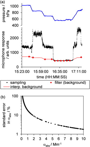
A key consideration of any photoacoustic instrument is the design of the PA cell for the amplification of the periodic photoacoustic pressure wave. The cell is a resonance chamber, where induced pressure waves couple to the resonant mode of the cell when the frequencies are matched. A typical PA cell consists of one or two cylindrical resonators capped by acoustic buffer volumes. While many studies have used single-resonator cells of various sizes (Nakayama et al. 2015; Radney and Zangmeister 2015; Linke et al. 2016; Yu et al. 2017), recent field and laboratory measurements by a growing number of research groups (Lack et al. 2012; Zhang et al. 2016; Bluvshtein et al. 2017; Davies et al. 2018; Fischer and Smith 2018a, 2018b; Cotterell et al. 2019a; Davies et al. 2019; Foster et al. 2019; Peers et al. 2019) have used a two-resonator cell with the same geometry as described in Lack et al. (2006). This two-resonator cell contains a microphone in each resonator, with the microphone signals passed to a differential amplifier to subtract in-phase components of the signals. The uncertainties in PAS measurements of α_abs for spectrometers using this two-resonator cell were assessed by Lack et al. (2012) from both laboratory and aircraft-based studies. The sensitivity in α_abs was determined to lie in the range 0.5–1.5 Mm⁻¹, with an accuracy of ∼10% for α_abs measurements performed from an aircraft platform. Similarly, we have performed our own uncertainty analysis for PAS-measured α_abs (using the two-resonator cell design of Lack et al.) during measurements aboard the UK research aircraft (FAAM BAe-146). Figure 1a shows typical flight data, showing the variation in raw microphone response during a series of straight and level aircraft runs performed at altitudes in the pressure range 550–1000 hPa. The large observed microphone response at pressures above 650 hPa was associated with the aircraft entering an aerosol layer. The plot also shows measurements of the background microphone response at discrete moments in time when filtered air, devoid of any light-absorbing sample, was drawn through the PA cell. There is always a significant background contribution to the raw microphone response. Moreover, this background depends strongly on pressure; the background microphone response is lower at reduced pressure. This background arises almost entirely from the laser beam interacting with the PA cell windows through light scattering (where photon momentum is transferred to the window surface causing mechanical vibrations) and absorption (with light heating the window and generating an additional photoacoustic source). In processing the raw microphone data to calculate α_abs, the background is subtracted. Because the background response cannot be measured at all times, the data analysis relies on a pressure-dependent interpolation to achieve this background subtraction. Figure 1a shows this interpolated background, using the fit of a quadratic polynomial to the measured pressure variation in the background. Uncertainty in the background interpolation degrades the accuracy in the derived aerosol absorption; Figure 1b shows the percentage error in α_abs associated with the uncertainty in the background interpolation with variation in the aerosol absorption amplitude. The standard error in α_abs can be as high as 10–20% for α_abs in the range 1–5 Mm⁻¹, i.e., for typical levels of aerosol absorption. Clearly, removing the dominant background associated with laser–window interactions would considerably reduce the uncertainty and improve the sensitivity in α_abs measurements using the two-resonator cell. Therefore, the cell should amplify the aerosol absorption response (signal) and suppress, or indeed remove, the detection of laser–window interactions (background); any cell optimization study should aim to maximize the signal-to-background ratio (SBR).

Figure 1. (a) Example data for PAS microphone response, using the PA cell design of Lack et al. (2006), over time during airborne measurements aboard the UK research aircraft (FAAM BAe-146), including measurements for sampling ambient aerosol particles and for where the sample was passed through a HEPA filter (background). Measurements were made above the South East Atlantic Ocean during flight C043 of the CLARIFY-2017 field campaign based at Ascension Island (Zuidema et al. 2016). For comparison, we show the variation in pressure associated with changes in altitude over the range 0–7.5 km. The plot also shows the interpolated pressure-dependent background, using a quadratic polynomial to relate the background response to pressure. (b) The standard error in PAS-measured α_abs associated with uncertainty in the interpolated background microphone response.

The design for the current two-resonator cell design was not based on acoustic modeling. Instead, Lack et al. (2006) were inspired by the cell design of Krämer, Bozoki, and Niessner (2001), using two resonators that each contained a microphone. A differential amplifier subtracted the two microphone signals and the authors envisaged that in-phase noise would be removed from the measured response. As shown above, this differential operation does not remove the window background in the Lack et al. cell design; as we will demonstrate, the responses in the two resonators are coupled strongly. Importantly, no study has attempted to optimize the two-resonator cell, despite its widespread adoption by other research groups. In the companion paper (Part 1), we described a finite element method (FEM) framework for predicting the acoustic performance of PA cells. We then validated this framework by comparing model predictions of acoustic properties to measurements for a single-resonator multipass PA cell, the generic structure often used in aerosol cells. We then used this model framework to assess the effectiveness of a range of strategies applied commonly to the optimization of photoacoustic sensitivity for single-resonator cells. In this second part, we apply FEM to the analysis of the two-resonator cell that has recently gained widespread use in leading aerosol absorption measurement research, and optimize its performance to completely suppress the detection of laser–window interactions. Section 2 describes the principles of PAS and the resonant excitation of PA cell modes. Section 3 describes the FEM model used to describe sample and window heating for our two-resonator cell, and describes our measurement cells that were used in validating our model predictions. Section 4 presents an analysis of the acoustic behavior of the existing two-resonator cell before performing optimization studies to design a cell that is insensitive to laser–window interactions.

2. Principles of photoacoustic spectroscopy

The PA process has been described in detail by Rosencwaig (1980), Miklós, Hess, and Bozóki (2001) and in our companion paper (Cotterell et al. 2019b). Intensity-modulated laser light is absorbed by a sample through excitation of molecular rotational, vibrational, and/or electronic energy levels. If the fate of excited molecules is dominated by collisional relaxation (and radiative relaxation, photo-dissociation, and latent heat energy pathways can be ignored), energy is transferred to translational degrees of freedom of the bath gas. This heat transfer causes thermal expansion and generates a pressure wave; the magnitude of this pressure wave is proportional to α_abs. Central to the PA process is the amplification of the pressure wave through excitation of an acoustic eigenmode (standing wave) associated with the geometry of the PA cell. In resonant PAS, the laser power is modulated periodically at the resonance frequency (eigenfrequency) corresponding to the cell eigenmode. Repeated cycles of bath gas thermal expansion/contraction generate a periodic pressure wave that couples efficiently into the cell eigenmode, providing there is sufficient spatial overlap of the eigenmode pressure p_n($\overrightarrow{\mathrm{r}}$) and the heat deposition H($\overrightarrow{\mathrm{r}}$) distributions (see later). The eigenmode has an associated quality factor (Q) describing the energy stored in the resonator relative to the energy lost over one complete period. Often, Q is greater than 50 (Lack et al. 2012; Davies et al. 2018), amplifying the amplitude of the photoacoustic pressure wave by the same factor for subsequent detection by a sensitive microphone located within the cell. Typically, the detected pressure response is on the order of ∼10 µPa and is linearly proportional to α_abs(Bijnen, Reuss, and Harren 1996; Lack et al. 2006, 2012). By calibrating the PAS with a species of known absorption (typically a gaseous absorber, the absorption for which is verified using an independent calibration-free technique such as cavity ring-down spectroscopy), α_abs is determined from the microphone response.

To understand the excitation of modes of an acoustic cavity (i.e., our PA cell), it is useful to consider the general solution to the time-independent wave equation. In the limit of adiabatic compression/expansion during acoustic compression/expansion cycles for an ideal gas, the acoustic pressure distribution p($\overrightarrow{r}$) is found by solving the inhomogeneous wave equation. We write the general solution to this equation as a sum of excitations of resonant eigenmodes $p_n\left(\overrightarrow{r}\right)$ of the cell. These eigenmodes are orthogonal and have associated resonance frequencies $f_n$. Thus, we write the frequency-dependence in the pressure at the microphone location $p\left({\overrightarrow{r}}_M,\omega \right)$ as a sum over eigenmode excitations: (1) $$p\left({\overrightarrow{r}}_M,\omega \right)=\sum _n\frac{i\omega \left(\sigma -1\right)I_0}{\left({\omega }_n^2-{\omega }^2+i\frac{\omega {\omega }_n}{Q_n}\right)}\frac{\int g\left(\overrightarrow{r}\right){\alpha }_{\mathit{abs}}\left(\overrightarrow{r}\right)p_n\left(\overrightarrow{r}\right)dV}{V}{p}_n\left({\overrightarrow{r}}_M\right)$$(1) in which $p_n\left({\overrightarrow{r}}_M\right)$ is the eigenmode pressure at the microphone position, $\omega$ is the angular frequency of the periodically modulated heat (laser intensity) source, ${\omega }_n$ is the resonance angular frequency (${\omega }_n=2\pi f_n$), and Q_n is the quality factor associated with energy losses through thermal and viscous damping processes. A low Q_n corresponds to high levels of thermal and viscous damping. Other important terms are the adiabatic coefficient ($\sigma$), the laser intensity amplitude ($I_0$), the laser intensity spatial distribution ($g\left(\overrightarrow{r}\right)$, e.g., a Gaussian), and the cell volume (V).

The microphone response is given by the absolute value of $p\left({\overrightarrow{r}}_M\right)$ which, for the efficient excitation of a single eigenmode, is given by: (2) $$\left|p\left({\overrightarrow{r}}_M,\omega \right)\right|=\left(\sigma -1\right)I_0{p}_n\left({\overrightarrow{r}}_M\right)\frac{J_n}{V}\sqrt{\frac{Q_n^2/{\omega }_n^2}{1+Q_n^2{\left(\frac{{\omega }_n}{\omega }-\frac{\omega }{{\omega }_n}\right)}^2}}$$(2)

Here, we have defined the overlap integral $J_n=\int g\left(\overrightarrow{r}\right){\alpha }_{\mathit{abs}}\left(\overrightarrow{r}\right)p_n\left(\overrightarrow{r}\right)dV$. This overlap integral for the spatial distributions in the laser power, light-absorbing sample, and pressure eigenmode impacts strongly on the excitation amplitude of a cell resonance. We can assume the absorbing sample occupies the cell homogeneously and the overlap integral is written as $J_n={\alpha }_{\mathit{abs}}\int g\left(\overrightarrow{r}\right)p_n\left(\overrightarrow{r}\right)dV$. Thus, we can describe the frequency-dependent microphone response as a function of the form: (3) $$\left|p\left({\overrightarrow{r}}_M,\omega \right)\right|=p_0\sqrt{\frac{1}{1+Q_n^2{\left(\frac{{\omega }_n}{\omega }-\frac{\omega }{{\omega }_n}\right)}^2}}$$(3)

The general expressions of Equations (1)(1) $$p\left({\overrightarrow{r}}_M,\omega \right)=\sum _n\frac{i\omega \left(\sigma -1\right)I_0}{\left({\omega }_n^2-{\omega }^2+i\frac{\omega {\omega }_n}{Q_n}\right)}\frac{\int g\left(\overrightarrow{r}\right){\alpha }_{\mathit{abs}}\left(\overrightarrow{r}\right)p_n\left(\overrightarrow{r}\right)dV}{V}{p}_n\left({\overrightarrow{r}}_M\right)$$(1) and (2)(2) $$\left|p\left({\overrightarrow{r}}_M,\omega \right)\right|=\left(\sigma -1\right)I_0{p}_n\left({\overrightarrow{r}}_M\right)\frac{J_n}{V}\sqrt{\frac{Q_n^2/{\omega }_n^2}{1+Q_n^2{\left(\frac{{\omega }_n}{\omega }-\frac{\omega }{{\omega }_n}\right)}^2}}$$(2) are useful in describing the manifestation of resonant mode excitation, the functional form of the frequency-dependent microphone response, and the role of the overlap integral in determining mode excitation amplitudes. However, we require quantitative calculations of eigenmode pressure distributions $p_n\left(\overrightarrow{r}\right)$ to predict the microphone response for a given cell geometry. This requires numerical methods such as FEM.

3. Experimental and numerical methods

3.1. A finite element model to predict the acoustic behavior of a two-resonator PA cell

We used FEM to predict the eigenmode pressure distributions $p_n\left(\overrightarrow{r}\right)$ and frequency-dependent microphone response $\left|p\left({\overrightarrow{r}}_M,\omega \right)\right|$ for our two-resonator PA cell and optimize the cell geometry to maximize the SBR. This section provides a brief overview of FEM for predicting PA cell acoustic properties before describing the specific model used to represent our two-resonator cell; the reader is directed to our companion publication for complete details of the principles of using FEM to predict photoacoustic phenomena (Cotterell et al. 2019b).

The amplification of ∼ kilohertz frequency acoustic waves by a photoacoustic cell is a thermo-viscous acoustic process. We are required to solve a set of four equations to predict thermo-viscous acoustic phenomena that involve the perturbations of the three properties of pressure, temperature, and velocity. This set of equations includes the momentum equation, continuity equation, Fourier heat law, and an equation of state. Forming an analytical solution that satisfies these equations is not possible for most geometries and instead we use numerical methods to solve the pressure, temperature, and velocity fields. In FEM, we divide our geometry into many small elements using a mesh of tetrahedral elements. The thermo-viscous acoustic equations are solved numerically for each mesh element, with the solutions for adjacent elements coupled by boundary conditions. Importantly, the internal surfaces of the PA cell contribute to damping of acoustic energy through thermal and viscous damping. Thermal damping arises from the isothermal heat transfer between the high thermal conductivity surfaces of typical metal cells and the closest layer of air. Viscous damping arises from the no-slip boundary condition that requires the tangential velocity be zero for molecules closest to the cell surfaces. As we show in our companion paper for a 1500-Hz acoustic wave in air, thermal and viscous energy losses occur over boundary layer thicknesses of ∼70 µm and ∼60 µm, respectively (Cotterell et al. 2019b). These thermal and viscous boundary layer losses are the dominant contributors to damping and thus lead to the reduction of Q factors for resonant modes.

To calculate eigenmode pressure distributions and frequency-dependent microphone responses, we used the thermoviscous acoustics interface in the FEM modeling software COMSOL Multiphysics 5.2a (COMSOL Group, Stockholm, Sweden). We investigated the performance of our two-resonator cell for the cases of using either flat or Brewster-angled windows. While our measurements have exploited Brewster-angled windows to minimize scattering of incident laser light (Davies et al. 2018; Cotterell et al. 2019a), researchers using the same cell design have used flat windows (Lack et al. 2012; Bluvshtein et al. 2017; Fischer and Smith 2018b; Foster et al. 2019). Figures 2a and b show the respective meshed geometries for the flat and Brewster-angled window cells; the Brewster window cell mimics the flat window cell, albeit having additional Brewster-angled volumes. Moreover, Figure 2c labels the parameters that describe completely the cell geometries, and Table 1 provides values for these parameters that describe the cells used in our own measurements and in studies by other researchers. The cells consist of two parallel and cylindrical resonators (an upper and lower resonator), each of length l_res and radius r_res, that are separated by a center-to-center distance d_res and connected by capping buffer volumes affixed to each resonator end. These buffer volumes are characterized by a length l_buf, height h_buf, width w_buf, and a fillet radius r_fil. Each buffer volume is affixed to a cylindrical volume (referred to as window volumes) onto which windows are affixed. The window volumes have a length l_win and radius r_win. We applied two mirror symmetry boundaries to reduce computational cost, with these two mirror planes indicated in Figure 2a. Specifically, there is mirror symmetry in the z-x plane (longitudinal mirror plane) and in the z-y plane (transverse mirror plane). All domains are solved for in the COMSOL Multiphysics thermoacoustics frequency domain interface with equilibrium temperature and pressure set to T₀ = 293.15 K and p₀ = 101,325 Pa (one atmosphere). All the required thermodynamic properties of air (e.g., viscosity, equilibrium density, heat capacity, and thermal conductivity) are taken from the COMSOL Multiphysics material library. We assigned no-slip and isothermal boundary conditions to all surfaces of the cell.

Figure 2. (a) The meshed geometry for the two-resonator cell with flat windows including two reflection symmetry planes; one parallel to the z-x plane through the center of the cell (longitudinal mirror plane) and one parallel to the z-y plane (transverse mirror plane). (b) The meshed geometry for the Brewster window cell. (c) Labeled dimensions for the Brewster window cell, with perspectives along the longitudinal and transverse mirror planes. Table 1 provides values for these dimensions. (d) For the Brewster window cell, the highlighted volumes indicate regions where periodic sample or window heating was applied.

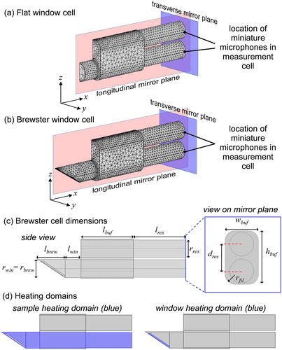
Table 1. Geometric parameters for the two-resonator PA cell.

Quantity	Description	Value
lres	Length of resonators	11.0 cm
rres	Radius of resonators	1.0 cm
dres	Separation of the lower and upper resonator centers	2.2 cm
lbuf	Length of buffer volumes	5.5 cm (lres/2)
hbuf	Height of buffer volumes	4.2 cm
wbuf	Width of buffer volumes	2.6 cm
rfil	Fillet radius for corners of buffer volumes	0.8 cm
lwin	Length of window volumes	1.0 cm
rwin	Radius of window volumes	1.0 cm
θB	Brewster angle for UV fused silica at optical wavelength of 660 nm	55°

An important consideration in any FEM model is the division of the geometry into mesh elements; FEM calculations are computationally expensive if the mesh is very fine, while a coarse mesh will fail to capture important physical processes. Figures 2a and b show the PA cell models including the finite element mesh. The mesh consisted of a bulk and boundary layer mesh, with the latter mesh of a higher spatial resolution to resolve thermal and viscous damping at the air–surface interface. The bulk mesh had a maximum and minimum tetrahedral element size of 5.72 mm (corresponding to ∼1/40 of the acoustic wavelength) and 1.15 mm (∼1/200 of the acoustic wavelength), respectively. Other relevant bulk mesh parameters include the maximum element growth rate, curvature factor, and resolution of narrow regions, which were set to 1.5, 0.3, and 0.7, respectively. For the boundary layer mesh, the maximum layer decrement was set to 300, with 10 layers resolving a total boundary layer mesh thickness of 100.6 µm. Our model ignores some aspects of our measurement cell that would prevent mirror symmetry planes being used and lead to long calculation times, including a humidity probe that is inserted into the cell during measurements, small electret microphones located at each resonator center, a miniature speaker that is located within the lower resonator, and the sample inlet/outlet ports.

In our experimental measurements, a multipass laser beam propagates parallel to the x-axis through the center of the lower resonator. Figure 2d shows the domains that were heated in our Brewster-angled window cell model to represent sample heating. The heat deposited H was represented by: (4) $$H\left(\overrightarrow{r}\right)=I_{0}g\left(\overrightarrow{r}\right){\alpha }_{\mathit{abs}}\left(\overrightarrow{r}\right)=\frac{I_0}{\pi w^2}\exp \left(-\frac{y^2+z^2}{2w^2}\right){\alpha }_{\mathit{abs}}$$(4) with the laser intensity spatial distribution $g\left(\overrightarrow{r}\right)$ described by a Gaussian distribution of beam waist $w$, while y and z represent the transverse distances from the cylindrical axis through the center of the lower resonator. In all simulations of sample heating, we used I₀ = 0.1 W, w = 0.5 mm and a sample absorption coefficient ${\alpha }_{\mathit{abs}}$ = 5 Mm⁻¹, a typical absorption coefficient for atmospheric aerosol (Lack et al. 2012). The important parameter for geometry optimization is the SBR, requiring simulations of microphone responses for both sample heating and laser–window interactions. Figure 2d shows the window-heating domain used in simulating the latter microphone responses in the Brewster cell, with the cylindrical heating domain oriented at the Brewster angle, having a radius 0.9r_win, thickness 2 mm, and located 1 mm from the boundary of the window volume. The window-heating domain for the flat-window cell took similar dimensions, but was oriented such that the incident laser beam propagated normal to the window face. The heat deposited in the window-heating domain was also described by Equation (4)(4) $$H\left(\overrightarrow{r}\right)=I_{0}g\left(\overrightarrow{r}\right){\alpha }_{\mathit{abs}}\left(\overrightarrow{r}\right)=\frac{I_0}{\pi w^2}\exp \left(-\frac{y^2+z^2}{2w^2}\right){\alpha }_{\mathit{abs}}$$(4) using the same parameters above, albeit using the absorption coefficient for N-BK7 glass (https://refractiveindex.info/) at a 550-nm optical wavelength (${\alpha }_{\mathit{abs}}$ = 0.1653 m⁻¹). We did not include any pressure sources to mimic light scattering from the cell windows as this proved not possible in the COMSOL Multiphysics thermos–viscous acoustics interface without perturbing the no-slip and isothermal boundary conditions.

COMSOL Multiphysics was used to simulate the eigenmode pressure distributions p_n($\overrightarrow{r}$) and their associated eigenfrequencies. Furthermore, we modeled the frequency-dependent variation in pressure with acoustic excitation provided by either sample or window heating as described above. In our measurements with a two-resonator cell, small electret microphones were located at the longitudinal center of each resonator with these microphone responses passed through a differential amplifier. Therefore, the quantities of interest from the frequency domain studies are the pressures at the microphone positions for the lower ($p\left({\overrightarrow{r}}_{M,\mathit{low}},\omega \right)$) and upper ($p\left({\overrightarrow{r}}_{M,\mathit{up}},\omega \right)$) resonators. We calculated $p\left({\overrightarrow{r}}_{M,\mathit{low}},\omega \right)$ and $p\left({\overrightarrow{r}}_{M,\mathit{up}},\omega \right)$ from pressure simulations by evaluating the pressure at the surface of a resonator at the position of the transverse (horizontal) mirror plane. These pressures can be positive or negative (relative to a background pressure), depending on phase. We define the differential operation response of the PA cell at a given modulation frequency as: (5) $$p\left({\overrightarrow{\mathrm{r}}}_{\mathrm{M},\mathit{dif}}\right)=p\left({\overrightarrow{\mathrm{r}}}_{\mathrm{M},\mathit{low}}\right)-p\left({\overrightarrow{\mathrm{r}}}_{\mathrm{M},\mathit{up}}\right)$$(5) where we have omitted the angular frequency term for brevity. In addition, we append the superscripts “sig” and “bck” to $p\left({\overrightarrow{\mathrm{r}}}_{\mathrm{M},\mathit{low}}\right)$, $p\left({\overrightarrow{\mathrm{r}}}_{\mathrm{M},\mathit{up}}\right),$ and $p\left({\overrightarrow{\mathrm{r}}}_{\mathrm{M},\mathit{dif}}\right)$ to denote whether excitation was provided by sample (signal) and window (background) heating, respectively. The predicted microphone responses are given by the moduli of these quantities, i.e., $\left|p\left({\overrightarrow{\mathrm{r}}}_{\mathrm{M},\mathit{low}}\right)\right|$, $\left|p\left({\overrightarrow{\mathrm{r}}}_{\mathrm{M},\mathit{up}}\right)\right|$, and $\left|p\left({\overrightarrow{\mathrm{r}}}_{\mathrm{M},\mathit{dif}}\right)\right|$.

3.2. Experimental measurements of photoacoustic cell performance

Our previous publications described our PAS instruments in detail (Davies et al. 2018; Cotterell et al. 2019a) and only a brief overview of our experimental methods is provided here. Our instrument comprised of five photoacoustic spectrometers that sampled from a common inlet, with each spectrometer driven by a separate laser. Two spectrometers operated at an optical wavelength of 405 nm, one at 514 nm and two at 658 nm. Each of the five PA cells used in experimental measurements had the same geometry as that described in the previous section and were machined from aluminum alloy. The temperatures of all cells were controlled and maintained at 293K using thermo-electric controllers. Measurements with flat windows used one-inch diameter N-BK7 windows (Edmund Optics), while measurements with Brewster-angled windows used UV-fused silica Brewster windows (Thorlabs, BW2502). The output from a continuous-wave diode laser was directed into an astigmatic multipass optical cavity that provided multiple reflections (∼50) of the laser beam through the lower resonator of the PA cell. This optical cavity was external to the cell. The intensity of the laser beam was periodically modulated at an angular frequency ω. Inlet and outlet ports were located in opposite acoustic buffer volumes and the sample flow was drawn through the cell. The design of the inlet and outlet pipes were identical to those used in our previous publications (Davies et al. 2018, 2019; Cotterell et al. 2019a; Peers et al. 2019) and consist of 0.25-inch stainless steel tubing connected to an acoustic notch filter (designed to remove acoustic noise from the sample pump) with an inner diameter twice that of the connecting 0.25-inch inlet pipe. The dimensions of the inlet system provide efficient transmission of sub-micron diameter aerosol particles; we measured the aerosol transmission efficiency for a range of mobility-selected diameter aerosols through the inlet pipe, photoacoustic cell, and then the outlet, with transmission losses of <1% measured for sub-micron diameter aerosols. The sensitive microphones located at the longitudinal center of each resonator recorded a voltage that was linearly proportional to the pressure at each microphone location. The voltage from each microphone was passed through a differential amplifier and the amplified output sent to a data acquisition (DAQ) card that recorded the microphone waveform with a time resolution of 8 MSa/s over a one-second interval.

A speaker was located close to the microphone in the lower resonator and was driven by a voltage waveform that, in the frequency domain, was a top-hat distribution over the frequency range 1300–1700 Hz. The speaker could be used to excite a selection of cell eigenmodes. The one-second microphone time trace was recorded and processed through a Fast Fourier Transform that gave an acoustic spectrum. In this way, the resonance mode distributions in the frequency domain were measured; the resonance frequencies f_n and quality factors Q_n were determined by fitting the measured frequency-dependent $\left|p\left({\overrightarrow{\mathrm{r}}}_{\mathrm{M},\mathit{low}}\right)\right|$, $\left|p\left({\overrightarrow{\mathrm{r}}}_{\mathrm{M},\mathit{up}}\right)\right|,$ or $\left|p\left({\overrightarrow{\mathrm{r}}}_{\mathrm{M},\mathit{dif}}\right)\right|$ to Equation (3)(3) $$\left|p\left({\overrightarrow{r}}_M,\omega \right)\right|=p_0\sqrt{\frac{1}{1+Q_n^2{\left(\frac{{\omega }_n}{\omega }-\frac{\omega }{{\omega }_n}\right)}^2}}$$(3) .

To measure the PAS response from sample or window absorption, the microphone response was recorded for one second and processed via a Fast Fourier Transform, and the frequency component of this response corresponding to the laser modulation frequency was measured. This measured photoacoustic signal is referred to as the IA. In measurements of the background photoacoustic signal (IA_bck) from laser–window interactions, the cell was devoid of any light-absorbing sample and filled with zero air passed through a HEPA filter to remove aerosol particles and a NO_X and O₃ scrubber to remove light-absorbing gases.

4. Results and discussion

We used our FEM model to understand the acoustic properties of the two-resonator PA cell. Sections 4.1 and 4.2 assess the performance of the two-resonator cell with flat and Brewster-angled windows, respectively, demonstrating good agreement in acoustic properties between model predictions and measurements. Section 4.3 focusses on the optimization of a comprehensive range of cell dimensions to maximize the SBR. Based on these optimization studies, Section 4.4 examines the performance of an optimized two-resonator cell, compares model predictions with measurements, and demonstrates that the detection of window background is completely suppressed.

4.1. Two-resonator PA cell with flat windows

4.1.1. The supported eigenmodes

We simulated the pressure eigenmodes p_n($\overrightarrow{r}$) supported by the cell. We note that the model cannot identify eigenmodes that are antisymmetric about the mirror symmetry planes. Section S1 of the online Supplementary Information (SI) demonstrates the loss of identified eigenmodes with increasing mirror symmetry. In particular, the n = 1 mode (f₁ ≈ 600 Hz) has antisymmetric symmetry about the transverse mirror plane and is not located when this mirror symmetry is applied. However, this mode has pressure nodes at the microphone locations, and its excitation is not detectable. Moreover, this mode is not excited by a heat distribution g($\overrightarrow{\mathrm{r}})$ source that is symmetric about the transverse mirror plane as the overlap integral J₁ evaluates to zero. For these reasons, and that the n = 1 mode is well separated from other modes by >500 Hz, we ignore the n = 1 mode in our analysis.

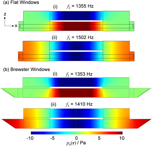
Figure 3a shows the p_n($\overrightarrow{r}$) for the n = 2, 3 eigenmodes of the flat window cell. The n = 2 mode is a “ring” mode, with the standing wave having antinodes (pressure extremum) in each resonator of opposite phase, while a pressure node is found close to the cell windows. In the time domain, the n = 2 pressure oscillates with the extremum in each resonator varying in phase from –π to +π at a periodic frequency of f₂ = 1355 Hz. The n = 3 mode is a longitudinal mode with pressure antinodes at the window boundaries in addition to antinodes at the resonator centers. The resonance frequency of the n = 3 mode is f₃ = 1502 Hz and is separated from the f₂ resonance frequency by ∼150 Hz. We refer to the n = 2 and n = 3 mode as the ring and longitudinal modes, respectively. It is useful to consider the physical processes that lead to the formation of the ring and longitudinal modes.

Figure 3. Comparison of the eigenmode pressure distributions for the two-resonator cell with either (a) flat windows or (b) Brewster-angled windows.

The pressure distributions of the longitudinal and ring mode are the in-phase and out-of-phase conditions for two strongly coupled open Fabry–Pérot (FP) resonators (Ward et al. 2016). In the absence of the capping buffer volumes (i.e., for a resonator opening into an infinite volume), the eigenmode of each resonator requires pressure nodes (x component of velocity field are antinodes) at its ends and an integer number of half-wavelengths supported over its length. To first order, the frequencies of the FP modes are given by f_FP,q = qc/2l_res, with c the speed of sound (343 ms⁻¹ at room temperature and pressure) and q the FP mode order. In this way, we can predict the first (q = 1) FP mode to have an eigenfrequency of 1556 Hz for l_res = 11 cm, similar to the FEM prediction for the longitudinal mode. However, in this calculation, we have neglected the end correction associated with evanescent wave diffraction, and it is these evanescent fields that determine whether the individual cavities are coupled to give the longitudinal (in-phase) or ring (out-of-phase) mode. We direct the reader to Ward et al. 2016 for a thorough discussion of the types of acoustic modes arising in close-lying resonator pipes, including those corresponding to the ring and longitudinal modes. We stress that the formation of the ring mode in the two-resonator PA cell is unique to cells containing multiple resonators and is clearly not formed in a single-resonator PA cell.

4.1.2. Mode excitation through sample heating

We investigated the PA cell response to sample or window heating excitation, simulating the microphone responses with variation in the laser modulation frequency over the frequency range of 1300–1600 Hz. For sample heating, Figure 4a shows the predicted frequency-dependent responses for $\left|p^{\mathit{sig}}\left({\overrightarrow{\mathrm{r}}}_{\mathrm{M},\mathit{low}}\right)\right|$, $\left|p^{\mathit{sig}}\left({\overrightarrow{\mathrm{r}}}_{\mathrm{M},\mathit{up}}\right)\right|,$ and $\left|p^{\mathit{sig}}\left({\overrightarrow{\mathrm{r}}}_{\mathrm{M},\mathit{dif}}\right)\right|$ at frequencies close to the ring mode eigenfrequency f₂ = 1355 Hz. The microphone pressures at the longitudinal mode eigenfrequency (f₃ = 1502 Hz) were negligible and therefore the responses at frequencies >1400 Hz are not shown. Sample heating excitation at the longitudinal mode eigenfrequency is very weak for two reasons. First, Figure 3a shows that the longitudinal mode has relatively similar portions of positive and negative eigenmode pressure along the length of the laser beam heating volume (see also the line profile in Supplementary Figure S2(a) of the SI). Thus, the overlap integral J₃ in Equation (2)(2) $$\left|p\left({\overrightarrow{r}}_M,\omega \right)\right|=\left(\sigma -1\right)I_0{p}_n\left({\overrightarrow{r}}_M\right)\frac{J_n}{V}\sqrt{\frac{Q_n^2/{\omega }_n^2}{1+Q_n^2{\left(\frac{{\omega }_n}{\omega }-\frac{\omega }{{\omega }_n}\right)}^2}}$$(2) evaluates to near zero. Second, the longitudinal eigenmode pressure at the two resonator centers are similar in magnitude and equal in phase, giving near-perfect subtraction of any microphone-detected excitation of the longitudinal mode for the differential amplified response.

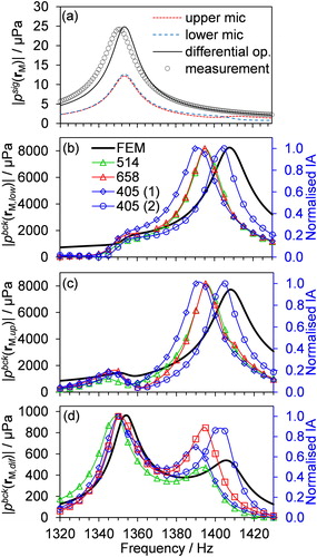
Figure 4. FEM predictions for the flat window cell of the frequency-dependent pressure responses $\left|p\left({\overrightarrow{\mathrm{r}}}_{\mathrm{M},\mathit{low}}\right)\right|$, $\left|p\left({\overrightarrow{\mathrm{r}}}_{\mathrm{M},\mathit{up}}\right)\right|,$ and $\left|p\left({\overrightarrow{\mathrm{r}}}_{\mathrm{M},\mathit{dif}}\right)\right|$ . Simulations are shown for the cases of (a) sample heating (α_sample = 5 Mm⁻¹) and (b) window heating (α_win = 0.1653 m⁻¹). We compare the sample heating simulations to measured data using speaker excitation, with measurements representing the mean response over five PA spectrometers.

Figure 4a shows that there is a significant microphone response at the ring mode eigenfrequency. This large microphone response is due to the nonzero overlap integral J₂; Figure 3a shows that the eigenmode pressure along the path length of the laser beam is always positive (see also the line profile in Supplementary Figure S2(a)). Moreover, Figure 4a shows that the individual microphone pressure responses $\left|p^{\mathit{sig}}\left({\overrightarrow{\mathrm{r}}}_{\mathrm{M},\mathit{low}}\right)\right|$ and $\left|p^{\mathit{sig}}\left({\overrightarrow{\mathrm{r}}}_{\mathrm{M},\mathit{up}}\right)\right|$ are similar in amplitude. However, the phase of the ring mode pressure field at the two microphone locations is opposite and the differential response $\left|p^{\mathit{sig}}\left({\overrightarrow{\mathrm{r}}}_{\mathrm{M},\mathit{dif}}\right)\right|$ is thus amplified. Fitting the frequency dependent $\left|p^{\mathit{sig}}\left({\overrightarrow{\mathrm{r}}}_{\mathrm{M},\mathit{dif}}\right)\right|$ to Equation (3)(3) $$\left|p\left({\overrightarrow{r}}_M,\omega \right)\right|=p_0\sqrt{\frac{1}{1+Q_n^2{\left(\frac{{\omega }_n}{\omega }-\frac{\omega }{{\omega }_n}\right)}^2}}$$(3) gives a best-fit ring mode quality factor of Q₂ = 104.6 ± 2.6.

Figure 4a also shows the mean response measured from the five PA spectrometers in our instrument. In these measurements, speaker excitation was used to measure the resonance mode distributions. For comparison purposes, the measured microphone response is normalized to the 27.1 µPa amplitude of the model prediction for $\left|p^{\mathit{sig}}\left({\overrightarrow{\mathrm{r}}}_{\mathrm{M},\mathit{dif}}\right)\right|$; the microphones were not calibrated, so conversion of the measured voltages to a pressure was not possible. There is good agreement between the predicted and measured distributions, with the measured distribution having f₂ = 1344.6 ± 0.8 Hz and Q₂ = 94.5 ± 2.7. Our model overestimates Q₂ (underestimates thermal and viscous damping) by 10.7%, while f₂ is overestimated by 10 Hz (<1%). The reasons for these discrepancies include that our model does not include a humidity probe that protrudes into a buffer volume of our measurement cell and neglects the impedances introduced by the speaker, microphone, and sample inlet/outlet ports. Moreover, additional thermal and viscous energy dissipation arises from the surfaces of the cell that our model assumes as perfectly smooth.

4.1.3. Mode excitation through window heating

Figure 4b shows the frequency-dependent pressure for the case of acoustic excitation from laser heating of the windows. The frequency responses $\left|p^{\mathit{sig}}\left({\overrightarrow{\mathrm{r}}}_{\mathrm{M},\mathit{low}}\right)\right|$ and $\left|p^{\mathit{sig}}\left({\overrightarrow{\mathrm{r}}}_{\mathrm{M},\mathit{up}}\right)\right|$ are not symmetric about the ring mode eigenfrequency, but a Lorentzian pressure distribution is recovered when the microphone responses are passed through a differential amplifier. The nonsymmetric distributions for the individual microphone responses is explained by accounting for acoustic excitation of both the ring and longitudinal eigenmodes. Section S2 of the SI explains this nonsymmetric response using an empirical model. Crucially, the J_n (i.e., the overlap integral for the pressure, absorber, and laser power distributions; see Section 2) for window heating is ∼60 times larger for the longitudinal compared to the ring mode. Thus, even though the longitudinal and ring eigenfrequencies are separated by 150 Hz, the strong longitudinal mode excitation gives a significant longitudinal mode contribution to the individual microphone responses at the ring mode eigenfrequency. However, the longitudinal mode contribution is almost completely removed by the differential amplifier as the longitudinal mode pressure in the two resonators have near-equal phase. Meanwhile, the ring mode contribution is amplified and a Lorentzian distribution is recovered for $\left|p^{\mathit{sig}}\left({\overrightarrow{\mathrm{r}}}_{\mathrm{M},\mathit{dif}}\right)\right|$.

Taking the ratio of the differential-operation amplitudes $\left|p^{\mathit{sig}}\left({\overrightarrow{\mathrm{r}}}_{\mathrm{M},\mathit{dif}},{\omega }_2\right)\right|$ and $\left|p^{\mathit{bck}}\left({\overrightarrow{\mathrm{r}}}_{\mathrm{M},\mathit{dif}},{\omega }_2\right)\right|$ (differential microphone responses at the ring mode eigenfrequency), SBR = 0.112. This SBR value is useful for comparing to the performance of other cell geometries in later sections. In the discussion above, we have shown that window background sources couple very efficiently into the longitudinal mode compared to the ring mode and the differential amplifier removes most of the longitudinal mode detection. Without differential operation, p₀^sig is 50% lower, while p₀^bck 35% higher and the SBR would be 0.042, a decrease of 63%. Therefore, it is important that researchers using the two-resonator cell design use a differential amplification detection scheme to maximize the sensitivity of their measurements.

4.2. Two-resonator PA cell with Brewster-angled windows

We now assess the performance of the two-resonator cell with Brewster windows and compare this performance with that of the flat window cell.

4.2.1. The supported eigenmodes

Figure 3b shows the eigenmode pressure distributions for the Brewster window cell. The eigenmode pressure distributions are similar to those for the flat window cell, although the longitudinal mode has a lower eigenfrequency for the Brewster window cell. The reduction in n = 3 eigenfrequency is caused by the longer length of the cell upon the inclusion of the Brewster windows, giving a longer acoustic wavelength. Meanwhile, the ring mode eigenfrequency is not sensitive to changes in window dimensions; the pressure field couples between the two resonator pipes and has minimal interaction with the window volumes. The n = 2, 3 eigenfrequencies are separated by only 57 Hz for the Brewster window cell, compared to a ∼150 Hz separation for the flat window cell. This reduced frequency spacing for the Brewster cell has implications for the detection of single-mode excitation.

4.2.2. Mode excitation through sample heating

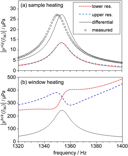
Figure 5a compares the predicted |p^sig(${\overrightarrow{\mathrm{r}}}_{\mathrm{M},\mathit{dif}}$)| with the measured differential amplifier response for speaker excitation, averaged for our five PA cells. For comparison purposes, we have scaled the amplitude of the measured response to equal the amplitude of the model distribution. The measured response has a Lorentzian distribution with f₂ = 1350.6 ± 1.1 Hz and Q = 91.7 ± 3.3. The model predicts f₂ = 1353.4 ± 0.1 Hz, larger than the measured value by 2.8 Hz, and Q = 104.6 ± 0.4, larger than the measured value by 12.9. These discrepancies arise for the same reason outlined in Section 4.1.2; our model ignores the humidity probe that protrudes into our measurement cell and neglects the impedances from the speaker, microphones, and sample inlet/outlet ports. Moreover, the measurement cells were temperature stabilized using a thermo-electric controller and, while we performed both our simulations and experimental measurements for a temperature of 293.15 K, systematic biases in the cell temperature are possible. If the 2.8-Hz discrepancy in f₂ between model and measurement were caused exclusively by a systematic error in temperature, the temperature bias would have to be 1.3 K, with experimental biases in temperature of ∼1 K possible. In particular, our temperature control uses a thermistor embedded within the wall of the aluminum-alloy cell, and the internal air temperature was not measured directly.

Figure 5. FEM predictions of microphone response for the Brewster window cell compared with measured data. (a) Simulations of $\left|p^{\mathit{sig}}\left({\overrightarrow{\mathrm{r}}}_{\mathrm{M}},\omega \right)\right|$ for the individual microphone and differential responses compared to measured differential operation data using speaker excitation. (b),(c),(d) Predictions of $\left|p^{\mathit{bck}}\left({\overrightarrow{\mathrm{r}}}_{\mathrm{M}},\omega \right)\right|$ (window heating) with the measured IA_bck for detection by the lower microphone, upper microphone, and differential response, respectively. Measured data are shown for four separate PA spectrometers using 405 nm (two spectrometers), 514 nm, or 658 nm laser excitation. The measured IA_bck has been normalized to scale from 0 to 1. The lines for the measured IA series are to guide the eye only.

4.2.3. Mode excitation through window heating

Figures 5b–d show predictions of |p^bck(${\overrightarrow{\mathrm{r}}}_{\mathrm{M},\mathit{low}}$)|, |p^bck(${\overrightarrow{\mathrm{r}}}_{\mathrm{M},\mathit{up}}$)|, and |p^bck(${\overrightarrow{\mathrm{r}}}_{\mathrm{M},\mathit{dif}}$)|, respectively, compared with measurements using our spectrometers with either 405, 514, or 658 nm laser excitation. Measurements using our second 658-nm PA spectrometer are not shown due to a faulty laser at the time of measurement. There is good agreement between model predictions and measurements for both individual microphone and differential responses. For the individual microphone responses, the simulations agree well with the measured response, even showing subtle features such as the contribution of ring mode excitation in the 1340–1360 Hz range. For |p^bck(${\overrightarrow{\mathrm{r}}}_{\mathrm{M},\mathit{dif}}$)|, the ring mode excitation is amplified while the longitudinal mode excitation from the individual microphone responses is partly removed. To rationalize the incomplete removal of longitudinal mode detection in the differential response, Supplementary Figure S3 shows line profiles through the n = 3 pressure eigenmode distribution for profiles through both the upper and lower resonators. For both Brewster-angled and flat windows, the eigenmode pressure at the microphone position (x = 0) is more negative in the lower compared to the upper resonator. However, the difference in eigenmode pressure between the two microphones is larger for the Brewster window cell compared to that of using flat windows. This larger difference in p_n=3(${\overrightarrow{\mathrm{r}}}_{\mathrm{M}}$) for the Brewster window cell corresponds to a difference in phase, leading to incomplete removal of longitudinal mode detection by the differential amplifier.

Our model agrees well with the window heating measurements in Figure 5 for the ring mode excitation, while the longitudinal mode eigenfrequency is predicted to be slightly larger than the measured values. The average measured longitudinal mode eigenfrequency is 1395.6 ± 5.2 Hz, lower than the predicted value by 14.4 Hz. Even in the measured data for our four PA cells, the n = 3 eigenfrequency varies considerably and cannot be rationalized by variations in cell temperature. We show in Section 4.3.1 that the longitudinal mode eigenfrequency is very sensitive to small variations in the length of the buffer volumes; a 1-mm increase in l_buf is predicted to decrease the longitudinal mode eigenfrequency by 7.7 Hz. Therefore, a + 2 mm error in the buffer lengths could be responsible for the 14-Hz eigenfrequency discrepancy. Meanwhile, discrepancies between measured and predicted longitudinal mode amplitudes are likely caused by small differences in sensitivity for the upper and lower microphones.

We can estimate the contribution of n = 3 mode excitation to detection of window background at the n = 2 eigenfrequency by fitting the predicted |p^bck$({\overrightarrow{\mathrm{r}}}_{\mathrm{M},\mathit{dif}},\omega )$| to a bimodal distribution consistent with Equation (1)(1) $$p\left({\overrightarrow{r}}_M,\omega \right)=\sum _n\frac{i\omega \left(\sigma -1\right)I_0}{\left({\omega }_n^2-{\omega }^2+i\frac{\omega {\omega }_n}{Q_n}\right)}\frac{\int g\left(\overrightarrow{r}\right){\alpha }_{\mathit{abs}}\left(\overrightarrow{r}\right)p_n\left(\overrightarrow{r}\right)dV}{V}{p}_n\left({\overrightarrow{r}}_M\right)$$(1) : (6) $$\left|p\left({\overrightarrow{r}}_M,\omega \right)\right|=A_2\sqrt{\frac{1}{1+Q_2^2{\left(\frac{f_2}{f}-\frac{f}{f_2}\right)}^2}}+A_3\sqrt{\frac{1}{1+Q_3^2{\left(\frac{f_3}{f}-\frac{f}{f_3}\right)}^2}}$$(6) in which A_n are the amplitude contributions of the n = 2, 3 modes. We used a least-squares routine that varied A_n, f_n, and Q_n for each mode to fit Equation (6)(6) $$\left|p\left({\overrightarrow{r}}_M,\omega \right)\right|=A_2\sqrt{\frac{1}{1+Q_2^2{\left(\frac{f_2}{f}-\frac{f}{f_2}\right)}^2}}+A_3\sqrt{\frac{1}{1+Q_3^2{\left(\frac{f_3}{f}-\frac{f}{f_3}\right)}^2}}$$(6) to the predicted |p^bck$\left({\overrightarrow{\mathrm{r}}}_{\mathrm{M},\mathit{dif}},\omega \right)$|. Supplementary Figure S4 compares this best-fit distribution to |p^bck$({\overrightarrow{\mathrm{r}}}_{\mathrm{M},\mathit{dif}},\omega )$|. The best-fit of this bimodal distribution indicates that longitudinal mode excitation represents 7.5% of the window background microphone response at the ring mode eigenfrequency. Therefore, the contribution from longitudinal mode excitation to |p^bck$\left({\overrightarrow{\mathrm{r}}}_{\mathrm{M},\mathrm{d}\mathit{if}}\right)$| at the ring mode eigenfrequency is small.

From taking the amplitudes of |p^sig(${\overrightarrow{\mathrm{r}}}_{\mathrm{M},\mathit{dif}}$)| and |p^bck(${\overrightarrow{\mathrm{r}}}_{\mathrm{M},\mathit{dif}}$)| at the ring mode eigenfrequency, the FEM simulations predict SBR = 0.026. Importantly, the predicted SBR for the Brewster window cell is smaller than that for the corresponding flat window cell (SBR = 0.112) using the same model parameters, i.e., the performance for the Brewster cell is predicted to be worse. Supplementary Figure S5 compares the frequency-dependent |p^sig(${\overrightarrow{\mathrm{r}}}_{\mathrm{M},\mathit{dif}}$)| and |p^bck(${\overrightarrow{\mathrm{r}}}_{\mathrm{M},\mathit{dif}}$)| for both cases of Brewster or flat windows. The amplitude of |p^sig(${\overrightarrow{\mathrm{r}}}_{\mathrm{M},\mathit{dif}}$)| decreased by 10% when including Brewster windows and |p^bck(${\overrightarrow{\mathrm{r}}}_{\mathrm{M},\mathit{dif}}$)| increased by 300%. However, Supplementary Figure S6 demonstrates that we measured a > 50% reduction in |p^bck(${\overrightarrow{\mathrm{r}}}_{\mathrm{M},\mathit{di}\mathrm{f}}$)| when using Brewster-angled rather than flat windows. This difference between experiment and simulation arises because our model does not account for the reduced laser–window interaction when using Brewster windows. Our model compares the acoustic response for different cells on geometry grounds alone and differences in window materials and transmission/scattering are not considered. Therefore, Brewster windows should be used to improve the sensitivity and SBR in PAS measurements using the two-resonator cell geometry.

4.3. Optimizing the PA cell geometry

We used our model to optimize the geometry of our two-resonator cell. Henceforth, all cell geometries included Brewster windows because our measurements discussed above have demonstrated a significant reduction in the window background compared to using flat windows. There are multiple dimensions of the cell to consider optimizing, including those of the buffer volume (l_buf, h_buf, w_buf, and r_fil) and the inter-resonator separation (d_res). We did not consider optimizing the dimensions of the window volumes as these were governed by the sizes of Brewster windows available. Moreover, we did not consider varying the lower resonator radius; decreasing this radius is not desirable as this needs to remain large enough for our multipass laser beam to pass through the resonator, while previous studies show that larger values increase sensitivity to laser–window interactions (Bijnen, Reuss, and Harren 1996; Cotterell et al. 2019b).

The sections below consider the impact on cell performance of varying l_buf (Section 4.3.1), simultaneously varying h_buf and w_buf (Section 4.3.2), varying r_fil (Section 4.3.3), and simultaneously varying d_res and r_res,up (the upper resonator radius, Section 4.3.4). In these simulations, all other cell dimensions remained fixed at the values in Table 1. While we appreciate that there will be interdependencies between all geometric quantities, it was not possible to optimize all dimensions of the cell with our limited computational power. Our optimization studies provide an indication of the ideal two-resonator cell geometry.

4.3.1. Optimizing the length of the buffer volumes

We varied l_buf from 0.3l_res to 0.7l_res in 0.1l_res intervals (with l_res = 11 cm, see Table 1). Our previous optimization studies for a single-resonator cell (Cotterell et al. 2019b) found that the SBR was maximized, and |p^bck(${\overrightarrow{\mathrm{r}}}_{\mathrm{M},\mathit{dif}}$)| minimized, for l_buf = 0.5l_res, i.e., the buffer length currently used in our two-resonator cell. Indeed, Bijnen, Reuss, and Harren (1996) has also found l_buf = 0.5l_res to be the optimal buffer length for a single-resonator cell.

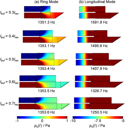
Figure 6 shows the pressure eigenmode distributions for the ring and longitudinal modes with varying l_buf, with the color scale on these plots expanded to emphasize key variations in p_n($\overrightarrow{\mathrm{r}}$) with increasing l_buf. As l_buf increases, the ring mode eigenfrequency does not change while the longitudinal eigenfrequency decreases significantly. The longitudinal mode is the n = 3 eigenmode at l_buf = 0.3l_res, but is the n = 2 eigenmode at l_buf = 0.6l_res. The sensitivity of the longitudinal mode eigenfrequency is –7.7 Hz per 1 mm increase in l_buf. This sensitivity is expected to account for the measured variability in the longitudinal eigenfrequency reported in Section 4.2.3.

Figure 6. The eigenmode pressure distributions p_n($\overrightarrow{\mathrm{r}}$) for (a) the ring mode, and (b) the longitudinal mode with varying l_buf. The color scale range has been expanded to emphasize important variations in p_n($\overrightarrow{\mathrm{r}}$) with changing l_buf. In particular, the variation in p_n($\overrightarrow{\mathrm{r}}$) within the window volumes for the ring mode and the eigenmode pressure in the two resonator pipes for the longitudinal mode is emphasized.

Figure 7 shows the predicted |p^sig(${\overrightarrow{\mathrm{r}}}_{M,\mathit{dif}})$| and |p^bck(${\overrightarrow{\mathrm{r}}}_{M,\mathit{dif}})$| over the frequency range 1320–1380 Hz for different l_buf values. For sample heating, there is little influence of l_buf on the excitation amplitude. For window heating, the |p^bck(${\overrightarrow{\mathrm{r}}}_{M,\mathit{dif}},\mathrm{ }\omega )$| show non-Lorentzian behavior caused by efficient excitation of both the longitudinal and ring modes; as discussed earlier, the overlap integral J_n for the longitudinal mode is large for the case of window heating. Importantly, the amplitude of |p^bck(${\overrightarrow{\mathrm{r}}}_{M,\mathit{dif}})$| at the ring mode eigenfrequency decreases significantly with increasing l_buf to nearly zero for l_buf = 0.7l_res. Indeed, the amplitude of |p^bck(${\overrightarrow{\mathrm{r}}}_{M,\mathit{dif}})$| for the l_buf = 0.7l_res model distribution cannot be resolved on the axis scale of Figure 7b. To explain the rapid decrease in background with increasing l_buf, the eigenmode pressure distributions in Figure 6a demonstrate that the p_n($\overrightarrow{\mathrm{r}}$) for the ring mode within the window volumes is nonzero for l_buf = 0.3l_res but decreases rapidly to zero as l_buf tends to 0.7l_res. Moreover, there is also a progressive reduction in detection of longitudinal mode excitation. To explain this latter phenomenon, the eigenmode pressure distributions in Figure 6b for the longitudinal mode show that the p_n($\overrightarrow{\mathrm{r}}$) are not equal at the location of the lower and upper microphones for l_buf = 0.3l_res and there is imperfect subtraction of detected longitudinal mode excitations upon passing the microphone signals through a differential amplifier. As l_buf increases, the p_n($\overrightarrow{\mathrm{r}}$) at the two microphone positions become equal and the differential amplifier completely removes detection of the longitudinal mode excitation.

Figure 7. The FEM-predicted frequency dependence of (a) |p^sig(${\overrightarrow{\mathrm{r}}}_{M,\mathit{dif}})$| and (b) |p^bck(${\overrightarrow{\mathrm{r}}}_{M,\mathit{dif}})$| for values of l_buf in the range 0.1 l_res – 0.7 l_res in 0.1 l_res intervals. The legend indicates the $l_{\mathit{buf}}/l_{\mathit{res}}$ ratio for different series. (c) The variation in SBR with l_buf.

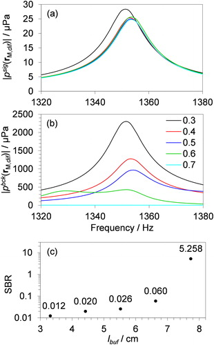
We calculated the SBR from the amplitudes of |p^sig(${\overrightarrow{\mathrm{r}}}_{M,\mathit{dif}})$| and |p^bck(${\overrightarrow{\mathrm{r}}}_{M,\mathit{dif}})$| at the ring mode eigenfrequency and Figure 7c shows the dependence of SBR on l_buf. The SBR progressively increases with l_buf to SBR > 5 at l_buf = 0.7l_res. Crucially, a 2-cm increase in l_buf from the l_buf = 0.5l_res value for our current measurement cell is expected to suppress the dominant background contribution arising from laser–window interactions. Moreover, this result demonstrates that the general rule of setting l_buf = l_res/2 is not a universal design criteria and it is important to solve rigorously the thermoviscous acoustics to determine optimal cell dimensions.

4.3.2. Optimizing the height and width of the buffer volumes

We investigated the impact of varying the buffer height (h_buf) and width (w_buf) on cell performance. The current cell has h_buf = 4.2 cm and w_buf = 2.6 cm. Given the resonator radii (r_res = 1.0 cm) and their center-to-center separation (d_res = 2.2 cm), we were restricted to lower limits of h_buf = 4.2 cm and w_buf = 2.0 cm. The simulations reported here varied h_buf from 4.5 cm to 6 cm in 0.5 cm steps, while w_buf was varied from 2.5 cm to 4 cm in 0.5 cm steps.

Figure 8 summarizes the amplitudes in the |p^sig(${\overrightarrow{\mathrm{r}}}_{\mathrm{M},\mathit{dif}},{\omega }_n)$| and |p^bck(${\overrightarrow{\mathrm{r}}}_{\mathrm{M},\mathit{dif}},{\omega }_n)$| with variation in w_buf and h_buf (frequency-dependent excitation curves are provided in Supplementary Figures S7 and S8). For sample heating, changing w_buf or h_buf had no impact on the |p^sig(${\overrightarrow{\mathrm{r}}}_{\mathrm{M},\mathit{dif}},{\omega }_n)$|. For window heating, |p^bck(${\overrightarrow{\mathrm{r}}}_{\mathrm{M},\mathit{dif}},{\omega }_n)$| decreased as w_buf increased and eigenmode simulations show that this decrease is caused by a reduction in ring eigenmode pressure within the window volumes. Meanwhile, |p^bck(${\overrightarrow{\mathrm{r}}}_{M,\mathit{dif}},{\omega }_n)$| increased for larger h_buf and eigenmode simulations show an increased ring eigenmode pressure in the window volumes for larger h_buf.

Figure 8. The variation in (a) |p^sig($\overrightarrow{\mathrm{r}}$ _M,dif, ω_n)|, (b) |p^bck($\overrightarrow{\mathrm{r}}$ _M,dif, ω_n)|, and (c) SBR with w_buf over the range 2.5–4.5 cm. Different data series are shown for the range of h_buf input to FEM simulations, from 4.5 cm to 6.0 cm in 0.5 cm steps. Lines are to guide the eye only.

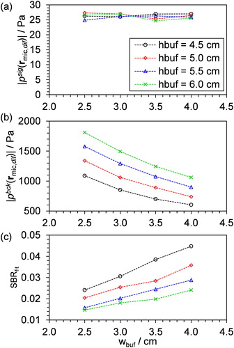
Figure 8c shows the variation in SBR with w_buf and h_buf, while Supplementary Figure S9 shows a contour plot of SBR with variation in w_buf and h_buf. Increasing w_buf is beneficial to PA cell performance, suppressing window background and increasing the SBR. For h_buf = 4.5 cm, increasing w_buf by 1 cm from 2.5 to 3.5 cm increases the SBR by 0.014 (i.e., by 60%). This is a significant increase in SBR, although not as large as the ∼130% improvement seen with increasing l_buf from 5.5 cm to 6.6 cm. Meanwhile, h_buf should be set as small as possible. There is scope to reduce h_buf by only 1 mm in our current cells if d_res and r_res are kept the same, with a 1-mm reduction in h_buf predicted to have a negligible impact on SBR.

Improving SBR by increasing w_buf or l_buf would necessarily increase the cell volume and therefore increase sample residence time. For a 1 L min⁻¹ sample flow rate, the residence time of our current cell is ∼12 s. For a 2 cm increase in l_buf (as recommended in Section 4.3.1) and a 1 cm increase in w_buf, the cell response time increases to ∼18 s. This larger cell response time is not desirable. One strategy to reduce the cell volume is to increase the fillet radii (r_fil) for the buffer volumes, although the impact of varying the fillet radius on SBR needs to be assessed. Another strategy is to reduce the radius of the upper resonator pipe. In the following sections, we investigate these strategies for reducing the cell volume and their impact on SBR.

4.3.3. Optimizing the fillet radius of the buffer volume

The current two-resonator cell has r_fil = 0.8 cm. In our model, we studied the impact on the microphone responses and SBR of varying r_fil from 0.65 cm (0.5w_buf/2) to 1.18 cm (0.9w_buf/2) in 0.13 cm (0.1w_buf/2) intervals. Supplementary Figure S10 shows cross-sections of the buffer volumes tested in this study and indicates how the total cell volume changes with r_fil, while Supplementary Figure S11 shows calculations of |p^sig($\overrightarrow{\mathrm{r}}$_mic,dif, ω)|, |p^bck($\overrightarrow{\mathrm{r}}$_mic,dif, ω)|, SBR, and response time with variation in r_fil. As r_fil increases from 0.65 cm to 1.18 cm, the total cell volume decreases by 4.3%. The ring mode excitation amplitude from sample heating is invariant with increasing r_fil, while the response from window heating shows a small decrease. The SBR increases from 0.027 to 0.032 as r_fil increases from 0.78 cm to 1.18 cm. For the same change in r_fil, there is a modest improvement in cell response time of 0.4 s. Thus, we recommend using a buffer volume with r_fil set as large as permitted by the cell geometry, with r_fil limited in our cell by the radius of the resonators and the resonator separation d_res to a maximum value of ∼r_fil = 0.9w_buf/2.

4.3.4. Optimizing the upper resonator radius and the resonator separation distance

Here, we consider the possibility of reducing the cell volume by decreasing the radius of the upper resonator (r_res,up). The radius of the lower resonator is restricted to r_res,low ≈ 1.0 cm by the need to propagate a multipass beam through the resonator, but the same constraint does not apply to the upper resonator. We used our FEM model to study the performance of the two-resonator cell for r_res,up values ranging from 0.5r_res,low to 0.9r_res,low in 0.2r_res,low intervals. Smaller values of r_res,up also allow the center-to-center resonator separation d_res to be reduced. Therefore, we varied d_res for each of the aforementioned values of r_res,up, with d_res taking values of 1.8 cm, 2.0 cm, and 2.3 cm.

Supplementary Figure S12 shows how |p^sig($\overrightarrow{\mathrm{r}}$_M,dif, ω_n)|, |p^bck($\overrightarrow{\mathrm{r}}$_M,dif, ω_n)| and SBR vary with r_res,up and d_res. We also include on these plots the values for the current cell geometry (with r_res,up = r_res,low and d_res = 2.2 cm) in addition to a point that has the same geometry as the current cell albeit with a larger upper resonator radius (r_res,up = 1.1r_res,low). Meanwhile, Supplementary Figure S13 shows the variations in the eigenmode pressure distributions for the ring and longitudinal modes for the ranges of r_res,up and d_resinput to the model. There is very little variation in the sample heating signal with changes in either r_res,up or d_res. For window heating, |p^bck($\overrightarrow{\mathrm{r}}$_M,dif, ω_n)| depends strongly on r_res,up and is minimized (SBR is maximized) for r_res,up = r_res,low, i.e., when the two resonators have the same dimensions. Indeed, the SBR is an order of magnitude higher when the resonators have equal radii compared to when r_res,up = 0.5r_res,low. The eigenmode simulations show that the decrease in |p^bck($\overrightarrow{\mathrm{r}}$_M,dif, ω_n)| as r_res,up tends to r_res,low is associated with a reduced ring mode p_n($\overrightarrow{\mathrm{r}}$) in the window volumes. Furthermore, the pressures at the two microphone locations become more similar for the longitudinal mode, leading to more effective removal of longitudinal mode detection by the differential amplifier. For the narrow 5 mm range of d_res input to the FEM model, Supplementary Figure S12 shows that there is only a small improvement in SBR by setting d_res as large as possible, with the maximum d_res limited by the buffer height. We performed simulations to investigate the impact of larger values of h_buf, on the SBR with d_res set to the maximum value (see Supplementary Figure S14). However, the results of these simulations continue to support the conclusion that h_buf should be kept as small as possible (as was concluded in Section 4.3.2) with d_res set to the maximum value.

4.3.5. Optimizing the buffer and resonator lengths for a conserved total cell length

The key conclusions from the studies above are: (1) The buffer length should be increased from the current value of 0.5l_res to 0.7l_res. This increase in l_buf improved the SBR by a factor of 200. (2) Increasing w_buf by 1 cm increased the SBR by 60%. This is a small impact on SBR compared to that achieved by increasing l_buf, while a larger w_buf will increase sample residence time. Therefore, we suggest keeping w_buf unchanged. (3) h_buf should be kept as small as possible, while d_res should be set as large as possible. (4) r_fil should be set as large as permitted by the geometry of the model, with r_fil limited by the radius of the resonators and the resonator separation d_res to a maximum value of ∼r_fil = 0.9w_buf/2. (5) The resonator radii must be equal for both resonators.

Using these design principles as a guide, we consider the dimensions of a candidate cell. We set the buffer dimensions to w_buf = 2.6 cm (unchanged), h_buf = 4.1 cm (set to minimum value), and r_fil = 1.2 cm. For the resonator dimensions, d_res = 2.1 cm and the resonator radii were reduced only slightly to 0.9 cm. The latter reduction in r_res helped reduce the total cell volume and previous studies show that smaller resonator radii improve the SBR (Bijnen, Reuss, and Harren 1996; Cotterell et al. 2019b), while a resonator radius of 0.9 cm remains large enough for our multipass laser beam to pass through the lower resonator. For the buffer length, the available space in our own instrument was restricted and making the cell longer, thus achieving criteria (1) above, was not possible. However, we note that we have not considered in our optimization studies the effect of varying the resonator lengths; l_buf could be increased at the expense of reducing the resonator length and the total cell length of 22 cm conserved through the equation: (7) $$l_{\mathit{buf}}=\frac{22.0\mathrm{ }\mathrm{cm}-\mathrm{ }{l}_{\mathit{res}}}{2}$$(7)

Thus, we performed simulations of the cell acoustic performance using the dimensions specified above and varied l_res from 8 cm to 11 cm with the total cell length constrained to 22 cm using Equation (7)(7) $$l_{\mathit{buf}}=\frac{22.0\mathrm{ }\mathrm{cm}-\mathrm{ }{l}_{\mathit{res}}}{2}$$(7) , varying the ratio l_buf/l_res over the range 0.50–0.88. Supplementary Figure S15 shows the eigenmode pressure distributions for the ring and longitudinal mode. The ring mode pressure distributions show that the eigenmode pressure within the window heating volume is close to zero for l_buf/l_res = 0.7 (l_res = 9.2 cm, l_buf = 6.4 cm). 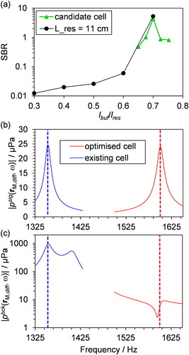Supplementary Figure S16 shows the |p^sig($\overrightarrow{\mathrm{r}}$ _mic,dif, ω)| and |p^bck($\overrightarrow{\mathrm{r}}$ _mic,dif, ω)| for sample and window heating, respectively, with simulations performed over the reduced l_buf/l_res range of 0.65–0.75 owing to the computational expense of calculating microphone responses for sample and window heating. While there are small variations in the sample heating amplitude at the ring mode frequency, the corresponding window heating amplitudes show significant variation. Importantly, Figure 9a shows that the SBR is maximized for l_buf/l_res = 0.7, consistent with the optimal l_buf/l_res ratio found in Section 4.3.1 for when the total cell length was not constrained and l_res = 11 cm. Figure 9a shows that the candidate cell with l_buf/l_res = 0.7 has an SBR of 4.35, an improvement of a factor of 170 over our current cell (l_res = 11 cm, l_buf/l_res = 0.5). Furthermore, Figures 9b and c compare the predicted frequency-dependent differential operation responses for this optimized cell with our original cell for both sample and window heating. At the ring mode eigenfrequency, the sample heating response for the optimized cell is unchanged from that of the original cell, while the window heating response is suppressed by a factor of 170 for the optimized cell. In addition to the superior SBR, the optimized cell has a reduced response time of 11.4 s for a 1 L min⁻¹ sample flow rate, 5% lower than the 12 s response time for the original cell.

Figure 9. (a) The predicted SBR with variation in l_buf/l_res for the candidate two-resonator cell for which the total cell length is constrained to 22 cm, compared with the SBR variations presented in Figure 7. (b) Comparison of the predicted frequency-dependent differential amplified microphone responses for sample heating for the original (blue curve) and optimized (red curve) PA cells. (c) Same as (b) but for window heating excitation. The ring mode eigenfrequencies for the current (dashed blue line) and optimized (dashed red line) cells are indicated.

4.4. An optimized two-resonator PA cell: model vs. measurement

We now define the final dimensions of our optimized PA cell, using the same dimensions as used in Section 4.3.6, with l_res = 9.2 cm and l_buf = 6.4 cm. The dimensions of the optimized cell are summarized in Table 2. We manufactured this cell from aluminum-alloy (Tarvin Precision Limited) and measured the cell acoustic behavior, comparing measurements with our model predictions. We recorded the microphone responses for laser heating of the cell windows, with the cell devoid of any light-absorbing sample. For these measurements, the laser amplitude modulation frequency was set to the ring mode eigenfrequency that was measured as 1604 Hz using speaker excitation of the cell. We used the same multipass optical set-up as in measurements above, using lasers with either a 405 or 658-nm optical wavelength and output powers of 260 and 100 mW, respectively. Ambient air was drawn through a Nafion dryer, NO₂, and O₃ scrubber and then the PAS cell at a flow rate of 1 L min⁻¹. We performed pressure stability tests to ensure that the cell and flow system was leak tight. The temperature of the PAS cell was maintained at 21 °C using a thermoelectric controller.

Table 2. Geometric parameters describing the optimized two-resonator PA cell.

Quantity	Value
lres	9.2 cm
rres	0.9 cm
dres	2.1 cm
lbuf	6.4 cm (0.7lres)
hbuf	4.1 cm
wbuf	2.6 cm
rfil	1.2 cm (0.9wbuf/2)
lwin	1.0 cm
rwin	1.0 cm
θB	55°

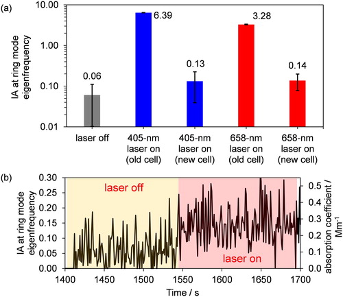
For window heating, Figure 10a shows the measured IA values for the original and optimized cells for laser wavelengths of 405 and 658 nm. For the original cell, IA_bck takes values of 6.39 and 3.28 at the 405 and 658 nm wavelengths, respectively. We note that the imaginary refractive index (directly proportional to the material absorption coefficient) for glasses tend to increase significantly as the optical wavelength approaches the UV spectrum. This increase in glass absorption is likely responsible for the larger IA_bck at 405 nm, while we also note that we observe increased scattering at the window surfaces at shorter laser wavelengths. Both the increased absorption and scattering of light at shorter wavelengths likely contribute to larger IA_bck at 405 nm compared to that at the 658 nm wavelength. The IA_bck for the optimized cell is a factor of 48 and 24 lower than that for the original cell at the 405 and 658 nm laser wavelengths, respectively. These levels of suppression in IA_bck differ from the predicted suppression in window background by a factor of 170; as we show below, IA_bck approaches a sensitivity threshold limited by ambient noise, a threshold that is not considered in our model. Crucially, the uncertainties in IA_bck for the optimized cell are within the measured IA uncertainty for measurements absent of any laser excitation (laser off), i.e., when the microphone response is dominated by ambient noise associated with sample flow, instrument vibrations, and electronic noise in the microphone measurements. Figure 10b demonstrates further the statistical insignificance of IA_bck for the optimized cell compared to ambient noise, showing a time series in IA for a 120-s period with the laser off and then for a 120-s period with the laser on. This figure also includes an indicative scale for absorption coefficient, demonstrating that the instrument sensitivity is <0.5 Mm⁻¹ and is limited by the ambient noise in microphone measurements.

Figure 10. (a) For laser heating of the Brewster windows, the measured IA at the ring mode eigenfrequency for the original (old) and optimized (new) cells for laser wavelengths of 405 and 658 nm. The mean IA for ambient noise when the laser is off is also shown. (b) A time series in the measured IA for the optimized cell when the 658-nm laser is on or off. An indicative scale is shown on the right axis for absorption coefficient based on calibration of the cell using O₃.

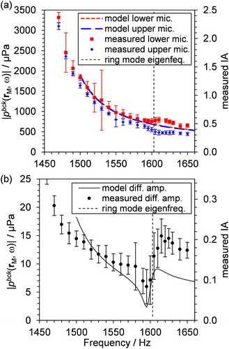
We also recorded IA_bck with variation in the laser modulation frequency for both the lower microphone, upper microphone, and for when the microphone signals were passed through a differential amplifier. The laser frequency was increased in 10 Hz intervals over the frequency range of 1450–1650 Hz, and IA_bck was recorded for 30 s at each frequency and the mean value calculated. Figure 11a compares the measured responses for the two individual microphones with the predicted response. The measured and predicted responses are in good agreement. There are small differences between the two microphone responses at the ring mode eigenfrequency (measured as 1604 Hz), with the lower microphone response increased and the upper microphone decreased compared to the model prediction. This small difference in behavior is associated with an increased excitation of the ring mode that is not included in the FEM model, with contributions from the incomplete suppression in the detection of laser–window interactions and from ambient noise. The trends in the individual microphone responses with frequency were discussed in Section 4.1.1 and are caused by the antiphase ring mode pressures at the two microphone locations; any ring mode excitation adds to the longitudinal mode contribution for the lower microphone response and subtracts from the longitudinal mode contribution for the upper microphone. Figure 11b compares the predicted and measured differential amplifier response. Again, the trends in the model predictions with changing frequency agree well with the measured response.

Figure 11. Comparison of FEM predictions of |p^bck($\overrightarrow{\mathrm{r}}$ _M, ω)| with measurements of microphone response (IA_bck) for the optimized cell for (a) lower and upper microphone responses, and (b) differential amplifier response. Error bars in (a) and (b) indicate one standard deviation in the measured IA_bck for 30 s of measurements.

Finally, Section 4.3.5 showed that our FEM model predicted the sample heating response for the optimized cell to be unchanged from that of the original cell at the ring mode eigenfrequency. Therefore, we also performed experimental measurements to confirm that the photoacoustic responses for sample heating were similar for the optimized and original cells. Previous work has comprehensively demonstrated that using ozone gas as a calibrant is an effecting approach for accurate calibration of aerosol PAS instruments (Davies et al. 2018; Cotterell et al. 2019a). Here, ozone gas is passed first through a cavity ring-down spectrometer for direct measurement of the ozone absorption coefficient prior to the ozone sample passing via serial flow to the PAS instrument for measurement of the photoacoustic response. The reader is directed to Davies et al. 2018 and Cotterell et al. 2019a for full details of our calibration procedure using this approach. Supplementary Figure S17 shows that, for the same concentration of ozone gas, the photoacoustic response of the optimized cell is 11% lower than that of the original cell. We note that the measurements using the two different cells required the multipass laser optics to be re-aligned upon installation of the new cell. This re-alignment causes small changes to the overlap integral J_n, which subsequently leads to small variations in the calibration coefficient. This change in J_n largely accounts for the 11% difference in calibration coefficient.

5. Summary

We have used finite element modeling to understand the acoustic behavior of a common two-resonator photoacoustic cell that is used by many research groups for the measurement of aerosol absorption coefficients. Our model predictions of photoacoustic pressure at the microphone locations are in excellent agreement with measurements, and understanding this acoustic response requires us to consider the excitation of both a ring and longitudinal mode. In particular, laser–window interaction sources excite the longitudinal mode very efficiently compared to the ring mode, with the longitudinal mode having a very large eigenmode pressure amplitude (thus a large overlap integral J_n) in the window volumes. However, the differential amplifier removes most of the microphone response corresponding to the excited longitudinal mode. Without differential operation, the SBR is reduced by 63%, thereby degrading the sensitivity of the PAS instrument.

We used our FEM model to optimize the geometry of the two-resonator cell, varying the dimensions of the resonators and their capping buffer volumes to maximize the SBR. In this way, we tested a very large set of cell geometries that would have taken considerable time if each cell was manufactured and tested in the laboratory. In particular, the SBR is very sensitive to the length of the buffer volumes; the SBR was increased by a factor of 150–200 from setting l_buf = 0.7l_res compared to the l_buf = 0.5l_res for our existing cell. This optimal value for l_buf challenges common misconceptions that the acoustic buffer volumes should be set at l_buf = 0.5l_res (the so-called quarter wavelength filters). Indeed, we recommend that for all but the simplest cell geometries, researchers model the acoustic behavior for their particular cell rather than relying on general design rules. Our studies show that the optimization of other cell dimensions had significantly less impact on SBR compared to varying l_buf. We measured the acoustic response of an optimized cell that was used to validate model predictions. The optimized cell suppresses the detection of laser–window interactions to a level that is within measurement uncertainty, negating the need to perform a background subtraction on aerosol photoacoustic measurements, particularly during aircraft field studies for which the window background depends strongly on pressure.

Disclosure statement

The authors declare that they have no conflict of interest.

Data availability

For data related to this paper, please contact Michael I. Cotterell ([email protected]).

Additional information

Funding

This work was supported through a Royal Society of Chemistry/Analytical Chemistry Trust Fund Tom West Fellowship awarded to Michael I. Cotterell. Jim M. Haywood and Michael I. Cotterell thank the Natural Environment Research Council for support through the CLARIFY-2017 grant [grant No. NE/L013797/1]. The Met Office funded experimental measurements. The Research Council on Norway provided further instrument support via the projects AC/BC (240372) and NetBC (244141).

References

- Ajtai, T., Á. Filep, M. Schnaiter, C. Linke, M. Vragel, Z. Bozóki, G. Szabó, and T. Leisner. 2010. A novel multi-wavelength photoacoustic spectrometer for the measurement of the UV–vis-NIR spectral absorption coefficient of atmospheric aerosols. J. Aerosol Sci. 41 (11):1020–1029. doi: 10.1016/j.jaerosci.2010.07.008.
- Arnott, W. P., J. W. Walker, H. Moosmüller, R. A. Elleman, H. H. Jonsson, G. Buzorius, W. C. Conant, R. C. Flagan, and J. H. Seinfeld. 2006. Photoacoustic insight for aerosol light absorption aloft from meteorological aircraft and comparison with particle soot absorption photometer measurements: DOE Southern Great Plains climate research facility and the coastal stratocumulus imposed perturbation experiments. J. Geophys. Res. 111 (D5):D05S02. doi: 10.1029/2005JD005964.
- Bijnen, F. G. C., J. Reuss, and F. J. M. Harren. 1996. Geometrical optimization of a longitudinal resonant photoacoustic cell for sensitive and fast trace gas detection. Rev. Sci. Instrum. 67 (8):2914–2923. doi: 10.1063/1.1147072.
- Bluvshtein, N., J. M. Flores, Q. He, E. Segre, L. Segev, N. Hong, A. Donohue, J. N. Hilfiker, and Y. Rudich. 2017. Calibration of a multi-pass photoacoustic spectrometer cell using light-absorbing aerosols. Atmos. Meas. Tech. 10(3):1203–1213. doi: 10.5194/amt-10-1203-2017.
- Bluvshtein, N., J. Michel Flores, L. Segev, and Y. Rudich. 2016. A new approach for retrieving the UV-vis optical properties of ambient aerosols. Atmos. Meas. Tech. 9 (8):3477–3490. doi: 10.5194/amt-9-3477-2016.
- Cappa, C. D., D. A. Lack, J. B. Burkholder, and A. R. Ravishankara. 2008. Bias in filter-based aerosol light absorption measurements due to organic aerosol loading: Evidence from laboratory measurements. Aerosol Sci. Technol. 42 (12):1022–1032. doi: 10.1080/02786820802389285.
- Cotterell, M. I., A. J. Orr-Ewing, K. Szpek, J. M. Haywood, and J. M. Langridge. 2019a. The impact of bath gas composition on the calibration of photoacoustic spectrometers with ozone at discrete visible wavelengths spanning the chappuis band. Atmos. Meas. Tech 12 (4):2371–2385. doi: 10.5194/amt-12-2371-2019.
- Cotterell, M. I., G. P. Ward, A. P. Hibbins, J. M. Haywood, A. Wilson, and J. M. Langridge. 2019b. Optimizing the performance of aerosol photoacoustic cells for sensitive measurements of aerosol light absorption using a finite element model. Part 1: Method validation and application to Single-Resonator multipass cells. Aerosol Sci. Technol. doi: 10.1080/02786826.2019.1650161.
- Davies, N. W., M. I. Cotterell, C. Fox, K. Szpek, J. M. Haywood, and J. M. Langridge. 2018. On the accuracy of aerosol photoacoustic spectrometer calibrations using absorption by ozone. Atmos. Meas. Tech. 11 (4):2313–2324. doi: 10.5194/amt-11-2313-2018.
- Davies, N. W., C. Fox, K. Szpek, M. I. Cotterell, J. W. Taylor, J. D. Allan, P. I. Williams, J. Trembath, J. M. Haywood, and J. M. Langridge. 2019. Evaluating biases in filter-based aerosol absorption measurements using photoacoustic spectroscopy. Atmos. Meas. Tech. 12 (6):3417–3434. doi: 10.5194/amt-12-3417-2019.
- Fischer, D., and G. D. Smith. 2018a. A portable, four-wavelength, single-cell photoacoustic spectrometer for ambient aerosol absorption. Aerosol Sci. Technol. 52 (4):393–406. doi: 10.1080/02786826.2017.1413231.
- Fischer, D., and G. D. Smith. 2018b. Can ozone be used to calibrate aerosol photoacoustic spectrometers?. Atmos. Meas. Tech. 11 (12):6419–6427. doi: 10.5194/amt-11-6419-2018.
- Foster, K., R. Pokhrel, M. Burkhart, and S. Murphy. 2019. A novel approach to calibrating a photoacoustic absorption spectrometer using polydisperse absorbing aerosol. Atmos. Meas. Tech. 12 (6):3351–3363. doi: 10.5194/amt-12-3351-2019.
- Intergovernmental Panel on Climate Change (IPCC), 2013. Climate Change 2013 The Physical Science Basis. In Contribution of Working Group I to the Fifth Assessment Report of the Intergovernmental Panel on Climate Change, ed. Stocker, T.F., D. Qin, G.-K. Plattner, M. Tignor, S.K. Allen, J. Boschung, A. Nauels, Y. Xia, V. Bex and P.M. Midgley, 1535. Cambridge: Cambridge University Press.
- Krämer, L., Z. Bozoki, and R. Niessner. 2001. Characterisation of a mobile photoacoustic sensor for atmospheric black carbon monitoring. Anal. Sci. 17:s563–s566.
- Lack, D. A., C. D. Cappa, D. S. Covert, T. Baynard, P. Massoli, B. Sierau, T. S. Bates, P. K. Quinn, E. R. Lovejoy, and A. R. Ravishankara. 2008. Bias in filter-based aerosol light absorption measurements due to organic aerosol loading: Evidence from ambient measurements. Aerosol Sci. Technol. 42 (12):1033–1041. doi: 10.1080/02786820802389277.
- Lack, D. A., C. D. Cappa, E. S. Cross, P. Massoli, A. T. Ahern, P. Davidovits, and T. B. Onasch. 2009. Absorption enhancement of coated absorbing aerosols: Validation of the photo-acoustic technique for measuring the enhancement. Aerosol Sci. Technol. 43 (10):1006–1012. doi: 10.1080/02786820903117932.
- Lack, D. A., E. R. Lovejoy, T. Baynard, A. Pettersson, and A. R. Ravishankara. 2006. Aerosol absorption measurement using photoacoustic spectroscopy: Sensitivity, calibration, and uncertainty developments. Aerosol Sci. Technol. 40 (9):697–708. doi: 10.1080/02786820600803917.
- Lack, D. A., M. S. Richardson, D. Law, J. M. Langridge, C. D. Cappa, R. J. McLaughlin, and D. M. Murphy. 2012. Aircraft instrument for comprehensive characterization of aerosol optical properties, part 2: Black and brown carbon absorption and absorption enhancement measured with photo acoustic spectroscopy. Aerosol Sci. Technol. 46 (5):555–568. doi: 10.1080/02786826.2011.645955.
- Laskin, A., J. Laskin, and S. A. Nizkorodov. 2015. Chemistry of atmospheric brown carbon. Chem. Rev. 115 (10):4335–4382. doi: 10.1021/cr5006167.
- Linke, C., I. Ibrahim, N. Schleicher, R. Hitzenberger, M. O. Andreae, T. Leisner, and M. Schnaiter. 2016. A novel single-cavity three-wavelength photoacoustic spectrometer for atmospheric aerosol research. Atmos. Meas. Tech. 9 (11):5331–5346. doi: 10.5194/amt-9-5331-2016.
- Miklós, A., P. Hess, and Z. Bozóki. 2001. Application of acoustic resonators in photoacoustic trace gas analysis and metrology. Rev. Sci. Instrum. 72 (4):1937–1955. doi: 10.1063/1.1353198.
- Moise, T., J. M. Flores, and Y. Rudich. 2015. Optical properties of secondary organic aerosols and their changes by chemical processes. Chem. Rev. 115 (10):4400–4439. doi: 10.1021/cr5005259.
- Moosmüller, H., R. K. Chakrabarty, and W. P. Arnott. 2009. Aerosol light absorption and its measurement: A review. J. Quant. Spectrosc. Radiat. Transf. 110 (11):844–878. doi: 10.1016/j.jqsrt.2009.02.035.
- Nakayama, T., Y. Kondo, N. Moteki, L. K. Sahu, T. Kinase, K. Kita, and Y. Matsumi. 2010. Size-dependent correction factors for absorption measurements using filter-based photometers: PSAP and COSMOS. J. Aerosol Sci. 41 (4):333–343. doi: 10.1016/j.jaerosci.2010.01.004.
- Nakayama, T., H. Suzuki, S. Kagamitani, Y. Ikeda, A. Uchiyama, and Y. Matsumi. 2015. Characterization of a three wavelength photoacoustic soot spectrometer (PASS-3) and a photoacoustic extinctiometer (PAX). J. Meteorol. Soc. Japan 93 (2):285–308. doi: 10.2151/jmsj.2015-016.
- Peers, F., P. Francis, C. Fox, S. J. Abel, K. Szpek, M. I. Cotterell, N. W. Davies, J. M. Langridge, K. G. Meyer, S. E. Platnick, and J. M. Haywood. 2019. Observation of absorbing aerosols above clouds over the South- East atlantic ocean from the geostationary satellite SEVIRI part 1: Method description and sensitivity. Atmos. Chem. Phys. Discuss. 19 (14):9595–9611. doi: 10.5194/acp-2018-1333.
- Radney, J. G., and C. D. Zangmeister. 2015. Measurement of gas and aerosol phase absorption spectra across the visible and near-IR using supercontinuum photoacoustic spectroscopy. Anal. Chem. 87 (14):7356–7363. doi: 10.1021/acs.analchem.5b01541.
- Rosencwaig, A. 1980. Photoacoustics and photoacoustic spectroscopy. Chichester: John Wiley and Sons, Inc.
- Sedlacek, A. J. 2006. Real-time detection of ambient aerosols using photothermal interferometry: Folded Jamin interferometer. Rev. Sci. Instrum. 77 (6):064903. doi: 10.1063/1.2205623.
- Sedlacek, A., and J. Lee. 2007. Photothermal interferometric aerosol absorption spectrometry. Aerosol Sci. Technol. 41 (12):1089–1101. doi: 10.1080/02786820701697812.
- Sharma, N., I. J. Arnold, H. Moosmüller, W. P. Arnott, and C. Mazzoleni. 2013. Photoacoustic and nephelometric spectroscopy of aerosol optical properties with a supercontinuum light source. Atmos. Meas. Tech. 6 (12):3501–3513. doi: 10.5194/amt-6-3501-2013.
- Stier, P., J. H. Seinfeld, S. Kinne, and O. Boucher. 2007. Aerosol absorption and radiative forcing. Atmos. Chem. Phys. 7 (19):5237–5261. doi: 10.5194/acp-7-5237-2007.
- Strawa, A. W., R. Castaneda, T. Owano, D. S. Baer, and B. A. Paldus. 2003. The measurement of aerosol optical properties using continuous wave cavity Ring-Down techniques. J. Atmos. Oceanic Technol. 2 0(4):454–465. doi: 10.1175/1520-0426(2003)20<454:TMOAOP > 2.0.CO;2.
- Wang, X., C. L. Heald, J. Liu, R. J. Weber, P. Campuzano-Jost, J. L. Jimenez, J. P. Schwarz, and A. E. Perring. 2018. Exploring the observational constraints on the simulation of brown carbon. Atmos. Chem. Phys. 18 (2):635–653. doi: 10.5194/acp-18-635-2018.
- Ward, G. P., A. P. Hibbins, J. R. Sambles, and J. D. Smith. 2016. Acoustic transmission through compound subwavelength slit arrays. Phys. Rev. B 94 (2):1–7. doi: 10.1103/PhysRevB.94.024304.
- Yelverton, T. L. B., M. D. Hays, B. K. Gullett, and W. P. Linak. 2014. Black carbon measurements of flame-generated soot as determined by optical, thermal-optical, direct absorption, and laser incandescence methods. Environ. Eng. Sci. 31 (4):209–215. doi: 10.1089/ees.2014.0038.
- Yu, Z., J. Assif, G. Magoon, P. Kebabian, W. Brown, W. Rundgren, J. Peck, R. Miake-Lye, D. Liscinsky, and B. True. 2017. Differential photoacoustic spectroscopic (DPAS)-based technique for PM optical absorption measurements in the presence of light absorbing gaseous species. Aerosol Sci. Technol. 51 (12):1438–1447. doi: 10.1080/02786826.2017.1363866.
- Zhang, X., H. Kim, C. L. Parworth, D. E. Young, Q. Zhang, A. R. Metcalf, and C. D. Cappa. 2016. Optical properties of wintertime aerosols from residential wood burning in Fresno, CA: Results from DISCOVER-AQ 2013. Environ. Sci. Technol. 50 (4):1681–1690. doi: 10.1021/acs.est.5b04134.
- Zuidema, P., J. Redemann, J. Haywood, R. Wood, S. Piketh, M. Hipondoka, and P. Formenti. 2016. Smoke and clouds above the southeast Atlantic: Upcoming field campaigns probe absorbing aerosol’s impact on climate. Bull. Amer. Meteor. Soc. 97 (7):1131–1135. doi: 10.1175/BAMS-D-15-00082.1.