Low Reynolds number capture of small particles on a cylinder by diffusion, interception, and inertia at subcritical Stokes numbers: Numerical calculations, correlations, and small diffusivity asymptote

Abstract

When the particle-to-target radius ratio R and the inverse Peclet number 1/P are small, particle capture by interception and diffusion by cylinders at low Reynolds numbers may be described via Friedlander’s single similarity parameter Π ≡ R·P^1/3, in the full range 0 < Π < ∞. Particle inertia may substantially enhance this capture efficiency, even at subcritical Stokes numbers S < S*∼2. We have recently shown that this inertial enhancement is the product of an ‘outer’ function E(S) accounting for inertial particle concentration enrichment along the stagnation line, and an ‘inner’ function F(Π, S) describing particle transport near the target. F(Π,S) is first computed here over its full range, (0 < Π < ∞; 0 < S < S*) by numerically solving the corresponding diffusion equation, previously analyzed only in the limits Π = 0 and Π = ∞. Two PDE solvers used (pseudo-spectral orthogonal collocation method and Mathematica’s NDSolve statement) typically agree within 0.1%, with a 0.7% maximal difference. While the previously invoked “additive capture fraction” approximation is now seen to contain errors of up to –17%, new correlations are developed here with a maximum global error of ±0.7%. We also provide a detailed numerical and asymptotic description for the universal structure of the theoretically interesting limit Π → ∞, finding an unusual algebraic decay of the small diffusive contribution to the flux in the region upstream from the critical tangency angle. We use these results to compute the substantial inertial effects reducing the penetration of toxic aerosol fumes, or improving the recovery of valuable aerosol materials (e.g., noble metals and/or semiconductors) for submicron aerosol/carrier gas cases of: Pt(s)/N₂(g) and Ge(s)/He(g).

Copyright © 2019 American Association for Aerosol Research

1. Introduction

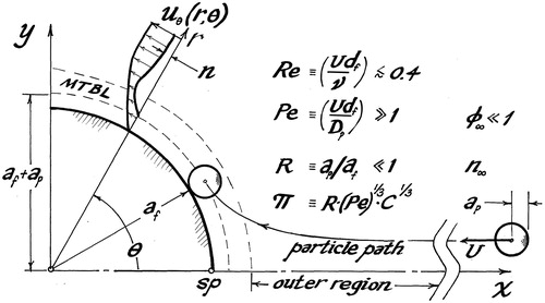
We have recently reconsidered theoretically the classical problem of particle capture by a cylinder in crossflow at modest Reynolds numbers (Re; see Nomenclature), including the simultaneous particle capture mechanisms of interception, diffusion and inertia. Under certain conditions, such as large effective Peclet number P = C(Re)·Pe (with Pe = 2a_fU/D), small interception parameter R (the ratio R = a_p/a_f between the particle and the fiber radius) and subcritical (i.e., S < S*= 2.21485) effective Stokes number S = C(Re)·Stk (with Stk = τU/a_f), the problem was reduced to solving the following convective-diffusion equation governing the local concentration n = n(s, θ) of particles in the vicinity to the cylinder surface (Fernandez de la Mora and Rosner 2019): (1) $${\Pi }^{-3}{n}_{\mathit{ss}}+s^2\left(\frac{1}{2}c\mathit{os}\theta -S\hspace{0.17em}{\text{sin}}^2\theta \right)n_s-s\mathrm{ }\hspace{0.17em}\text{sin}\hspace{0.17em}\theta n_{\theta }=2Ss\mathrm{ }\hspace{0.17em}{\text{sin}}^2\theta \mathrm{ }n.$$(1)

Equation (1)(1) $${\Pi }^{-3}{n}_{\mathit{ss}}+s^2\left(\frac{1}{2}c\mathit{os}\theta -S\hspace{0.17em}{\text{sin}}^2\theta \right)n_s-s\mathrm{ }\hspace{0.17em}\text{sin}\hspace{0.17em}\theta n_{\theta }=2Ss\mathrm{ }\hspace{0.17em}{\text{sin}}^2\theta \mathrm{ }n.$$(1) follows the original nomenclature, with P and S differing slightly from the conventional definitions of the Peclet Pe and Stokes Stk numbers by a weakly Re-dependent factor: the Oseen-Stokes function: C(Re), given by C(Re) = [1 + ln(Re^−1/2)]⁻¹. Here θ is the polar angle in a coordinate system centered with the cylinder, with θ = 0 at the forward stagnation point (see Figure 1). Π and s are the similarity variables (Equations (2)(2) $$s\equiv \left(\frac{r}{a_f}-1\right)/R$$(2) and (3)(3) $$\Pi \equiv R{P}^{1/3}$$(3) ) describing most economically the diffusion/interception problem (Friedlander 2000) (2) $$s\equiv \left(\frac{r}{a_f}-1\right)/R$$(2) (3) $$\Pi \equiv R{P}^{1/3}$$(3) s being a dimensionless radial coordinate taking a unit value one particle radius away from the cylinder wall, where the “perfect capture” boundary condition is taken to be (4) $$n\left(1,\theta \right)=0$$(4)

Figure 1. Sketch of the physical system under consideration, showing a quadrant of the cylinder (see sector with radius a_f on the left), the outer region and the mass transfer boundary layer, as well as the notation and main hypotheses considered for the relevant governing dimensionless parameters Re, Pe, and R.

The boundary condition away from the cylinder is best formulated after eliminating the right-hand side sink term in (Equation (1)(1) $${\Pi }^{-3}{n}_{\mathit{ss}}+s^2\left(\frac{1}{2}c\mathit{os}\theta -S\hspace{0.17em}{\text{sin}}^2\theta \right)n_s-s\mathrm{ }\hspace{0.17em}\text{sin}\hspace{0.17em}\theta n_{\theta }=2Ss\mathrm{ }\hspace{0.17em}{\text{sin}}^2\theta \mathrm{ }n.$$(1) ) through the new dependent variable (N) (5) $$N\equiv n{e}^{2S\left(1-\hspace{0.17em}\text{cos}\hspace{0.17em}\theta \right)}$$(5) which reduces the PDE (Equation (1)(1) $${\Pi }^{-3}{n}_{\mathit{ss}}+s^2\left(\frac{1}{2}c\mathit{os}\theta -S\hspace{0.17em}{\text{sin}}^2\theta \right)n_s-s\mathrm{ }\hspace{0.17em}\text{sin}\hspace{0.17em}\theta n_{\theta }=2Ss\mathrm{ }\hspace{0.17em}{\text{sin}}^2\theta \mathrm{ }n.$$(1) ) to: (6) $${\Pi }^{-3}{N}_{\mathit{ss}}+s^2\left(\frac{1}{2}c\mathit{os}\theta -S\hspace{0.17em}{\text{sin}}^2\theta \right)N_s-s\mathrm{ }\hspace{0.17em}\text{sin}\hspace{0.17em}\theta {\mathrm{ }N}_{\theta }=0.$$(6)

Away from the diffusion boundary layer the second order term in Equation (6)(6) $${\Pi }^{-3}{N}_{\mathit{ss}}+s^2\left(\frac{1}{2}c\mathit{os}\theta -S\hspace{0.17em}{\text{sin}}^2\theta \right)N_s-s\mathrm{ }\hspace{0.17em}\text{sin}\hspace{0.17em}\theta {\mathrm{ }N}_{\theta }=0.$$(6) may be ignored, reducing it to a first order equation solvable by the method of characteristics. In this region N is constant along the characteristics (the deterministic particle streamlines). Because both 1/P and R are small, all particles eventually captured must originate very near the stagnation point, having therefore the same value N_w prevailing near this point. Accordingly, the boundary condition away from a thin diffusion boundary layer in the vicinity of the wall is (7) $$N\to N_w=E\left(S\right) N_{\infty } \text{as} s\gg 1,$$(7) where N_∞ is the value of N (and n) far upstream, while E(S) accounts for inertial particle concentration enrichment along the stagnation line. To enable capture efficiency calculations, values of the quantity S⁻¹lnE are collected in Table 1 for several Stokes numbers.

Table 1. Compilation of E(S) calculations (Fernandez de la Mora and Rosner 2019).

S	S^–1ln E	S	S^–1ln E	S	S^–1ln E	S	S^–1ln E	S	S^–1ln E	S	S^–1ln E
2.21	5.357	2.15	3.164	1.87	2.106	1.0	1.777	0.30	1.833	0.10	1.871
2.20	4.375	2.10	2.747	1.75	1.982	0.8	1.780	0.20	1.850	0.08	1.876
2.19	3.936	2.05	2.509	1.50	1.850	0.6	1.794	0.15	1.860	0.05	1.883
2.18	3.656	2.00	2.348	1.25	1.795	0.4	1.818	0.12	1.866	0.02	1.890

As S → 0, the limit of S^–1ln E is 1.8941.

The initial condition satisfied as θ → 0 is the solution to (Equation (6)(6) $${\Pi }^{-3}{N}_{\mathit{ss}}+s^2\left(\frac{1}{2}c\mathit{os}\theta -S\hspace{0.17em}{\text{sin}}^2\theta \right)N_s-s\mathrm{ }\hspace{0.17em}\text{sin}\hspace{0.17em}\theta {\mathrm{ }N}_{\theta }=0.$$(6) ) in the stagnation region (θ = 0), which becomes an ordinary differential equation with solution (8) $$\frac{N_o\left(s,\Pi \right)}{N_w}=\frac{{\int }_1^s\hspace{0.17em}\text{exp}\hspace{0.17em}\left[-{\left(\Pi \sigma \right)}^3/6\right]d\sigma }{{\int }_1^{\mathrm{\infty }}\hspace{0.17em}\text{exp}\hspace{0.17em}\left[-{\left(\Pi \sigma \right)}^3/6\right]d\sigma }.$$(8)

Note that, although N_w itself depends on S, the starting concentration ratio (Equation (8)(8) $$\frac{N_o\left(s,\Pi \right)}{N_w}=\frac{{\int }_1^s\hspace{0.17em}\text{exp}\hspace{0.17em}\left[-{\left(\Pi \sigma \right)}^3/6\right]d\sigma }{{\int }_1^{\mathrm{\infty }}\hspace{0.17em}\text{exp}\hspace{0.17em}\left[-{\left(\Pi \sigma \right)}^3/6\right]d\sigma }.$$(8) ) is independent of the parameter S (which disappears from Equation (6)(6) $${\Pi }^{-3}{N}_{\mathit{ss}}+s^2\left(\frac{1}{2}c\mathit{os}\theta -S\hspace{0.17em}{\text{sin}}^2\theta \right)N_s-s\mathrm{ }\hspace{0.17em}\text{sin}\hspace{0.17em}\theta {\mathrm{ }N}_{\theta }=0.$$(6) when θ → 0) . For simplicity we normalize all concentrations with N_w, so the problem to be solved is to find the solution to Equation (6)(6) $${\Pi }^{-3}{N}_{\mathit{ss}}+s^2\left(\frac{1}{2}c\mathit{os}\theta -S\hspace{0.17em}{\text{sin}}^2\theta \right)N_s-s\mathrm{ }\hspace{0.17em}\text{sin}\hspace{0.17em}\theta {\mathrm{ }N}_{\theta }=0.$$(6) subject to the boundary and initial conditions: (9) $$N\left(s,\theta \right)\to 1 \text{as} s\gg 1;N\left(s=1,\theta \right)=0;N\left(s,\theta =0\right)=N_0\left(s\right).$$(9)

The principal objective of the present study is to solve numerically Equation (6)(6) $${\Pi }^{-3}{N}_{\mathit{ss}}+s^2\left(\frac{1}{2}c\mathit{os}\theta -S\hspace{0.17em}{\text{sin}}^2\theta \right)N_s-s\mathrm{ }\hspace{0.17em}\text{sin}\hspace{0.17em}\theta {\mathrm{ }N}_{\theta }=0.$$(6) subject to Equations (9)(9) $$N\left(s,\theta \right)\to 1 \text{as} s\gg 1;N\left(s=1,\theta \right)=0;N\left(s,\theta =0\right)=N_0\left(s\right).$$(9) , to provide graphical and numerical information for the local mass transfer coefficient nondimensionalized by its stagnation value (defined as T(θ, Π, S) see Equation (10)(10) $$T\left(\theta ,\Pi ,S\right)=\frac{{\left[n_s\left(\theta ,\Pi ,S\right)\right]}_{s=1}}{{\left[n_s\left(0,\Pi \right)\right]}_{s=1}}=\frac{e^{-2S\left(1-\hspace{0.17em}\text{cos}\hspace{0.17em}\theta \right)}{\left[N_s\left(\theta ,\Pi ,S\right)\right]}_{s=1}}{Z\left(\Pi \right)};$$(10) ), and the total dimensionless mass transfer coefficient F(Π, S) (see Equation (11)(11) $$F\left(\Pi ,S\right)=\frac{1}{2\pi }{\int }_{\theta }^{2\pi }T\left(\theta ,\Pi ,S\right)d\theta .$$(11) ). These two transport coefficients are related to the solution to Equation (6)(6) $${\Pi }^{-3}{N}_{\mathit{ss}}+s^2\left(\frac{1}{2}c\mathit{os}\theta -S\hspace{0.17em}{\text{sin}}^2\theta \right)N_s-s\mathrm{ }\hspace{0.17em}\text{sin}\hspace{0.17em}\theta {\mathrm{ }N}_{\theta }=0.$$(6) as follows: (10) $$T\left(\theta ,\Pi ,S\right)=\frac{{\left[n_s\left(\theta ,\Pi ,S\right)\right]}_{s=1}}{{\left[n_s\left(0,\Pi \right)\right]}_{s=1}}=\frac{e^{-2S\left(1-\hspace{0.17em}\text{cos}\hspace{0.17em}\theta \right)}{\left[N_s\left(\theta ,\Pi ,S\right)\right]}_{s=1}}{Z\left(\Pi \right)};$$(10) (11) $$F\left(\Pi ,S\right)=\frac{1}{2\pi }{\int }_{\theta }^{2\pi }T\left(\theta ,\Pi ,S\right)d\theta .$$(11) where the normalizing denominator in Equation (10)(10) $$T\left(\theta ,\Pi ,S\right)=\frac{{\left[n_s\left(\theta ,\Pi ,S\right)\right]}_{s=1}}{{\left[n_s\left(0,\Pi \right)\right]}_{s=1}}=\frac{e^{-2S\left(1-\hspace{0.17em}\text{cos}\hspace{0.17em}\theta \right)}{\left[N_s\left(\theta ,\Pi ,S\right)\right]}_{s=1}}{Z\left(\Pi \right)};$$(10) does not depend on S and is (12) $$Z\left(\Pi \right)={\left[n_s\left(0,\Pi \right)\right]}_{s=1}=\frac{\hspace{0.17em}\text{exp}\hspace{0.17em}\left[-{\Pi }^3/6\right]}{{\int }_1^{\infty }\hspace{0.17em}\text{exp}\hspace{0.17em}\left[-{\left(\Pi s\right)}^3/6\right]ds}=\frac{3^{2/3}\Pi \hspace{0.17em}\text{exp}\hspace{0.17em}\left[-{\Pi }^3/6\right]}{2^{1/3}\Gamma \left(1/3,{\Pi }^3/6\right)},$$(12) and Γ is the incomplete gamma function.

2. Numerical analysis

Two numerical approaches were used: the Wolfram Mathematica PDE-solver NDSolve and the pseudo-spectral orthogonal collocation method.

2.1. Mathematica PDE-solver

Calculations were initially based on the computer program Wolfram Mathematica, with the following integration statement (see sample program in the online supplementary information): (13) $$\begin{array}{c}\text{NDSolve}\left[\right\{{\Pi }^{-3}D\left[N\right[\theta ,s\left],s,s\right]+s^2(\hspace{0.17em}\text{Cos}[\theta \left]/2–S \hspace{0.17em}\text{Sin}\hspace{0.17em}\right[\theta \left]{}^2)D\right[N[\theta ,s\left],s\right]\\ ==s \hspace{0.17em}\text{Sin}\left[\theta \left] D\right[N\right[\theta ,s],\theta \left], N\right[\theta ,1\left]==0, N\right[\theta ,\Delta \left]==1, N\right[{\theta }_o, s\left]==N_o\right[s\left]\}, N\right[\theta , s], \{\theta ,{\theta }_o,{\theta }_1\}, \{s, 1,\Delta \}]\end{array}$$(13)

As indicated in the Mathematica statement Equation (13)(13) $$\begin{array}{c}\text{NDSolve}\left[\right\{{\Pi }^{-3}D\left[N\right[\theta ,s\left],s,s\right]+s^2(\hspace{0.17em}\text{Cos}[\theta \left]/2–S \hspace{0.17em}\text{Sin}\hspace{0.17em}\right[\theta \left]{}^2)D\right[N[\theta ,s\left],s\right]\\ ==s \hspace{0.17em}\text{Sin}\left[\theta \left] D\right[N\right[\theta ,s],\theta \left], N\right[\theta ,1\left]==0, N\right[\theta ,\Delta \left]==1, N\right[{\theta }_o, s\left]==N_o\right[s\left]\}, N\right[\theta , s], \{\theta ,{\theta }_o,{\theta }_1\}, \{s, 1,\Delta \}]\end{array}$$(13) , the integration domain used was the rectangle θ_o < θ < θ₁; 1 < s < Δ, where θ_o typically took the value 10⁻⁵. The quantity θ₁ was often taken to be smaller than the natural upper limit π, especially when inertial centrifugation brought the particle flux at the wall to exponentially small values well below θ = π (Figure 2). A sound selection of the boundary layer thickness variable Δ was found to be vital, especially for Π > 1.2, when the diffusive region is thin and the calculation fails when the assigned Δ is excessive (e.g., when Π = 16, Δ had to exceed unity by as little as 0.015). Convergence at Π > 16 was complicated because Mathematica’s limited numerical accuracy in the calculation of the initial condition N[θ_o, s] = N_o[s] for large Π values hampered the high accuracy goal usually expected by Mathematica’s numerical differential equation solver NDSolve. An alternative description of N_o could be easily handled by using asymptotic expressions for the incomplete gamma function in the definition of N_o[s] (see Equations (8)(8) $$\frac{N_o\left(s,\Pi \right)}{N_w}=\frac{{\int }_1^s\hspace{0.17em}\text{exp}\hspace{0.17em}\left[-{\left(\Pi \sigma \right)}^3/6\right]d\sigma }{{\int }_1^{\mathrm{\infty }}\hspace{0.17em}\text{exp}\hspace{0.17em}\left[-{\left(\Pi \sigma \right)}^3/6\right]d\sigma }.$$(8) and (12)(12) $$Z\left(\Pi \right)={\left[n_s\left(0,\Pi \right)\right]}_{s=1}=\frac{\hspace{0.17em}\text{exp}\hspace{0.17em}\left[-{\Pi }^3/6\right]}{{\int }_1^{\infty }\hspace{0.17em}\text{exp}\hspace{0.17em}\left[-{\left(\Pi s\right)}^3/6\right]ds}=\frac{3^{2/3}\Pi \hspace{0.17em}\text{exp}\hspace{0.17em}\left[-{\Pi }^3/6\right]}{2^{1/3}\Gamma \left(1/3,{\Pi }^3/6\right)},$$(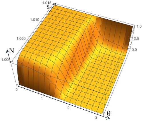12) ). However, this was not pursued because the case with Π = 16 is already close enough to the analytically tractable limit Π = ∞ to: (i) confirm the accuracy of the numerical calculation at Π = 16, and (ii) provide an excellent numerical description of the asymptotic region at large Π. While the selection of a small or moderate Δ facilitates the calculation at small enough θ, naturally the boundary layer widens with θ, requiring a domain large enough for the boundary condition N(s = ∞) = 1 to be reached. Under all conditions, deterministic particle trajectories become tangent to the cylinder at a certain critical angle θ*(S), beyond which particles have to diffuse against convection across the increasingly wider region separating this critical trajectory from the cylinder. The peculiarity of this situation at large Π is illustrated in Figure 2, for S = 0 (θ* = π/2), where the small diffusivity (Π = 16) results in a precipitous decay of N to the right of the critical trajectory. One can see that there is a finite deposition rate slightly to the right of θ = π/2. To avert inaccuracies in the calculation due to an unsatisfied outer boundary condition N → 1, we have increased Δ sufficiently for the boundary condition to be met at all values of θ associated with a finite deposition (Figure 2). This required a certain level of numerical experimentation until a Δ value providing a seemingly sensible N profile was identified. A more quantitative assurance of the reliability of a calculation can be obtained from the independence of the global deposition rate F(Π, S) on the width chosen for the integration domain.

Figure 2. Example of a concentration profile N(θ, s) for the case S = 0, Π = 16, when the region θ < π/2 (where convection moves particles towards the wall) exhibits a very thin diffusive boundary layer, while the region θ > π/2 (where convection moves particles away from the wall) exhibits a sharply defined dust-free-region to the right of the critical trajectory tangent to the cylinder.

Further confirmation of the reliability of the numerical calculation may be drawn from Figure 3b, comparing the analytical solution for Π = ∞ [T(θ, ∞, 0) = cosθ) with the numerical calculation for T(θ, 16, 0). In this case the diffusive region is particularly thin at small θ, where the largest inaccuracies should be expected. Nonetheless, the numerical solution approaches closely cosθ in this region. As anticipated, the diffusive transport contributions are restricted to a small domain in the vicinity of the critical angle. To the right of this angle a convective drift velocity associated with centrifugal forces quickly suppresses the ability of diffusion to add to the particle flux. To the left of this critical angle the deposition is quickly dominated by convection and interception (dashed curve). Figure 3a shows the widening of the diffusive region as Π ceases to be large, the diffusive region widens well beyond the close vicinity to the corner (Figure 3a). Notice that the gray curve decays exponentially into its right Π→∞ asymptote, but far more slowly (apparently algebraically) into its left asymptote. This peculiarity will be analyzed in detail in Section 5.

Figure 3. Local deposition rate function T(θ, Π, 0) in the absence of inertial effects. (b) Comparison of the (dashed) analytical solution, T(θ, ∞, 0) = cosθ with the (gray) numerical solution for Π = 16, showing excellent agreement except for the smoothing of the singular corner region near θ = π/2. (a) Π-dependence of T(θ, Π, 0) for (top to bottom) Π = 1, 1.5, 2, 3, 4, 6, 8, 10, and 16.

No convergence issues were encountered in the limit Π ≪ 1, as long as large enough Δ values were assigned for the outer boundary condition to be met. For instance, at the lowest value studied, Π = 0.001, Δ had to be as large as 1000. The accuracy of the Mathematica calculation in this limit is tested over all the relevant S range in Figure 4, by comparing the numerical T(θ, 0.01, S) with the analytically known T(θ, 0, S).

Figure 4. Normalized local particle deposition rate versus polar angle θ at various Stokes numbers. Comparison between the numerical solution for Π = 0.01 (gray continuous lines) and the analytical solution for Π = 0 (black dashed lines). From top to bottom, S = 0, 0.1, 0.2, 0.3, 0.4, 0.6, 0.8, 1, 1.2, 1.4, 1.6, 1.8, and 2.

2.2. Pseudo-spectral orthogonal collocation method

Equation (6)(6) $${\Pi }^{-3}{N}_{\mathit{ss}}+s^2\left(\frac{1}{2}c\mathit{os}\theta -S\hspace{0.17em}{\text{sin}}^2\theta \right)N_s-s\mathrm{ }\hspace{0.17em}\text{sin}\hspace{0.17em}\theta {\mathrm{ }N}_{\theta }=0.$$(6) has been also solved using the pseudo-spectral orthogonal collocation method (see, e.g., Boyd 2000; Gottlieb and Orszag 1977; Quarteroni and Valli 2008) in terms of a mapped angular variable defined by x = cosθ (with values in [–1, 1]), and a mapped radial variable z defined by the relation z = 1 – [1 + Π (s – 1)]⁻¹. This way, the semi-infinite radial interval in terms of s is mapped to the finite [0, 1] interval in terms of z (i.e., z(s = 1) = 0, z(s = ∞) = 1), thus avoiding the use of extra parameters as an artificial finite maximal radius Δ. Moreover, since dz/ds is proportional to Π, the mapped variable z takes into account the large boundary layer thickness found for small values of Π, thus allowing for accurate results for all values of Friedlander’s single similarity parameter Π.

According to the orthogonal collocation method the function N(θ, s) is approximated, in terms of the mapped variables (x, z) by means of a truncated expansion of orthogonal polynomials given by (14) $$N\left(x,z\right)={\sum }_{i=1}^{k_x}{\sum }_{j=1}^{k_z}{N}_{\mathit{ij}}{\varphi }_i\left(x\right){\varphi }_j\left(z\right)with{N}_{\mathit{ij}}=N\left(x_i,z_j\right)$$(14) where x_i (i = 1, 2, …, k_x) and z_j (j = 1, 2, …, k_z) are the collocation abscissae used for each variable. In the case of variable x the collocation abscissae used are given by the corresponding nodes of the Chebyshev-Radau quadrature formula, which includes the boundary value x = 1, corresponding to θ = 0. On the other hand, the collocation abscissae used for variable z are given by the Chebyshev-Lobatto quadrature formula, thus including both boundaries z = 0 and z = 1 as collocation abscissae. Hence, the former truncated expansion (Equation (14)(14) $$N\left(x,z\right)={\sum }_{i=1}^{k_x}{\sum }_{j=1}^{k_z}{N}_{\mathit{ij}}{\varphi }_i\left(x\right){\varphi }_j\left(z\right)with{N}_{\mathit{ij}}=N\left(x_i,z_j\right)$$(14) ) allows for the application of all boundary conditions given by Equation (9)(9) $$N\left(s,\theta \right)\to 1 \text{as} s\gg 1;N\left(s=1,\theta \right)=0;N\left(s,\theta =0\right)=N_0\left(s\right).$$(9) . On the other hand, the functions ϕ_i(x) and ϕ_j(z) are the (respectively) ith and jth cardinal basis function (i.e., ϕ_i(x_m) = δ_im) related to the Chebyshev-Radau (respectively, Chebyshev-Lobatto) quadrature formula (see Boyd 2000; Hildebrand 2013). Inserting Equation (14)(14) $$N\left(x,z\right)={\sum }_{i=1}^{k_x}{\sum }_{j=1}^{k_z}{N}_{\mathit{ij}}{\varphi }_i\left(x\right){\varphi }_j\left(z\right)with{N}_{\mathit{ij}}=N\left(x_i,z_j\right)$$(14) in Equation (6)(6) $${\Pi }^{-3}{N}_{\mathit{ss}}+s^2\left(\frac{1}{2}c\mathit{os}\theta -S\hspace{0.17em}{\text{sin}}^2\theta \right)N_s-s\mathrm{ }\hspace{0.17em}\text{sin}\hspace{0.17em}\theta {\mathrm{ }N}_{\theta }=0.$$(6) written in terms of the mapped variables (x, z) and evaluating at the collocation abscissae, allows re-writing Equation (6)(6) $${\Pi }^{-3}{N}_{\mathit{ss}}+s^2\left(\frac{1}{2}c\mathit{os}\theta -S\hspace{0.17em}{\text{sin}}^2\theta \right)N_s-s\mathrm{ }\hspace{0.17em}\text{sin}\hspace{0.17em}\theta {\mathrm{ }N}_{\theta }=0.$$(6) as an easily solved linear algebraic problem, yielding the values of N(x, z) at the corresponding collocation abscissae (i.e., the coefficients N_ij in the truncated pseudo-spectral expansion Equation (14)(14) $$N\left(x,z\right)={\sum }_{i=1}^{k_x}{\sum }_{j=1}^{k_z}{N}_{\mathit{ij}}{\varphi }_i\left(x\right){\varphi }_j\left(z\right)with{N}_{\mathit{ij}}=N\left(x_i,z_j\right)$$(14) ).

In the most demanding cases (found for large Π-values) a relatively large number of abscissae was needed (k_x = 56 (interior abscissae) + 1 (boundary abscissa) for x = cosθ, and k_z = 65 (interior abscissae) + 2 (boundary abscissae) for the mapped radial variable z. Hence, this number of abscissae has been used in all the cases. As a consequence the number of coefficients N_ij considered in the truncated pseudo-spectral expansion Equation (14)(14) $$N\left(x,z\right)={\sum }_{i=1}^{k_x}{\sum }_{j=1}^{k_z}{N}_{\mathit{ij}}{\varphi }_i\left(x\right){\varphi }_j\left(z\right)with{N}_{\mathit{ij}}=N\left(x_i,z_j\right)$$(14) is given by (56 + 1)×(65 + 2) = 3819, and the solution of Equation (6)(6) $${\Pi }^{-3}{N}_{\mathit{ss}}+s^2\left(\frac{1}{2}c\mathit{os}\theta -S\hspace{0.17em}{\text{sin}}^2\theta \right)N_s-s\mathrm{ }\hspace{0.17em}\text{sin}\hspace{0.17em}\theta {\mathrm{ }N}_{\theta }=0.$$(6) was provided by the inversion of a 3819 × 3819 matrix.

In all the cases considered, which included values of S between 0 and 2.1 and Π between 0 and 20, the results for F found by means of the former implementation of the orthogonal collocation method differed typically by ±0.1% from those following the algorithm implemented by the NDSolve Mathematica function. Differences as large as ±0.36%, were found in a few exceptional cases corresponding to S = 0. These differences are imperceptible for most purposes of the present study. An exception, however, arises in Section 5, where the considerably greater accuracy achieved by the pseudospectral orthogonal collocation method is essential to provide an accurate description of the small diffusive contributions when interception dominates.

3. Numerical results and discussion

3.1. The inertialess limit

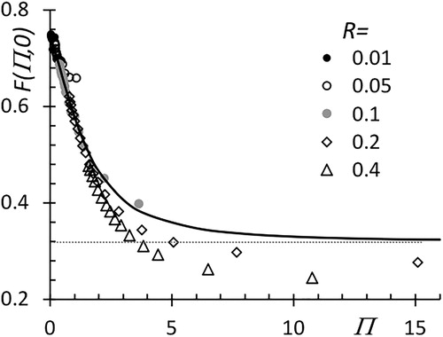
Figure 5 shows our numerical results as a continuous black line for F(Π, 0) in the limit S = 0. The data symbols also included in the figure are from prior computations by Yeh and Liu (1974) in the limit S = 0. These results, originally reported in terms of the variables R and P, have been converted to the self-similar variables F and Π by Fernandez de la Mora and Rosner (2019). The earlier numerical data collapse reasonably well into a single curve at moderate values of Π, though not so well above Π > 2. One main reason for the loss of self-similarity at larger Π is the corresponding relatively large values of R, which invalidate the near-wall description of the fluid velocity field necessary for the self-similarity law to apply. Our numerical results for S = 0 agree well with Yeh and Liu (1974), but only at Π below 1.5–2, where the various symbols also agree among themselves. As previously demonstrated by Figure 3b, the large Π asymptote of our numerical calculations approach accurately the expected analytical behavior as Π → ∞.

Figure 5. Function F(Π, 0) for deposition of particles without inertia. The continuous line is the present numerical solution. The data points are numerical calculations of Yeh and Liu (1974), converted into self-similar form by Fernandez de la Mora and Rosner (2019).

The main outcome of these numerical calculations is Table 2, collecting computed F(Π, S) data, also graphed in Figures 6 and 7 (with S and Π, respectively, in the abscissa). One can see in Figure 6 that the numerical data fill smoothly the formerly uncharacterized space between the Π = 0 and Π = ∞ asymptotes, given by Equation (11)(11) $$F\left(\Pi ,S\right)=\frac{1}{2\pi }{\int }_{\theta }^{2\pi }T\left(\theta ,\Pi ,S\right)d\theta .$$(11) (Fernandez de la Mora and Rosner 2019). (15) $$T\left(\theta ,\Pi =0,S\right)=\frac{\sqrt{s\mathit{in}\theta }{e}^{-3S\left(1-\hspace{0.17em}\text{cos}\hspace{0.17em}\theta \right)}}{{\left(\frac{3}{2}{\int }_0^{\theta }\sqrt{s\mathit{in}\theta \mathrm{\text{'}}}{e}^{-3S\left(1-\hspace{0.17em}\text{cos}\hspace{0.17em}\theta \mathrm{\text{'}}\right)}d\theta \mathrm{\text{'}}\right)}^{1/3}}$$(15) (16) $$T\left(\theta ,\Pi =\mathrm{\infty },S\right)=\left(\hspace{0.17em}\text{cos}\hspace{0.17em}\theta -2S\hspace{0.17em}{\text{sin}}^2\theta \right)e^{-2S\left(1-\hspace{0.17em}\text{cos}\hspace{0.17em}\theta \right)}.$$(16)

Figure 6. Calculated global deposition rate function F(Π,S) with S as the abscissa. The upper and lower boundaries are the asymptotes F(0, S) and F(∞, S), respectively.

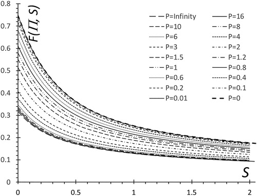
Figure 7. Calculated global deposition function F(Π,S) with Π as the abscissa, and S = (top to bottom) 0, 0.1, 0.2, 0.3, 0.4, 0.5, 0.6, 0.8, 1.0, 1.2, 1.4, 1.6, 1.8, and 2.0. Asymptotic behaviors in the small and large Π limits (Equations (17)(17) $$F\left(\Pi ,S\right)\simeq F\left(\mathrm{\infty },S\right)+A\left(S\right){\Pi }^{-2}; \text{for} \Pi \gg 1,$$(17) and (18)(18) $$F\left(\Pi ,S\right)\simeq F\left(0,S\right)-B\left(S\right)\Pi ; \text{for} \Pi \ll 1,$$(18) ) are also shown as gray lines, matching the corresponding numerical results found in each limit.

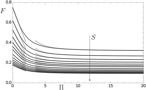
Table 2. Computed dependence of F(Π,S) on its two variables, based on the orthogonal collocation method.

Π	S = 0	S = 0.1	S = 0.2	S = 0.3	S = 0.4	S = 0.5	S = 0.6	S = 0.8	S = 1.0	S = 1.2	S = 1.4	S = 1.6	S = 1.8	S = 2
∞	0.31831	0.26577	0.22991	0.20443	0.18548	0.17079	0.15904	0.14125	0.12829	0.11832	0.11035	0.10380	0.09829	0.09357
16	0.32436	0.26959	0.23312	0.20721	0.18793	0.17301	0.16107	0.14301	0.12988	0.11977	0.11169	0.10501	0.09956	0.09461
15	0.32502	0.27009	0.23354	0.20757	0.18825	0.17330	0.16133	0.14324	0.13008	0.11995	0.11185	0.10518	0.09966	0.09478
14	0.32574	0.27073	0.23407	0.20801	0.18865	0.17366	0.16166	0.14352	0.13033	0.12018	0.11206	0.10539	0.09983	0.09497
12	0.32780	0.27241	0.23547	0.20923	0.18973	0.17464	0.16255	0.14431	0.13101	0.12079	0.11264	0.10596	0.10032	0.09548
10	0.33109	0.27514	0.23778	0.21120	0.19148	0.17620	0.16399	0.14554	0.13212	0.12182	0.11358	0.10682	0.10113	0.09628
8	0.33692	0.27998	0.24181	0.21468	0.19452	0.17896	0.16650	0.14772	0.13407	0.12358	0.11520	0.10833	0.10256	0.09761
6	0.34862	0.28977	0.24988	0.22160	0.20061	0.18441	0.17149	0.15202	0.13789	0.12705	0.11846	0.11134	0.10537	0.10029
4	0.37698	0.31343	0.26946	0.23825	0.21518	0.19744	0.18334	0.16218	0.14693	0.13526	0.12598	0.11839	0.11201	0.10654
3	0.40805	0.33920	0.29093	0.25642	0.23094	0.21144	0.19601	0.17301	0.15649	0.14388	0.13394	0.12579	0.11893	0.11305
2	0.46706	0.38796	0.33163	0.29086	0.26065	0.23761	0.21952	0.19282	0.17389	0.15959	0.14832	0.13912	0.13146	0.12495
1.5	0.51526	0.42772	0.36485	0.31901	0.28489	0.25886	0.23847	0.20861	0.18762	0.17190	0.15956	0.14954	0.14118	0.13404
1.2	0.55253	0.45847	0.39056	0.34081	0.30366	0.27529	0.25310	0.22072	0.19811	0.18126	0.16807	0.15738	0.14856	0.14101
1.1	0.56647	0.46997	0.40018	0.34897	0.31070	0.28145	0.25858	0.22523	0.20201	0.18472	0.17122	0.16032	0.15128	0.14357
1.0	0.58117	0.48210	0.41033	0.35759	0.31812	0.28795	0.26435	0.22999	0.20610	0.18836	0.17454	0.16337	0.15412	0.14627
0.8	0.61270	0.50812	0.43210	0.37608	0.33407	0.30191	0.27676	0.24020	0.21488	0.19615	0.18162	0.16990	0.16019	0.15195
0.6	0.64660	0.53609	0.45553	0.39598	0.35124	0.31695	0.29012	0.25118	0.22430	0.20450	0.18916	0.17684	0.16666	0.15804
0.4	0.68182	0.56515	0.47986	0.41667	0.36909	0.33258	0.30401	0.26256	0.23405	0.21311	0.19695	0.18400	0.17332	0.16428
0.2	0.71658	0.59384	0.50389	0.43709	0.38670	0.34800	0.31769	0.27376	0.24360	0.22153	0.20454	0.19097	0.17980	0.17035
0.1	0.73301	0.60739	0.51523	0.44673	0.39500	0.35525	0.32412	0.27900	0.24806	0.22546	0.20807	0.19420	0.18280	0.17316
0.01	0.74813	0.61986	0.52566	0.45558	0.40262	0.36190	0.33000	0.28378	0.25212	0.22901	0.21126	0.19712	0.18550	0.17570
0	0.74691	0.61887	0.52490	0.45500	0.40219	0.36159	0.32977	0.28367	0.25206	0.22899	0.21127	0.19713	0.18550	0.17573
A(S)	1.24550	0.93723	0.78550	0.67683	0.59833	0.53979	0.49391	0.42860	0.38046	0.34573	0.31993	0.30676	0.27731	0.27769
B(S)	0.1689	0.1394	0.1167	0.0992	0.0855	0.0748	0.0664	0.0544	0.0465	0.0410	0.0370	0.0340	0.0316	0.0296

The rows for Π = 0 and Π=∞ are from analytic expressions (Equations (11)(11) $$F\left(\Pi ,S\right)=\frac{1}{2\pi }{\int }_{\theta }^{2\pi }T\left(\theta ,\Pi ,S\right)d\theta .$$(11) , (15)(15) $$T\left(\theta ,\Pi =0,S\right)=\frac{\sqrt{s\mathit{in}\theta }{e}^{-3S\left(1-\hspace{0.17em}\text{cos}\hspace{0.17em}\theta \right)}}{{\left(\frac{3}{2}{\int }_0^{\theta }\sqrt{s\mathit{in}\theta \mathrm{\text{'}}}{e}^{-3S\left(1-\hspace{0.17em}\text{cos}\hspace{0.17em}\theta \mathrm{\text{'}}\right)}d\theta \mathrm{\text{'}}\right)}^{1/3}}$$(15) , and (16(16) $$T\left(\theta ,\Pi =\mathrm{\infty },S\right)=\left(\hspace{0.17em}\text{cos}\hspace{0.17em}\theta -2S\hspace{0.17em}{\text{sin}}^2\theta \right)e^{-2S\left(1-\hspace{0.17em}\text{cos}\hspace{0.17em}\theta \right)}.$$(16) )). The two bottom rows, based on linear fits to the table data, describe F(Π,S) as Π→0 and Π→∞, as described by Equations (17)(17) $$F\left(\Pi ,S\right)\simeq F\left(\mathrm{\infty },S\right)+A\left(S\right){\Pi }^{-2}; \text{for} \Pi \gg 1,$$(17) and (18)(18) $$F\left(\Pi ,S\right)\simeq F\left(0,S\right)-B\left(S\right)\Pi ; \text{for} \Pi \ll 1,$$(18) .

The first and last three rows of Table 2 summarize the behavior in the vicinity of both asymptotes, given by: (17) $$F\left(\Pi ,S\right)\simeq F\left(\mathrm{\infty },S\right)+A\left(S\right){\Pi }^{-2}; \text{for} \Pi \gg 1,$$(17) (18) $$F\left(\Pi ,S\right)\simeq F\left(0,S\right)-B\left(S\right)\Pi ; \text{for} \Pi \ll 1,$$(18) where the asymptote (17) corresponding to large Π-values becomes accurate for Π > 6, and the asymptote (18) corresponding to small Π-values remains accurate for all values of Π in the interval 0 ≤ Π ≤ 1.2 (see Figure 7). The coefficients A(S) and B(S) in Equations (17)(17) $$F\left(\Pi ,S\right)\simeq F\left(\mathrm{\infty },S\right)+A\left(S\right){\Pi }^{-2}; \text{for} \Pi \gg 1,$$(17) and (18)(18) $$F\left(\Pi ,S\right)\simeq F\left(0,S\right)-B\left(S\right)\Pi ; \text{for} \Pi \ll 1,$$(18) are approximately A(S) = [∂F(Π,S)/∂Π⁻²]_Π=∞, B(S) = [∂F(Π,S)/∂Π]_Π=0, though the values reported in the table are obtained from linear fits to the tabulated data (including the exact values at Π = 0 and ∞). The A(S) coefficient fixing the behavior as Π → ∞ is obtained from a linear fit (vs. Π²) for Π > 10. The slope B(S) at the origin is a linear fit to all the data in the interval 0 ≤ Π ≤ 1, taking advantage of the wide extent of the initial linear region. The aforementioned region of validity of the asymptotic descriptions Equations (17)(17) $$F\left(\Pi ,S\right)\simeq F\left(\mathrm{\infty },S\right)+A\left(S\right){\Pi }^{-2}; \text{for} \Pi \gg 1,$$(17) and (18)(18) $$F\left(\Pi ,S\right)\simeq F\left(0,S\right)-B\left(S\right)\Pi ; \text{for} \Pi \ll 1,$$(18) may be seen in Figure 7 to be approximately as indicated (i.e., Π > 6 and Π ≤ 1.2, respectively), with gray lines corresponding in Figure 7 to the asymptotic descriptions. Note that the value of B(S) depends on the Π range of F values used for the linear fitting. The representation of Figure 7 is essentially equivalent to that of Figure 6, but the availability of analytic expressions for F(0, S) and F(∞, S), together with the tabulated A(S) and B(S) functions, makes them more suitable for developing accurate correlations which are easier to use than, say, a two-dimensional interpolation based on Table 2.

4. Comparisons with earlier approximations and correlations for fibrous filter performance calculations

The availability of numerical values for the function F(Π,S) opens the door to testing the accuracy of previously proposed approximations, including the widely-used “additive capture fraction” approximation (i.e., η_a ≈ η_cap(‘pure’ convective-diffusion) + η_cap(‘pure’ interception)) exploited by Lee and Liu (1982) in the limit S = 0, generalized below for finite S as: (19) $$Z\left(\Pi \right)F_a\left(\Pi ,S\right)\simeq Z_0\left(\Pi \right)F\left(0,S\right)+Z_{\mathrm{\infty }}\left(\Pi \right)F\left(\mathrm{\infty },S\right),$$(19) where Z₀(Π) and Z_∞(Π) are the limits of Z(Π) as its argument tends to either 0 or ∞, defined as: (20a, b) $$Z_0\left(\Pi \right)\equiv \frac{3\Pi }{\sqrt[3]{6}\Gamma \left(1/3\right)}; Z_{\infty }\left(\Pi \right)\equiv \frac{1}{2}{\Pi }^3.$$(20a, b)

These equations were used to predict the augmentation factor in single-fiber capture fraction to be expected in the presence of subcritical particle inertia—i.e., the “S-effect” factor given by: E(S)·F(Π,S)/F(Π, 0). In order to facilitate such calculations E(S) data are included in Table 2.

Using the orthogonal collocation results of Table 2 we find that Equation (19)(19) $$Z\left(\Pi \right)F_a\left(\Pi ,S\right)\simeq Z_0\left(\Pi \right)F\left(0,S\right)+Z_{\mathrm{\infty }}\left(\Pi \right)F\left(\mathrm{\infty },S\right),$$(19) underpredicts F(Π,S) in the whole S, Π domain. The errors exceed –10% and when 0.5 < Π < 2.5, and reach a maximum of –17% at Π ≃ 1. There is, however, very little S-dependence of this error, making Equation (19)(19) $$Z\left(\Pi \right)F_a\left(\Pi ,S\right)\simeq Z_0\left(\Pi \right)F\left(0,S\right)+Z_{\mathrm{\infty }}\left(\Pi \right)F\left(\mathrm{\infty },S\right),$$(19) a precise predictor of the “S-effect”-ratio.

For practical filtration performance prediction purposes it would be valuable to report a convenient correlation equation which successfully represents the complete bivariate function F(Π,S) provided in Table 2. Because exact results for the limiting functions F(0, S) and F(∞, S) are available (Equations (15)(15) $$T\left(\theta ,\Pi =0,S\right)=\frac{\sqrt{s\mathit{in}\theta }{e}^{-3S\left(1-\hspace{0.17em}\text{cos}\hspace{0.17em}\theta \right)}}{{\left(\frac{3}{2}{\int }_0^{\theta }\sqrt{s\mathit{in}\theta \mathrm{\text{'}}}{e}^{-3S\left(1-\hspace{0.17em}\text{cos}\hspace{0.17em}\theta \mathrm{\text{'}}\right)}d\theta \mathrm{\text{'}}\right)}^{1/3}}$$(15) and (16)(16) $$T\left(\theta ,\Pi =\mathrm{\infty },S\right)=\left(\hspace{0.17em}\text{cos}\hspace{0.17em}\theta -2S\hspace{0.17em}{\text{sin}}^2\theta \right)e^{-2S\left(1-\hspace{0.17em}\text{cos}\hspace{0.17em}\theta \right)}.$$(16) , see also Fernandez de la Mora and Rosner 2019), we investigated a “logF-based Π-interpolation method” of the following simple functional form: (21) $$F\left(\Pi ,S\right)\simeq F{\left(0,S\right)}^{m\left(\Pi \right)}F{\left(\mathrm{\infty },S\right)}^{1-m\left(\Pi \right)},$$(21) where the exponent m(Π), satisfying 0 ≤ m(Π) ≤ 1, remains to be determined. The motivation for Equation (21)(21) $$F\left(\Pi ,S\right)\simeq F{\left(0,S\right)}^{m\left(\Pi \right)}F{\left(\mathrm{\infty },S\right)}^{1-m\left(\Pi \right)},$$(21) is that it fits well the data in the vicinity Π = 0 (m = 1) and Π = ∞ (m = 0). The effectiveness of (21) at intermediate Π values can be assessed by recasting it in the form: (22) $$\frac{F\left(\Pi ,S\right)}{F\left(0,S\right)}\simeq {\left[\frac{F\left(\mathrm{\infty },S\right)}{F\left(0,S\right)}\right]}^{1-m\left(\Pi \right)}.$$(22)

In other words, for a given Π, the log of F(Π,S)/F(0, S) should be linear with the log of F(∞, S)/F(0, S) (a proxy variable for S), with zero intercept, and with a slope equal to the exponent 1 – m(Π). As seen in Figure 8, the data represented in this fashion are approximately linear, with slopes (determined by linear regression) collected in Table 3, and shown as the data points in Figure 9. The regression values of m(Π) can be accurately represented via Equation (23)(23) $$m\left(\Pi \right)={\left(1+\hspace{0.17em}\text{exp}\hspace{0.17em}\left[0.101970{\left(\mathit{ln}\Pi \right)}^2+1.474433ln\Pi –0.863914\right]\right)}^{–1}$$(23) , also represented in Figure 9 as a dotted line. (23) $$m\left(\Pi \right)={\left(1+\hspace{0.17em}\text{exp}\hspace{0.17em}\left[0.101970{\left(\mathit{ln}\Pi \right)}^2+1.474433ln\Pi –0.863914\right]\right)}^{–1}$$(23)

Figure 8. Plot of ln[F(Π, S)/F(0, S)] vs ln[F(∞, S)/F(0, S)] (a proxy variable for S), confirming the soundness of Equation (21)(21) $$F\left(\Pi ,S\right)\simeq F{\left(0,S\right)}^{m\left(\Pi \right)}F{\left(\mathrm{\infty },S\right)}^{1-m\left(\Pi \right)},$$(21) . The dashed lines are linear regression fits from which we determine the slope 1 – m(Π). The Π values from top to bottom are ∞, 16, 15, 14, 12, 10, 8, 6, 4, 3, 2, 1.5, 1.2, 1.1, 1, 0.8, 0.6, 0.4, 0.2, 0.1, and 0.01.

Figure 9. Exponent m(Π) entering into Equation (21)(21) $$F\left(\Pi ,S\right)\simeq F{\left(0,S\right)}^{m\left(\Pi \right)}F{\left(\mathrm{\infty },S\right)}^{1-m\left(\Pi \right)},$$(21) (circles), and corresponding fit from Equation (23)(23) $$m\left(\Pi \right)={\left(1+\hspace{0.17em}\text{exp}\hspace{0.17em}\left[0.101970{\left(\mathit{ln}\Pi \right)}^2+1.474433ln\Pi –0.863914\right]\right)}^{–1}$$(23) (dotted line).

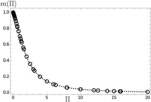
Table 3. m(Π) values obtained by linear regression of the data fitted to Equation (22)(22) $$\frac{F\left(\Pi ,S\right)}{F\left(0,S\right)}\simeq {\left[\frac{F\left(\mathrm{\infty },S\right)}{F\left(0,S\right)}\right]}^{1-m\left(\Pi \right)}.$$(22) .

Π	m(Π)	Π	m(Π)	Π	m(Π)	Π	m(Π)	Π	m(Π)	Π	m(Π)	Π	m(Π)
16	0.01818	12	0.0312	6	0.1066	2	0.4508	1.1	0.6738	0.6	0.8287	0.1	0.9767
15	0.02051	10	0.0435	4	0.2005	1.5	0.5640	1	0.7037	0.4	0.8913	0.01	0.9959
14	0.02336	8	0.0650	3	0.2939	1.2	0.6449	0.8	0.7654	0.2	0.9501	0	1

Computing F(Π,S) based on Equation (21)(21) $$F\left(\Pi ,S\right)\simeq F{\left(0,S\right)}^{m\left(\Pi \right)}F{\left(\mathrm{\infty },S\right)}^{1-m\left(\Pi \right)},$$(21) with the corresponding linear regression values of m(Π) predicts F(Π,S) results in an error of at most ±0.58%. This error is due to inaccuracies in the linear logarithmic relation Equation (22)(22) $$\frac{F\left(\Pi ,S\right)}{F\left(0,S\right)}\simeq {\left[\frac{F\left(\mathrm{\infty },S\right)}{F\left(0,S\right)}\right]}^{1-m\left(\Pi \right)}.$$(22) : ln y = [1 – m(Π)] ln x, and is drastically reducible via the quadratic relation ln y = a₀(Π) + a₁(Π) ln x + a₂(Π) (ln x)²]. This modest ±0.58% error is minimally increased to ±0.60% when inserting the correlation Equation (23)(23) $$m\left(\Pi \right)={\left(1+\hspace{0.17em}\text{exp}\hspace{0.17em}\left[0.101970{\left(\mathit{ln}\Pi \right)}^2+1.474433ln\Pi –0.863914\right]\right)}^{–1}$$(23) for m(Π) in Equation (21)(21) $$F\left(\Pi ,S\right)\simeq F{\left(0,S\right)}^{m\left(\Pi \right)}F{\left(\mathrm{\infty },S\right)}^{1-m\left(\Pi \right)},$$(21) instead of using directly the regression values of m(Π). Equation (23)(23) $$m\left(\Pi \right)={\left(1+\hspace{0.17em}\text{exp}\hspace{0.17em}\left[0.101970{\left(\mathit{ln}\Pi \right)}^2+1.474433ln\Pi –0.863914\right]\right)}^{–1}$$(23) involves a somewhat cumbersome quadratic relation between ln(m⁻¹ – 1) and ln(Π). A linear relation would be equivalent to the more convenient expression (24) $$m\left(\Pi \right)={\left(1+a{\Pi }^b\right)}^{–1}.$$(24)

With a moderate level of optimization we obtain a = 0.4, b = 5/3. Combining Equations (21)(21) $$F\left(\Pi ,S\right)\simeq F{\left(0,S\right)}^{m\left(\Pi \right)}F{\left(\mathrm{\infty },S\right)}^{1-m\left(\Pi \right)},$$(21) and (24)(24) $$m\left(\Pi \right)={\left(1+a{\Pi }^b\right)}^{–1}.$$(24) predict F(Π,S) with a maximal error (±1.8%). This level of approximation is adequate for most filtration/recovery calculations, and drastically outperforms the additive rule Equation (19)(19) $$Z\left(\Pi \right)F_a\left(\Pi ,S\right)\simeq Z_0\left(\Pi \right)F\left(0,S\right)+Z_{\mathrm{\infty }}\left(\Pi \right)F\left(\mathrm{\infty },S\right),$$(19) .

5. Behavior at Π ≫ 1

The two distinguished limits Π ≫ 1 and Π ≪ 1 previously considered theoretically are for all practical purposes condensed in the numerical functions A(S), B(S), included in Table 2. Nonetheless, the region Π ≫ 1 deserves a more detailed theoretical/numerical examination, due to its universal behavior and to clarify the form of the slow upstream (left wing) decay of the diffusive contribution qualitatively suggested by Figure 3b. The analysis of Fernandez de la Mora and Rosner (2019) shows that the behavior in the distinguished limit Π ≫ 1 is universal and is contained in the solution to a reduced PDE free from any parameters (see Equation (25)(25) $$N_{\mathit{zz}}–\sigma N_z=N_{\sigma }, \text{with} N\left(0,\sigma \right)=0 \text{and} N\left(\mathrm{\infty },\sigma \right)=1,$$(25) ). Upon solving this simple PDE once, the information obtained is valid not only at any large (though finite) Π, and for any S < S*, but should apply also to other flow regimes and target geometries. This universal information includes in particular the form of the algebraic decay of the local excess (diffusive) deposition rate, as well as a single numerical quantity Λ (defined in Equation (34)(34) $$\Lambda =\underset{{\sigma }_0\to \mathrm{\infty }}{\mathit{lim}}{\int }_{-{\sigma }_0}^0{\left[N_z\left(\sigma \right)+\sigma \right]}_{z=0}d\sigma +{\int }_0^{\mathrm{\infty }}{\left[N_z\left(\sigma \right)\right]}_{z=0}d\sigma =1.5814$$(34) ) providing the diffusive contribution to the global particle capture (the function A(S)).

The behavior in the region near the critical angle θ* (where the T(θ, Π → ∞, S) plots for Π = ∞ cross the horizontal axis) may be described locally by the parameter-free partial differential equation (25) $$N_{\mathit{zz}}–\sigma N_z=N_{\sigma }, \text{with} N\left(0,\sigma \right)=0 \text{and} N\left(\mathrm{\infty },\sigma \right)=1,$$(25) where z and σ are rescaled forms of the radial and angular variables s and θ near the critical wall tangency point of non-diffusive particle trajectories. Namely, as indicated in Fernandez de la Mora and Rosner (2019), we define the boundary layer-scaled variables corresponding to s and θ – θ* as (26) $$s=1+\delta z,\theta -{\theta }^{*}=\mu \sigma ,$$(26) where the critical angle is given by (27) $$\text{cos}\hspace{0.17em}{\theta }^{*}=\frac{-1+\sqrt{1+16S^2}}{4S}.$$(27)

Since in the limiting case Π ≫ 1 the scaling parameters δ, μ are expected to be small, to a first approximation we substitute s by 1 and θ by θ* in (Equation (6)(6) $${\Pi }^{-3}{N}_{\mathit{ss}}+s^2\left(\frac{1}{2}c\mathit{os}\theta -S\hspace{0.17em}{\text{sin}}^2\theta \right)N_s-s\mathrm{ }\hspace{0.17em}\text{sin}\hspace{0.17em}\theta {\mathrm{ }N}_{\theta }=0.$$(6) ). On the other hand, since the coefficient of the N_s term in Equation (6)(6) $${\Pi }^{-3}{N}_{\mathit{ss}}+s^2\left(\frac{1}{2}c\mathit{os}\theta -S\hspace{0.17em}{\text{sin}}^2\theta \right)N_s-s\mathrm{ }\hspace{0.17em}\text{sin}\hspace{0.17em}\theta {\mathrm{ }N}_{\theta }=0.$$(6) vanishes at θ = θ*, we retain the next order correction, which is proportional to (θ - θ*). Thus, defining the scaling parameters δ, μ as (28) $$\delta =\frac{\hspace{0.17em}{\text{sin}}^{-2/3}{\theta }^{*}}{{\Pi }^2}{\left(1+16S^2\right)}^{-1/6}\ll 1, \mu =\frac{\hspace{0.17em}{\text{sin}}^{-1/3}{\theta }^{*}}{\Pi }{\left(1+16S^2\right)}^{-1/3}\ll 1$$(28) we find to leading order that Equation (6)(6) $${\Pi }^{-3}{N}_{\mathit{ss}}+s^2\left(\frac{1}{2}c\mathit{os}\theta -S\hspace{0.17em}{\text{sin}}^2\theta \right)N_s-s\mathrm{ }\hspace{0.17em}\text{sin}\hspace{0.17em}\theta {\mathrm{ }N}_{\theta }=0.$$(6) reduces to the universal, parameter-free Equation (25)(25) $$N_{\mathit{zz}}–\sigma N_z=N_{\sigma }, \text{with} N\left(0,\sigma \right)=0 \text{and} N\left(\mathrm{\infty },\sigma \right)=1,$$(25) . Note that for large Π the two boundary layers are thin (i.e., δ, μ ≪ 1), as assumed, thus making the analysis consistent.

The initial condition used to start the integration of Equation (25)(25) $$N_{\mathit{zz}}–\sigma N_z=N_{\sigma }, \text{with} N\left(0,\sigma \right)=0 \text{and} N\left(\mathrm{\infty },\sigma \right)=1,$$(25) is obtained by noticing that the N_σ term on its right-hand side is small at sufficiently large negative values of σ. Ignoring entirely this term, one finds to lowest order (29) $$N_0\left(z\right)=1–e^{\sigma z} \text{for} \sigma \ll -1.$$(29)

The small Ν_σ assumption is indeed justified at large negative σ, where N_ozz = σN_z = –σ²e^σz, while the neglected term N_oσ = –ze^σz. Because z ∼ 1/σ within the region where diffusion is relevant, N_σ is much smaller than the other two by the large factor σ³. To the next order we replace N_σ in Equation (25)(25) $$N_{\mathit{zz}}–\sigma N_z=N_{\sigma }, \text{with} N\left(0,\sigma \right)=0 \text{and} N\left(\mathrm{\infty },\sigma \right)=1,$$(25) by ∂N_o/∂σ = –ze^σz and find the improved upstream concentration (30) $$N_1\left(z\right)=1–e^{\sigma z}\left(1–\frac{z}{{\sigma }^2}+\frac{z^2}{2\sigma }\right).$$(30)

The corresponding wall flux to this approximation is (31) $$N_{1z}\left(0\right)=–\sigma +{\sigma }^{-2},$$(31) exhibiting an algebraic decay as σ^–2. To the next order we replace N_σ in Equation (25)(25) $$N_{\mathit{zz}}–\sigma N_z=N_{\sigma }, \text{with} N\left(0,\sigma \right)=0 \text{and} N\left(\mathrm{\infty },\sigma \right)=1,$$(25) by N_1σ and find: (32) $$N_2\left(z\right)=1–e^{\sigma z}\left(1+\frac{z^2}{2\sigma }+\frac{z^4-8z}{8{\sigma }^2}-\frac{z^3}{{\sigma }^3}+\frac{{4z}^2}{{\sigma }^4}-\frac{8z}{{\sigma }^5}\right);N_{2z}\left(0\right)=–\sigma +\frac{1}{{\sigma }^2}+\frac{8}{{\sigma }^5}.$$(32)

Carrying the process to higher orders results in the addition of an extra term of the form a_n/σ^{3n – 1} at each level of iteration: (33) $$N_z\left(0\right)=–\sigma +{\sigma }^{-2}+8{\sigma }^{-5}+175{\sigma }^{-8}+\dots$$(33)

We therefore confirm analytically that the slow upstream decay of the deposition rate to its pure interception asymptote apparent in Figure 3b is indeed algebraic with a leading term 1/σ².

The numerical solution to Equations (25)(25) $$N_{\mathit{zz}}–\sigma N_z=N_{\sigma }, \text{with} N\left(0,\sigma \right)=0 \text{and} N\left(\mathrm{\infty },\sigma \right)=1,$$(25) and (29)(29) $$N_0\left(z\right)=1–e^{\sigma z} \text{for} \sigma \ll -1.$$(29) also confirms that, once the initial condition N_o(z) is applied at a certain large negative initial σ, the solution remains very close to 1 – e^σz at diminishing σ, as long as |σ| ≫ 1. The local mass transfer coefficient is proportional to the quantity [N_z]_z=0, whose numerical values are represented in Figure 10a as a function of the local angular variable σ.

Figure 10. Universal structure of the local rate of deposition in the corner region at large Π, obtained by solving numerically Equations (25)(25) $$N_{\mathit{zz}}–\sigma N_z=N_{\sigma }, \text{with} N\left(0,\sigma \right)=0 \text{and} N\left(\mathrm{\infty },\sigma \right)=1,$$(25) and (29)(29) $$N_0\left(z\right)=1–e^{\sigma z} \text{for} \sigma \ll -1.$$(29) . (a) Note the exponential decay to the right into the horizontal axis, and the slower algebraic decay on the left into the (dashed) line N_z = –σ. (b) Comparison of the numerical calculation (open circles) and the various levels of the asymptotic forms Equation (33)(33) $$N_z\left(0\right)=–\sigma +{\sigma }^{-2}+8{\sigma }^{-5}+175{\sigma }^{-8}+\dots$$(33) .

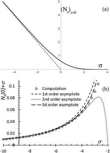
The dashed gray straight line shown in Figure 10a for negative values of σ is the convective particle flux σN (with N = 1), which dominates the collected particle flux at large negative σ. This flux vanishes at the critical point (σ = 0), resulting in a null local convective flux for σ > 0. Diffusion makes a small contribution to the convective flux that rounds off the corner region of the strictly convective prediction. This diffusive correction translates into a slight addition to F(Π, S) with the form given in Equation (17)(17) $$F\left(\Pi ,S\right)\simeq F\left(\mathrm{\infty },S\right)+A\left(S\right){\Pi }^{-2}; \text{for} \Pi \gg 1,$$(17) . We compute the global effect of this correction as the area between the curve in Figure 10a and its two straight line asymptotes: (34) $$\Lambda =\underset{{\sigma }_0\to \mathrm{\infty }}{\mathit{lim}}{\int }_{-{\sigma }_0}^0{\left[N_z\left(\sigma \right)+\sigma \right]}_{z=0}d\sigma +{\int }_0^{\mathrm{\infty }}{\left[N_z\left(\sigma \right)\right]}_{z=0}d\sigma =1.5814$$(34)

The calculation must be carried out carefully because the slow 1/σ² decay of the integrand towards the left results in an even slower convergence of the integral, as 1/σ_o, to its true limit. This important point is fully confirmed by the numerical calculation. This level of accuracy is not provided by Mathematica’s PDE-solver NDSolve command, but is obtained by the pseudospectral orthogonal collocation method, by approximating the dependence of N on variable z, using k Chebyshev polynomials and Chebyshev-Lobatto quadrature, yielding a system of k ordinary differential equations depending on σ. This system of k equations was numerically solved using Mathematica in the domain –σ_o < σ < (1/3)σ_o for increasing values of parameter σ_o between 5 and 40. The numerical difficulty of system Equations (25)(25) $$N_{\mathit{zz}}–\sigma N_z=N_{\sigma }, \text{with} N\left(0,\sigma \right)=0 \text{and} N\left(\mathrm{\infty },\sigma \right)=1,$$(25) and (29)(29) $$N_0\left(z\right)=1–e^{\sigma z} \text{for} \sigma \ll -1.$$(29) increases dramatically as higher values of σ_o are considered. On the one hand, this is because for negative values of σ the solution exhibits a boundary layer with a width proportional to 1/σ_o. On the other hand, for positive values of σ the range of z-values leading to appreciable variations of N increases as ½σ². Actually, the solution of the system Equations (25)(25) $$N_{\mathit{zz}}–\sigma N_z=N_{\sigma }, \text{with} N\left(0,\sigma \right)=0 \text{and} N\left(\mathrm{\infty },\sigma \right)=1,$$(25) and (29)(29) $$N_0\left(z\right)=1–e^{\sigma z} \text{for} \sigma \ll -1.$$(29) for positive values of σ resembles the solution found at σ = 0 advected in the z axis with an increasing velocity given by σ, as can also be expected by inspection of Equation (25)(25) $$N_{\mathit{zz}}–\sigma N_z=N_{\sigma }, \text{with} N\left(0,\sigma \right)=0 \text{and} N\left(\mathrm{\infty },\sigma \right)=1,$$(25) . Consequently, a relatively high number of abscissae for the orthogonal collocation method has been used. With k taking values between k = 30 and k = 100, no significant changes were observed for k > 70. We also tested different values of the maximal z used in the numerical computations (proportional to σ_o² in all cases). In all the cases considered, as soon as the number of abscissae used in the orthogonal collocation method allowed for an accurate description of the boundary layer at small values of z for negative values of σ, the results for Λ agreed with those shown in Equation (34)(34) $$\Lambda =\underset{{\sigma }_0\to \mathrm{\infty }}{\mathit{lim}}{\int }_{-{\sigma }_0}^0{\left[N_z\left(\sigma \right)+\sigma \right]}_{z=0}d\sigma +{\int }_0^{\mathrm{\infty }}{\left[N_z\left(\sigma \right)\right]}_{z=0}d\sigma =1.5814$$(34) . In particular, in all the cases considered the results of the nonlinear fit of Λ to the general model Λ = Λ₀ – aσ_o^-b (computed with Mathematica) produced values of a and b close to 1, in complete agreement with the asymptotic behavior Equation (31)(31) $$N_{1z}\left(0\right)=–\sigma +{\sigma }^{-2},$$(31) (see also Figure 10b). The corresponding asymptote for Λ was in every case 1.5814, indicating that this value is quite accurate.

6. Exploiting particle inertia to improve the recovery of valuable aerosol materials—without “fear of particle rebound”; two specific examples with Π = O(1)

6.1. Important implications of Stk-‘Sub-criticality’

The numerical examples below will demonstrate that the subcritical particle inertial effects we have quantified in Sections 3 and 4 can be exploited to make appreciable gains in fiber filtration performance. Moreover, even when local mainstream particle velocities (often O (1 m/s)) might be large enough to produce particle rebound (in the absence of drag-induced local particle deceleration prior to impact), when the governing Stokes number is sub-critical (i.e., when S < 2.21485) particles which actually arrive at each gas/fiber interface have been decelerated and possess translational velocities associated only with their Brownian motion, lower by more than 2 decades for the examples considered here. Thus, while forward stagnation region inertial enrichment of the suspended particles produces significant improvements in fiber capture performance, aerosol particle impact velocities are well below those expected to produce rebound (as quantified in the vacuum particle-beam experiments of Dahneke 1975), summarized in Friedlander (2000; p 98 ff). This situation is fully consistent with the “perfect capture” approximation at the interception radius a_p + a_f underlying our present mathematical model.

6.2. Two numerical examples

It is instructive to briefly consider two specific examples of the use of these relations to predict the effects of subcritical particle inertia on the expected capture fraction of valuable materials in fiber filtration. Our illustrations both involve the capture of valuable submicron materials (i.e., Pt(s) and Ge(s)) in the simultaneous presence of interception and diffusion, with Π values of O(1). Yet in each case the Reynolds number based on carrier gas velocity and fiber diameter is less than ca. 0.4 (ensuring the accuracy of our Oseen-Stokes local flow field) and the particle Stokes number is less than half of the critical Stokes number for ‘direct impaction’ at the prevailing Reynolds number. In both cases, the carrier gas is considered to be near 300 K and 1 atm, the fiber solid fraction is taken to be 0.04, and the interception parameter R is 0.06 (for 0.6 μm diam. particles captured by a representative 10 μm diam. fiber). Both quoted Stokes numbers are based on the convenient relation: (35) $${\text{Stk}}_p=\frac{{\rho }_p}{{\rho }_g}\frac{C_s\left({\text{Kn}}_p\right)}{9}{R}^2\frac{{\text{Re}}_{t,0}}{1-{\varphi }_t}$$(35) which follows from our definitions, and the assumption of Stokes drag, corrected for carrier gas rarefaction effects using the indicated Cunningham-Millikan slip function (see, also, Rosner and Tandon 2018). Our Stokes-Einstein evaluation of the particle Brownian diffusion coefficient also makes use of C_s(Kn_p), although Kn_f (≡ l_g/a_f) is considered small enough to leave the fiber drag law unaffected [see Equation (A.1) in the Appendix, which addresses the issue of fibrous filter pressure drop]. We focus on our current estimate (using Equation (24)(24) $$m\left(\Pi \right)={\left(1+a{\Pi }^b\right)}^{–1}.$$(24) ) of the factor by which subcritical particle inertia is expected to increase the single fiber capture fraction under the prevailing conditions, i.e., the ratio: (36) $$\frac{{\eta }_{\mathit{cap}}}{{\left({\eta }_{\mathit{cap}}\right)}_{{\text{Stk}}_{\mathit{eff}}=0}}\simeq E\left(S\right)\frac{F\left(\Pi ,S\right)}{F\left(\Pi ,0\right)}$$(36) where, for brevity, S ≡ Stk_eff ≡ Stk_p · C(Re_f).

6.2.1. Pt(s)/N₂(g)

First we consider a dilute suspension of unaggregated platinum particles (ρ_p = 21.45 g/cm³) in nitrogen gas, at a face velocity of 0.3 m/s. For this example we estimate Pe ≈ 0.7 × 10⁵, Re_f ≈ 0.2, Π ≈ 2 and Stk_p ≈ 1.6. At the prevailing value of Stk_p·C(Re_f) ≈ 0.91 the stagnation region (sp) inertial enrichment factor E is near 5.1 (see Table 1). Under these conditions the use of Equation (36)(36) $$\frac{{\eta }_{\mathit{cap}}}{{\left({\eta }_{\mathit{cap}}\right)}_{{\text{Stk}}_{\mathit{eff}}=0}}\simeq E\left(S\right)\frac{F\left(\Pi ,S\right)}{F\left(\Pi ,0\right)}$$(36) along with Table 2, leads to about a 2.0-fold improvement in η_cap/(η_cap)_Stkeff=0. As an immediate consequence, in a depth filter¹ designed to capture, say, 50 pct of the entering Pt (without accounting for subcritical particle inertia), we would now expect a recovery of ca. 75pct, a significant improvement.

6.2.2. Ge(s)/He(g)

Next we consider a dilute suspension of unaggregated germanium particles (ρ_p = 5.32 g/cm³) in helium gas, at a face velocity of 1 m/s. For this example we estimate Pe ≈ 1.66 × 10⁵, Re_f ≈ 0.84 × 10⁻¹, Π ≈ 2.52 and Stk_p ≈ 1.95. At the prevailing value of Stk_p·C(Re_f) ≈ 0.87 the inertial enrichment factor, E, is ca. 4.7. Under these conditions the use of Equation (36)(36) $$\frac{{\eta }_{\mathit{cap}}}{{\left({\eta }_{\mathit{cap}}\right)}_{{\text{Stk}}_{\mathit{eff}}=0}}\simeq E\left(S\right)\frac{F\left(\Pi ,S\right)}{F\left(\Pi ,0\right)}$$(36) along with Table 2 leads to about a 1.9-fold improvement in η_cap/(η_cap)_Stkeff=0. In a depth filter designed to capture, say, 50 pct of the entering Ge (without accounting for subcritical particle inertia), we now would expect a recovery of ca. 73 pct: again a significant improvement.

In comparing this current work with earlier, less general and less convenient estimation methods, we note that previous Brownian dynamics-based numerical simulations of single-fiber capture fractions (e.g., Ramarao et al. [1994], using the Kuwabara ‘cell’ model to account for non-negligible fiber proximity [ϕ_f-] effects, focused on the non-additivity of stochastic and deterministic contributions to the single-fiber capture fraction for a 10-μm diam filament capturing particles with an intrinsic density of ‘only’ 1 g/cc). While most of their numerical results were for much higher Reynolds numbers than considered here, the results of our much earlier 2-fluid continuum “inertial enrichment” approach (Fernandez de la Mora and Rosner 1982) were invoked as a plausible explanation for their numerically observed trends near the condition of “maximum penetration”—i.e., near η_cap,min. We also note that earlier experimental studies of the penetration of a high-efficiency particulate air filter by submicron ‘particles’ of di-ethyl sebacate (ρ_p ≈ 0.96 g/cm³) at U₀ = 0.6 m/s (Gougeon, Boulaud, and Renoux 1996) led these authors to conclude that the systematically lower penetrations they observed for small particles were probably due to what they called the “synergy of diffusion and inertial impaction”—i.e., their neglect of subcritical inertial effects on their estimated capture rate by convective-diffusion. The quantitative inclusion of this phenomenon is now seen to be possible and is fully treated (for cylindrical fibers in low Re cross-flow) in the present work and its immediate predecessor (Fernandez de la Mora and Rosner 2019).

Very recently, Kang et al. (2019) have demonstrated that the Brownian-dynamics computational method can be implemented for low-Re_f two-dimensional flows in cell models of “deep” fibrous filter beds while simultaneously accounting for the distribution of fiber diameters in currently available filters. In this connection, it appears that the ‘factorable’/explicit analytic structure of our present overall result (now summarized in Equation (37)(37) $${\eta }_{\mathit{cap},\mathit{SF}}=2\pi \frac{{\left[C\left(\text{Re}\right)\right]}^{1/3}}{{\left(\text{Pe}\right)}^{2/3}·\left(1+R\right)}\frac{Z\left(\Pi \right)}{\Pi }E\left(S\right)F\left(\Pi ,S\right)$$(37) of Section 6.3) for the single-fiber capture fraction will enable deterministic predictions of this fiber diameter polydispersity effect—at least for single-mode log-normal fiber diameter populations even in the presence of sub-critical particle inertia effects (Rosner and Arias-Zugasti 2020a, 2020b), which will also contain analogous explicit results for the expected consequences of modest aerosol size polydispersity).

6.3. Resulting expression for the multi-mechanism single-fiber capture fraction

While our numerical examples of Section 6.2 focused on the enhancement in capture fraction associated with the presence of subcritical particle inertia, for most applications the absolute value of the resulting single fiber multi-mechanism aerosol capture fraction will be required. Assembling the results presented in Sections 3 and 4 η_cap,SF can be written in the following instructive factorable form: (37) $${\eta }_{\mathit{cap},\mathit{SF}}=2\pi \frac{{\left[C\left(\text{Re}\right)\right]}^{1/3}}{{\left(\text{Pe}\right)}^{2/3}·\left(1+R\right)}\frac{Z\left(\Pi \right)}{\Pi }E\left(S\right)F\left(\Pi ,S\right)$$(37) where the Z(Π) is given by Equation (12)(12) $$Z\left(\Pi \right)={\left[n_s\left(0,\Pi \right)\right]}_{s=1}=\frac{\hspace{0.17em}\text{exp}\hspace{0.17em}\left[-{\Pi }^3/6\right]}{{\int }_1^{\infty }\hspace{0.17em}\text{exp}\hspace{0.17em}\left[-{\left(\Pi s\right)}^3/6\right]ds}=\frac{3^{2/3}\Pi \hspace{0.17em}\text{exp}\hspace{0.17em}\left[-{\Pi }^3/6\right]}{2^{1/3}\Gamma \left(1/3,{\Pi }^3/6\right)},$$(12) . Equation (37)(37) $${\eta }_{\mathit{cap},\mathit{SF}}=2\pi \frac{{\left[C\left(\text{Re}\right)\right]}^{1/3}}{{\left(\text{Pe}\right)}^{2/3}·\left(1+R\right)}\frac{Z\left(\Pi \right)}{\Pi }E\left(S\right)F\left(\Pi ,S\right)$$(37) reveals that subcritical particle inertia appears in both the ‘external’ inertial enrichment function E(S) and the universal bi-variate function: F(Π,S) defined in Section 1, displayed numerically in Section 3, and conveniently represented (to within 1.8 pct) by Equation (24)(24) $$m\left(\Pi \right)={\left(1+a{\Pi }^b\right)}^{–1}.$$(24) in Section 4. This explicit result, Equation (24)(24) $$m\left(\Pi \right)={\left(1+a{\Pi }^b\right)}^{–1}.$$(24) , serving as a local “fundamental solution”, promises to enable much-improved predictions of fibrous filter performance in the foreseeable future.

7. Conclusions

The present study completes the theoretical analysis of Fernandez de la Mora and Rosner (2019) by providing numerical values of the function F(Π,S): i.e., the total aerosol capture rate normalized by the calculable reference rate corresponding to that ‘expected’ if the (accurately predictable) stagnation point particle flux persisted over the entire fiber surface. This enables precise calculations of particle capture to cylinders at modest Reynolds number, due to inertia, diffusion and interception at large effective Peclet number, P, small interception parameter R, and for subcritical effective Stokes numbers, S < S*, where S ≡ C(Re)·Stk and S* = 2.21485. Our principal results and conclusions include:

1. Numerical values (Table 2) of the universal bivariate function F(Π,S) of Fernandez de la Mora and Rosner (2019), providing a thorough description of the behavior of the function F(Π, S) in its full domain (0 < Π < ∞ and 0 < S < S*), including its asymptotes.

2. The use of Table 2 to test the accuracy of the previously used “additive η_cap-approximation” of Lee and Liu (1982), and its generalization to include subcritical particle inertia, given in Equations (19(19) $$Z\left(\Pi \right)F_a\left(\Pi ,S\right)\simeq Z_0\left(\Pi \right)F\left(0,S\right)+Z_{\mathrm{\infty }}\left(\Pi \right)F\left(\mathrm{\infty },S\right),$$(19) and 20)(20a, b) $$Z_0\left(\Pi \right)\equiv \frac{3\Pi }{\sqrt[3]{6}\Gamma \left(1/3\right)}; Z_{\infty }\left(\Pi \right)\equiv \frac{1}{2}{\Pi }^3.$$(20a, b) .

3. The Identification of a convenient power law correlation, given by:

   F(Π,S) ≃ F(0,S)^m(Π) F(∞,S)^1-m(Π), using the exactly known limiting functions F(0,S) and F(∞,S), to represent the function F(Π,S) over its entire Π, S domain. The maximal global error of this representation ranges from only ±0.65% to ±1.8%, depending on the complexity of the auxiliary correlation used to describe the exponent m(Π).

4. We provide a numerical/asymptotic analysis of the universal behavior near the critical tangency point of non-diffusing particles, relevant to the Π ≫ 1 limit. In addition to contributing generally the diffusive correction to the global deposition rate, the study reveals an unusual algebraic (rather than exponential) decay of the diffusive contribution to the particle flux in the region upstream from the critical tangency angle.

5. We illustrate how subcritical particle inertia can be exploited to improve fibrous filter capture fractions “without fear of aerosol particle rebound”—providing (Section 6) two numerical examples involving the recovery of valuable materials (Pt(s) and Ge(s)), as well as relations (Appendix) to anticipate the associated gas pumping requirements.

Nomenclature
m	=	exponent in Equation (21)
a	=	radius (of particle or fiber)
A	=	cross sectional (frontal) area of fibrous filter
C(Re)	=	Oseen-Stokes function C(Re) = [1 + ln(Re−1/2)]−1
CD	=	drag coefficient Equation (A.1)
D	=	particle Brownian diffusivity
E(S)	=	inertial enrichment function of S for forward stagnation line
F(Π, S)	=	function of only Π and S defined by Equations (10)(10) $$T\left(\theta ,\Pi ,S\right)=\frac{{\left[n_s\left(\theta ,\Pi ,S\right)\right]}_{s=1}}{{\left[n_s\left(0,\Pi \right)\right]}_{s=1}}=\frac{e^{-2S\left(1-\hspace{0.17em}\text{cos}\hspace{0.17em}\theta \right)}{\left[N_s\left(\theta ,\Pi ,S\right)\right]}_{s=1}}{Z\left(\Pi \right)};$$(10) and (11)(11) $$F\left(\Pi ,S\right)=\frac{1}{2\pi }{\int }_{\theta }^{2\pi }T\left(\theta ,\Pi ,S\right)d\theta .$$(11) ; see, also, Section 5
n	=	local particle number concentration
N	=	re-normalized local particle number concentration N ≡ n e2S(1 −cosθ) (see Equation (5(5) $$N\equiv n{e}^{2S\left(1-\hspace{0.17em}\text{cos}\hspace{0.17em}\theta \right)}$$(5) ))
P	=	effective Peclet number, P = C(Re)·Pe
Pe	=	Peclet number Pe = 2afU/D = Re·Sc
r	=	cylindrical radius (position variable)
R	=	interception parameter R ≡ ap/af
Re	=	Reynolds number Re = 2af U/νg
s	=	Friedlander’s spatial interception variable s = (r – 1)/R, Equation (2)
S	=	effective Stokes number, S = C(Re)·Stk
Sc	=	Schmidt number for particle diffusion in gas Sc =νg/Dp
Stk	=	Stokes number Stk = τU/af
U	=	fluid velocity at infinity upstream

Greek
ηcap	=	capture fraction for fiber in crossflow (based on frontal area per unit length)
σ	=	angular boundary layer variable, Equation (26)
τ	=	characteristic stopping time for particle in local gas mixture
Π	=	“interception-diffusion similarity parameter,” here Π ≡ R·P1/3
θ	=	polar angle
νg = μg/ρg	=	momentum diffusivity (kinematic viscosity)
χ	=	permeability (of “matte” of fibers); Equation (A.5)(A.5) $$-\Delta p=\mu U_0{L}_f/\chi$$(A.5) .

Subscripts and superscripts
f	=	pertaining to fiber
p	=	pertaining to particles
w	=	evaluated at the wall (r = af)
∞	=	in the upstream gas “far” from the fiber
*	=	identifying the critical value of S or Stk, or the critical (tangent) trajectory
0	=	based on conditions in ambient gas and upstream of a filter
sp	=	stagnation point (Figure 1).

Acronyms
PDE	=	partial differential equation

Notes

1 If particle axial diffusion is negligible compared to axial convection and the overall pressure drop is small compared to the inlet pressure then the  relation between the overall filter capture fraction, η_{cap, SF}, and the single fiber capture fraction η_{cap, SF} will simply be: η_{cap, F} = 1 – exp[–(4/π) φ_f η_{cap, F} L_F/d_f], where  L_F  is the filter “depth” (see, e.g., Friedlander, 2000).

2 Note that for such low Re flows through fiber mattes the conventionally defined bed (matte) permeability “inherits” a weak dependence on both Re_f,0 and ϕ_f via the aforementioned Oseen-Stokes function C(Re).

Appendix: Predictable consequences of increasing the carrier gas “face” velocity: U₀

Inspection of Equations (3), (5)(3) $$\Pi \equiv R{P}^{1/3}$$(3) , and (A.5)(A.5) $$-\Delta p=\mu U_0{L}_f/\chi$$(A.5) governing the evaluation of the parameters Π, Stk, and the Oseen-Stokes function C(Re_f), clearly reveals that (as long as the increased Stk_p remains subcritical) increasing the carrier gas face velocity, U₀, will increase the helpful role of particle inertia in improving aerosol capture performance. However, there remains the question of the extent to which the associated and now predictable gain in (η_cap)_filter will be offset by the also predictable increased pressure drop. The following information should enable this “trade-off” to be examined in each case of interest, while simultaneously satisfying our underlying assumptions.

We recall that in the continuum fluid-dynamic limit the Oseen-Stokes drag coefficient for an infinite length but ‘isolated’ fiber in a low Re_f steady crossflow may be written (Batchelor 1967): (A.1) $$C_D=4\pi ·C\left({\text{Re}}_f\right)/{\text{Re}}_f$$(A.1) where C(Re_f) is the Oseen-Stokes function (Batchelor 1967), re-written here in the form: (A.2) $$C\left({\text{Re}}_f\right)={\left[1+\mathit{ln}\left({\text{Re}}^{-1/2}\right)\right]}^{-1}$$(A.2)

If the fiber is not truly isolated but present in a low solid fraction matte—i.e., with ϕ_f ≪ 1, then (if Re_f,0/(1 – ϕ_f) is less than about 0.4 and the Knudsen number based on a_f is smaller than ca. 0.03), we expect that Equation (A.1) can be generalized to: (A.3) $$C_D=\frac{4\pi \left(1-{\varphi }_f\right)/{\text{Re}}_{f,0}}{1+\mathit{ln}\left[{\left(1-{\varphi }_f\right)}^{1/2}/{\text{Re}}_{f,0}^{1/2}\right]}$$(A.3)

For steady, low Re_f gas flow through such a fiber matte a macroscopic momentum balance can be used to relate the axial force associated with the overall pressure drop to the total drag force experienced by the fibers within the matte. This provides the following useful equation for estimating the effective “permeability” of such a fiber matte—i.e.: (A.4) $$\chi =\frac{1-{\varphi }_f}{{\varphi }_f}·\left(1+\mathit{ln}\left(\frac{{\left(1-{\varphi }_f\right)}^{1/2}}{{\text{Re}}_{f,0}^{1/2}}\right)\right)·\frac{a_f^2}{2}$$(A.4)

From the defining equation for permeability²,² it follows that the expected filter pressure drop, –Δp, can be estimated by simply combining Equation (A.4) with: (A.5) $$-\Delta p=\mu U_0{L}_f/\chi$$(A.5) and the associated pumping power requirement will be the product of this –Δp with the prevailing carrier gas volume flow rate, U₀A.

These relations could be used to evaluate the consequences of increasing U₀ to improve low ϕ_ffibrous filter capture performance due to the often overlooked mechanism of subcritical particle inertia, keeping in mind that, for self-consistency, we should simultaneously satisfy the inequalities underlying our present mathematical model (Section 1), i.e.: (A.6) $${\text{Stk}}_0<\frac{2.21485}{C\left({\text{Re}}_{f,0}\right)}·\left[1-\left(1+\frac{C\left({\text{Re}}_{f,0}\right)}{2}\right)·{\varphi }_f+\dots \right]$$(A.6)

(to leading order in ϕ_f≪ 1) and, say: Re_f,0/(1–ϕ_f) < 0.4 (see, e.g., Kaplun 1957). Our numerical examples (Sections 6.2.1 and 6.2.2), satisfy these conditions.

References

- Batchelor, G. K. 1967. An introduction to fluid dynamics. Cambridge: Cambridge University Press.
- Boyd, J. P. 2000. Chebyshev and Fourier spectral methods. Mineola: Dover.
- Dahneke, B. 1975. Further measurements of the bouncing of small latex spheres. J. Colloid Interface Sci. 51 (1):58–65. doi: 10.1016/0021-9797(75)90083-1.
- Fernandez de la Mora, J., and D. E. Rosner. 2019. Low Reynolds number capture of small particles on cylinders by diffusion, interception, and inertia at subcritical stokes numbers. Aerosol Sci. Technol. 53 (6):647–662. doi: 10.1080/02786826.2019.1587378.
- Fernandez de la Mora, J., and D. E. Rosner. 1982. Effects of inertia on the diffusional deposition of small particle to spheres and cylinders at low Reynolds numbers. J. Fluid Mechan. 125(1):379–395. doi: 10.1017/S0022112082003395.
- Friedlander, S. K. 2000. Smoke, dust and haze: Fundamentals of aerosol dynamics. Oxford: Oxford University Press.
- Gougeon, R., D. Boulaud, and A. Renoux. 1996. Comparison of data from model fiber filters with diffusion, interception and inertial deposition models. Chem. Eng. Commun. 151 (1):19–39. doi: 10.1080/00986449608936539.
- Gottlieb, D., and S. A. Orszag. 1977. Numerical analysis of spectral methods: Theory and applications. Philadelphia: Society for Industrial and Applied Mathematics.
- Hildebrand, F. B. 2013. Introduction to numerical analysis. Mineola: Dover.
- Kang, S., H. Lee, S. C. Kim, D.-R. Chen, and D. Y. H. Pui. 2019. Modeling of fibrous filter media for ultrafine particle filtration. Sep. Purif. Technol. 209 :461–469. doi: 10.1016/j.seppur.2018.07.068.
- Kaplun, S. 1957. Low Reynolds number flow past a circular cylinder. J. Math. Mech. 6:585–593.
- Lee, K. W., and B. Y. H. Liu. 1982. Theoretical study of aerosol filtration by fibrous filters. Aerosol Sci. Technol. 1(2):147–161. doi: 10.1080/02786828208958584.
- Quarteroni, A., and A. Valli. 2008. Numerical approximation of partial differential equations. Berlin: Springer.
- Ramarao, B. V., Tien, C., and S. Mohan. 1994. Calculation of single fiber efficiencies for interception and impaction with superposed Brownian motion. J. Aerosol Sci. 25:295–313. doi: 10.1080/02786828208958584.
- Rosner, D. E., and M. Arias-Zugasti. 2020a. Predicting the aerosol capture characteristics of fibrous filters—I. Tractable method to incorporate log-normal aerosol polydispersity effects with a multi-mechanism semi-analytic single-fiber capture fraction. J. Sep. Purif. Technol.
- Rosner, D. E., and M. Arias-Zugasti. 2020b. Predicting the aerosol capture characteristics of fibrous filters—II. Generalizations of a tractable aerosol PBE approach to include fiber dispersity (wrt diam. and orientation) Using a multi-mechanism, semi-analytic single-fiber capture fraction; comparisons with recent experimental data. J. Sep. Purif. Technol.
- Rosner, D. E., and P. Tandon. 2018. Aggregation and rarefaction effects on particle mass deposition rates by convective-diffusion, thermophoresis or inertial impaction; consequences of ‘momentum shielding. Aerosol Sci. Technol. 52 (3):330–346. doi: 10.1080/02786826.2017.1410095.
- Yeh, H. C. and B. Y. H. Liu. 1974. Aerosol filtration by fibrous filters. J. Aerosol Sci. 5: 191–204 (Theory): 205–7 (Experiments). doi: 10.1016/0021-8502(74)90050-0.