Mixing state evolution of agglomerating particles in an aerosol chamber: Comparison of measurements and particle-resolved simulations

Abstract

This article presents a validation study of the stochastic particle-resolved aerosol model PartMC with experimental data from an aerosol chamber experiment. For the experiment, a scanning mobility particle sizer and a single-particle soot photometer were used to monitor the aerosol mixing state evolution of two initially externally mixed aerosol populations of ammonium sulfate and black carbon particles undergoing agglomeration. We applied an efficient optimization algorithm (ProSRS) to determine several unconstrained simulation parameters and were able to successfully reproduce number concentrations and size distributions of mixed particles that formed by agglomeration. The PartMC modeling approach in conjunction with the optimization procedure provides a tool for detailed comparisons of chamber experiments and modeling, where aerosol mixing state is the focus of investigation.

Copyright © 2019 American Association for Aerosol Research

EDITOR:

• Yannis Drossinos

1. Introduction

Field observations show that individual atmospheric aerosol particles can be a complex mixture of a wide variety of species, such as soluble inorganic salts and acids, insoluble crustal materials, trace metals, and carbonaceous materials (Junge 1952; Moffet et al. 2016; Murphy and Thomson 1997; Prather, Hatch, and Grassian 2008). The diversity in particle composition reflects the various formation processes of atmospheric aerosol particles, and the transformations that they experience during transport in the atmosphere, collectively called “aerosol aging processes.” These include condensation and evaporation of semivolatile substances, multiphase chemical processes on the surface or within the bulk of particles, and coagulation or agglomeration of particles. Here, we refer to coagulation if upon collision the two colliding particles lose their identity (i.e., they coalesce), whereas we refer to agglomeration if the colliding particles retain their identity after the collision.

In describing the complexity in composition of aerosols, the term “mixing state” is frequently used (Winkler 1973). We use this term here to refer to the distribution of the chemical species among the aerosol particles (Riemer et al. 2019; Riemer and West 2013). This concept is often explained by considering the two extremes. On the one hand, an “externally mixed” aerosol has each individual particle consisting of just one species, but with different particles potentially containing different species. On the other hand, an “internally mixed” aerosol has every particle-containing equal proportions of all species, so that all particles have the same composition. In reality, most situations are a state somewhere between those two extremes, neither completely externally nor completely internally mixed (Healy et al. 2014; Ye et al. 2018). The understanding of the aerosol mixing state and its evolution is of crucial importance to assess the aerosol's chemical reactivity (George et al. 2015), cloud condensation nuclei (Farmer, Cappa, and Kreidenweis 2015) and ice nuclei activity (DeMott et al. 2010), and radiative properties (Ravishankara, Rudich, and Wuebbles 2015), which all contribute to the impact of aerosols on climate.

Tools to investigate aerosol mixing state have been developed both on the measurement and the modeling sides. However, to date, few studies have quantitatively compared measured and simulated mixing state information, which is needed for the validation of mixing-state-aware models. One of the challenges to making such comparisons is to find common metrics between the models and the measurement techniques that can form the basis of such a comparison. Some studies have compared model results and field observations on the mixing state of black carbon. For example, Oshima et al. (2009) compared results from a Lagrangian parcel model version of the MADRID-BC model to aircraft data from the PEACE-C campaign that sampled the outflow from Japanese anthropogenic sources with a single-particle soot photometer (SP2) (Moteki et al. 2007). MADRID-BC represents the aerosol population with a two-dimensional bin structure, with one dimension being particle size, and the second dimension being the black carbon mass fraction. The metric used for their comparison was the mass fraction of thickly coated black carbon particles, with “thickly coated” being defined as the particles with a ratio of total diameter to black carbon core diameter larger than two, assuming core-shell morphology. Matsui et al. (2013) compared model simulations from a 2D sectional aerosol model embedded in the regional air quality model WRF-Chem for the region of East Asia with SP2 measurements obtained during the A-FORCE campaign in 2009. They used size-dependent number fractions of black carbon-containing and black carbon-free particles and averaged coating thicknesses as metrics for comparison. Both Oshima et al. (2009) and Matsui et al. (2013) concluded that the simulations were able to reproduce the general features of the observations with respect to their metrics. Their studies also highlighted the importance of black carbon mixing state for accurately predicting aerosol optical properties and cloud condensation nuclei concentrations. While model comparisons to field studies are appealing because they represent the real atmosphere, they are challenging because the mixing states of initial conditions and of emissions are not well quantified.

To our knowledge, a study of mixing state evolution has not yet been performed that quantitatively compares simulation and laboratory data. This is the aim of the current work, which builds on our earlier study by Tian et al. (2017), where we validated the particle resolved aerosol model PartMC (Riemer et al. 2009) with experimental data from a chamber study. However, for Tian et al. (2017) only agglomerating ammonium sulfate particles were considered. Here, we go beyond this and present the first validation of the PartMC model where the aerosol mixing state was evolving. The chamber experiment in this study started with an initially externally mixed aerosol consisting of ammonium sulfate and black carbon particles. During the experiment, the two subpopulations agglomerated and became more and more internally mixed.

The contributions of this study are the quantitative comparison of particle-resolved model output with particle-resolved measurements, and the development of an optimization procedure to constrain the parameters that could not be directly determined experimentally. We base our comparison on the total size distributions, the size distributions of the black carbon-containing components, and the fraction of particles that are mixtures of ammonium sulfate and black carbon particles. As such, this study paves the way for more advanced aerosol chamber-model comparisons where detailed mixing state, particle phase, and particle morphology evolution is the focus.

The manuscript is organized as follows. Section 2 states the governing equation for the evolution of the aerosol in the chamber environment and describes the PartMC simulation algorithm. Section 3 provides details of the chamber experiment, and Section 4 describes the optimization procedure. Sections 5 and 6 present the results and summarize our findings.

2. Model description

2.1. Governing equation for the chamber environment

We consider the evolution of an aerosol population in the chamber that consists of two nonvolatile aerosol species, ammonium sulfate and black carbon, which are introduced into the chamber as external mixtures. We exclude gas-to-particle conversion and aerosol chemistry in our current model framework. The relevant processes are therefore agglomeration, dilution, and wall losses due to diffusion and sedimentation. We assume that the aerosol population in the chamber is well mixed, which justifies a box model approach.

The model formulation is similar to our previous study by Tian et al. (2017), but now includes two different chemical components, ammonium sulfate and black carbon, rather than only one component. We formulate the differential equation governing the time evolution of the aerosol population in the chamber environment in terms of the two-dimensional number distribution $n(\overrightarrow{\mu },t),$ where $\overrightarrow{\mu }=({\mu }_1,{\mu }_2)$ represents the particle composition vector, with the components being the masses of ammonium sulfate (AS) and black carbon (BC). The governing equation is (1) $$\begin{array}{c}\frac{\partial n(\overrightarrow{\mu },t)}{\partial t}=\underset{\text{agglomeration} \text{gain}}{\underbrace{\frac{1}{2}{\int }_0^{{\mu }_1}{\int }_0^{{\mu }_2}K(\overrightarrow{\nu },\overrightarrow{\mu }-\overrightarrow{\nu })n(\overrightarrow{\nu },t)n(\overrightarrow{\mu }-\overrightarrow{\nu },t)d{\nu }_{1}d{\nu }_2}}\\ -\underset{\text{agglomeration} \text{loss}}{\underbrace{{\int }_0^{\infty }{\int }_0^{\infty }K(\overrightarrow{\mu },\overrightarrow{\nu })n(\overrightarrow{\mu },t)n(\overrightarrow{\nu },t)d{\nu }_{1}d{\nu }_2}}\\ +\underset{\text{dilution}}{\underbrace{(n_{\text{fill}}(\overrightarrow{\mu },t)-n(\overrightarrow{\mu },t)){\lambda }_{\text{dil}}(t)}}-(\underset{\text{wall} \text{loss}}{\underbrace{n(\overrightarrow{\mu },t){\alpha }_{\overrightarrow{\mu }}^{\mathrm{D}}(t)+{\alpha }_{\overrightarrow{\mu }}^{\mathrm{S}}(t)}}).\end{array}$$(1)

In Equation (1)(1) $$\begin{array}{c}\frac{\partial n(\overrightarrow{\mu },t)}{\partial t}=\underset{\text{agglomeration} \text{gain}}{\underbrace{\frac{1}{2}{\int }_0^{{\mu }_1}{\int }_0^{{\mu }_2}K(\overrightarrow{\nu },\overrightarrow{\mu }-\overrightarrow{\nu })n(\overrightarrow{\nu },t)n(\overrightarrow{\mu }-\overrightarrow{\nu },t)d{\nu }_{1}d{\nu }_2}}\\ -\underset{\text{agglomeration} \text{loss}}{\underbrace{{\int }_0^{\infty }{\int }_0^{\infty }K(\overrightarrow{\mu },\overrightarrow{\nu })n(\overrightarrow{\mu },t)n(\overrightarrow{\nu },t)d{\nu }_{1}d{\nu }_2}}\\ +\underset{\text{dilution}}{\underbrace{(n_{\text{fill}}(\overrightarrow{\mu },t)-n(\overrightarrow{\mu },t)){\lambda }_{\text{dil}}(t)}}-(\underset{\text{wall} \text{loss}}{\underbrace{n(\overrightarrow{\mu },t){\alpha }_{\overrightarrow{\mu }}^{\mathrm{D}}(t)+{\alpha }_{\overrightarrow{\mu }}^{\mathrm{S}}(t)}}).\end{array}$$(1) , $n(\overrightarrow{\mu },t)$ (${\mathrm{m}}^{-3} {\text{kg}}^{-2}$) is the aerosol number distribution at time t, $K(\overrightarrow{\mu },\overrightarrow{\nu })$ (${\mathrm{m}}^3 {\mathrm{s}}^{-1}$) is the agglomeration coefficient for particles with constituent masses $\overrightarrow{\mu }$ and $\overrightarrow{\nu }, n_{\text{fill}}(\overrightarrow{\mu },t)$ (${\mathrm{m}}^{-3} {\text{kg}}^{-2}$) is the aerosol number distribution of the particles at time t that are introduced into the chamber, ${\lambda }_{\text{dil}}(t)$ (${\mathrm{s}}^{-1}$) is the dilution rate, and ${\alpha }^{\mathrm{D}}(t)$ (${\mathrm{s}}^{-1}$) and ${\alpha }^{\mathrm{S}}(t)$ (${\mathrm{s}}^{-1}$) are the wall loss rate coefficients of diffusion and sedimentation, respectively.

The wall loss treatment (coefficients ${\alpha }_{\overrightarrow{\mu }}^{\mathrm{D}}$ and ${\alpha }_{\overrightarrow{\mu }}^{\mathrm{S}}$) is based on Naumann (2003) and was also used in our previous study by Tian et al. (2017). It provides a formalism of size-dependent wall losses due to particle diffusion and sedimentation. These rates are given by (2) $${\alpha }_{\overrightarrow{\mu }}^{\mathrm{D}}=\frac{D_{\text{diff},\overrightarrow{\mu }}{A}_{\mathrm{D}}}{{\delta }_{\mathrm{D},\overrightarrow{\mu }}{V}_{\mathrm{B}}},$$(2) (3) $${\alpha }_{\overrightarrow{\mu }}^{\mathrm{S}}=\frac{\pi \rho D_{\mathrm{m},\overrightarrow{\mu }}^3 g D_{\text{diff},\overrightarrow{\mu }}{A}_{\mathrm{S}}}{6kT{V}_{\mathrm{B}}}.$$(3)

In Equations (2)(2) $${\alpha }_{\overrightarrow{\mu }}^{\mathrm{D}}=\frac{D_{\text{diff},\overrightarrow{\mu }}{A}_{\mathrm{D}}}{{\delta }_{\mathrm{D},\overrightarrow{\mu }}{V}_{\mathrm{B}}},$$(2) and (3)(3) $${\alpha }_{\overrightarrow{\mu }}^{\mathrm{S}}=\frac{\pi \rho D_{\mathrm{m},\overrightarrow{\mu }}^3 g D_{\text{diff},\overrightarrow{\mu }}{A}_{\mathrm{S}}}{6kT{V}_{\mathrm{B}}}.$$(3) , $D_{\text{diff},\overrightarrow{\mu }}=D_{\text{diff}}(D_{\text{me},\overrightarrow{\mu }})$ (${\mathrm{m}}^2 {\mathrm{s}}^{-1}$) is the diffusion coefficient for particle $\overrightarrow{\mu },$ $D_{\text{me},\overrightarrow{\mu }}$ (m) is the mobility-equivalent diameter of particle $\overrightarrow{\mu }, A_{\mathrm{D}}$ (${\mathrm{m}}^2$) is the diffusional deposition area, ${\delta }_{\mathrm{D},\overrightarrow{\mu }}$ (m) is the diffusional boundary layer thickness for particle $\overrightarrow{\mu },$ and $V_{\mathrm{B}}$ (${\mathrm{m}}^3$) is the volume of the chamber. The thickness ${\delta }_{\mathrm{D},\overrightarrow{\mu }}$ has the following formulation based on Fuchs (1964) and Okuyama et al. (1986), (4) $${\delta }_{\mathrm{D},\overrightarrow{\mu }}=k_{\mathrm{D}}{\left(\frac{D_{\text{diff},\overrightarrow{\mu }}}{D_{\mathrm{u}}}\right)}^a,$$(4) where $k_{\mathrm{D}}$ (m) is a chamber-specific parameter that can vary between different experimental setups. The constant a is a coefficient that was theoretically determined by Fuchs (1964) to be 0.25, and $D_{\mathrm{u}}=1 {\mathrm{m}}^2 {\mathrm{s}}^{-1}$ is the unit diffusion coefficient, which is formally needed to obtain dimensional consistency. In Equation (3)(3) $${\alpha }_{\overrightarrow{\mu }}^{\mathrm{S}}=\frac{\pi \rho D_{\mathrm{m},\overrightarrow{\mu }}^3 g D_{\text{diff},\overrightarrow{\mu }}{A}_{\mathrm{S}}}{6kT{V}_{\mathrm{B}}}.$$(3) , $D_{\mathrm{m},\overrightarrow{\mu }}$ (m) is the mass-equivalent diameter of particle $\overrightarrow{\mu },A_{\mathrm{S}}$ (${\mathrm{m}}^2$) is the sedimentation area of the chamber, ρ is the particle material density ($\text{kg} {\mathrm{m}}^{-3}$), g is the gravitational acceleration ($\mathrm{m} {\mathrm{s}}^{-2}$), k is the Boltzmann constant ($\mathrm{J} {\mathrm{K}}^{-1}$), and T is the temperature (K).

From Tian et al. (2017), we also learned that assuming spherical particle morphology introduces biases in the prediction of the size distributions of agglomerating solid particles. A treatment for fractal particles (Tian et al. 2017) is therefore also used in this article and is summarized in the online supplementary information (SI).

2.2. The PartMC simulation algorithm

PartMC is a stochastic, particle-resolved aerosol box model that solves the governing equation (Equation (1)(1) $$\begin{array}{c}\frac{\partial n(\overrightarrow{\mu },t)}{\partial t}=\underset{\text{agglomeration} \text{gain}}{\underbrace{\frac{1}{2}{\int }_0^{{\mu }_1}{\int }_0^{{\mu }_2}K(\overrightarrow{\nu },\overrightarrow{\mu }-\overrightarrow{\nu })n(\overrightarrow{\nu },t)n(\overrightarrow{\mu }-\overrightarrow{\nu },t)d{\nu }_{1}d{\nu }_2}}\\ -\underset{\text{agglomeration} \text{loss}}{\underbrace{{\int }_0^{\infty }{\int }_0^{\infty }K(\overrightarrow{\mu },\overrightarrow{\nu })n(\overrightarrow{\mu },t)n(\overrightarrow{\nu },t)d{\nu }_{1}d{\nu }_2}}\\ +\underset{\text{dilution}}{\underbrace{(n_{\text{fill}}(\overrightarrow{\mu },t)-n(\overrightarrow{\mu },t)){\lambda }_{\text{dil}}(t)}}-(\underset{\text{wall} \text{loss}}{\underbrace{n(\overrightarrow{\mu },t){\alpha }_{\overrightarrow{\mu }}^{\mathrm{D}}(t)+{\alpha }_{\overrightarrow{\mu }}^{\mathrm{S}}(t)}}).\end{array}$$(1) ). The model resolves the composition of many individual aerosol particles within a well-mixed volume of air. Riemer et al. (2009), DeVille, Riemer, and West (2011), Curtis et al. (2016), and DeVille, Riemer, and West (2019) describe in detail the numerical methods used in PartMC. To summarize, the particle-resolved approach uses a large number of discrete computational particles (10⁴ to 10⁶) to represent the particle population of interest. Each particle is represented by a “composition vector”, which stores the mass of each constituent species within each particle and evolves over the course of a simulation according to various chemical or physical processes. For our study, the relevant processes are Brownian coagulation (agglomeration), dilution and wall losses due to diffusion and sedimentation. They are simulated with a stochastic Monte Carlo approach by generating a realization of a Poisson process. The “weighted flow algorithm” (DeVille, Riemer, and West 2011, 2019) improves the model efficiency and reduces ensemble variance. The code is open-source under the GNU General Public License (GPL) version 2 and can be downloaded at http://lagrange.mechse.illinois.edu/partmc/. We used version 2.4.0 for this work.

We initialized the simulations shown in this article with 10⁴ computational particles. This number changes over the course of the simulation due to particle emissions and particle loss processes, but is kept within the range of $5\times {10}^3$ and $2\times {10}^4$ by “doubling/halving”, which is a common Monte-Carlo particle modeling approach to maintain accuracy (Liffman 1992). If the number of computational particles drops below half of the initial number, the number of computational particles is doubled by duplicating each particle; if the number of computational particles exceeds twice the initial number, then the particle population is down-sampled by a factor of two. These operations correspond to a doubling or halving of the computational volume.

3. Experimental setup

3.1. Setup of chamber measurements

The experiments modeled in this study were a subset of experiments conducted during the third Boston College-Aerodyne Research, Inc. 2012 Black Carbon BC3 study. A detailed account of these experiments was published by Sedlacek et al. (2015). The current work focuses on several experiments that investigated the agglomeration of separate polydisperse distributions of solid black carbon and ammonium sulfate particles. The evolution of these distributions over time, starting from the initial mixing to several hours, were monitored with a condensation particle counter (CPC; TSI model 3775), a scanning mobility particle sizer (SMPS; TSI model 3936), and a single-particle soot photometer (SP2; Droplet Measurement Technology).

The two aerosol distributions were generated using separate atomizers (TSI model 3076), mixed together, diluted with clean air, and dried with an annular diffusion drier packed with molecular sieves (Fisher, 4–8 Mesh) to maintain relative humidity conditions below 40%. The absorbing black carbon (BC) particles were generated from an aqueous suspension of Regal black (Cabot, R400) particles. The non-absorbing ammonium sulfate (AS) particles were generated from an aqueous solution. These aerosols were initially characterized separately to obtain desired number concentrations and mean particle sizes. The ammonium sulfate number distributions were lognormal and had a geometric mean mobility-equivalent diameter of 100 nm and a geometric standard deviation of 1.8, whereas the black carbon number distributions were lognormal with a geometric mean diameter of 200 nm and a geometric standard deviation of 1.6. The agglomeration experiments were conducted in a stainless steel barrel (Skolnik model ST5503). Prior to each experiment, the barrel was purged with particle-free clean air until the background counts were below our detection limits.

The agglomeration experiments were conducted in two stages. The first stage consisted of generating the black carbon and ammonium sulfate particles, mixing the two flows, and streaming the combined aerosol into the barrel for approximately 1 h, filling the barrel to a steady-state concentration. At this point, the barrel was closed to allow the distributions to evolve and agglomerate, initiating the second stage of the experiment. During the second stage, samples were periodically withdrawn from the barrel for measurements, pulling clean air into the barrel through a HEPA filter. When not sampling from the barrel, the instruments were pulling ambient air through a HEPA filter. The samples drawn from the barrel were diluted prior to measurement to minimize coincidence in the SP2 instrument.

3.2. Processing of experimental data

The data reduction and analysis is based on the methodology developed by Sedlacek et al. (2015). As the single-particle soot photometer (SP2) principle of operation has been described in detail elsewhere (e.g., Moteki et al. 2007; Schwarz et al. 2006), we will only highlight the main points here. The SP2 measures the time-dependent scattering and incandescence signals generated by individual BC-containing particles as they travel through a continuous-wave laser beam operating at 1064 nm. As the particle traverses the laser beam, it will scatter light that is recorded by a dedicated detector. Should the particle contain BC, some of the laser energy will be absorbed until the temperature of the BC component is raised to the point of incandescence. The scattering signal provides information on overall particle size and total number concentration of particles (BC-containing and non-BC-containing) whereas the incandescence signal is sensitive to only BC-containing particles. The individual particle incandescence signals are converted to particle mass (obtained via calibration) that can then be converted to an equivalent diameter to yield a BC-specific number or mass distribution. The SP2 community refers to the incandescence BC component as refractory black carbon (rBC). For this article, we will use the term BC for simplicity.

To probe the BC-containing particle morphology, the SP2 takes advantage of the following fact: BC incandescence can only occur for those BC-containing particles for which the associated non-BC material is non-refractory and has been removed. The removal of this non-refractory material occurs when the light-absorbing component of the BC-containing particle (i.e., the BC core) heats up to the point where the non-refractory material is lost via evaporation. This loss of non-refractory material continues until it has been completely removed, leaving a denuded BC particle. Absent any other mechanism to dissipate the spectrally absorbed energy, the now denuded BC particle continues to heat until it reaches its characteristic incandescence temperature (∼3700–4300 K; Schwarz et al. 2006). Given this BC-containing particle lifecycle in the SP2 laser beam, the temporal scattering and incandescence signals observed for individual particles can be used to probe the morphology of these particles.

The temporal behavior of the per-particle scattering peak relative to incandescence peak is known as the lag-time in the SP2 (Moteki et al. 2007). For example, in the bounding limits of a BC particle thickly coated with non-refractory material, the scattering signal maximum can occur earlier than the incandescence maximum (i.e., large positive lag-time) if the non-refractory material fully evaporates prior to incandescence, or later than the incandescence maximum (i.e., large negative lag-time) if some fraction of the non-refractory material is expelled in particulate form from the particle prior to evaporation (Sedlacek et al. 2015). A pure BC particle will exhibit a scattering signal maximum that very closely coincides with the incandescence signal maximum since there is no non-refractory material to burn off.

In this work, we are concerned with mixed AS-BC particles that arise from the agglomeration process. Using the methodology discussed in Sedlacek et al. (2015), the BC-containing particles in our chamber experiment were partitioned into two types: mixed (meaning they contain both AS and BC components) and non-mixed (meaning they contain mainly BC, with the AS component below the detection limit). Apportionment was based on measured lag-times. To account for positive and negative lag-times that can be observed with agglomerated particles, particles with lag-times between $-0.4 \mu$s and $+0.4 \mu$s were classified as being non-mixed while those with lag-times outside this window were labeled as mixed. While it is possible that some mixed particles could generate a lag-time signal that could fall within the non-mixed lag-time window ($-0.4 \mu$s to $0.4 \mu$s), the number of such particles is expected to be small.

4. Determining simulation parameters from experimental data

4.1. Initial condition and emission profiles

The initial condition for the simulation was $n(\overrightarrow{\mu },0)=0.$ Since the experiment was performed in two stages, the filling period during the first 68 min and the sampling period from 68 min onwards, we specified the quantities in the dilution term in Equation (1)(1) $$\begin{array}{c}\frac{\partial n(\overrightarrow{\mu },t)}{\partial t}=\underset{\text{agglomeration} \text{gain}}{\underbrace{\frac{1}{2}{\int }_0^{{\mu }_1}{\int }_0^{{\mu }_2}K(\overrightarrow{\nu },\overrightarrow{\mu }-\overrightarrow{\nu })n(\overrightarrow{\nu },t)n(\overrightarrow{\mu }-\overrightarrow{\nu },t)d{\nu }_{1}d{\nu }_2}}\\ -\underset{\text{agglomeration} \text{loss}}{\underbrace{{\int }_0^{\infty }{\int }_0^{\infty }K(\overrightarrow{\mu },\overrightarrow{\nu })n(\overrightarrow{\mu },t)n(\overrightarrow{\nu },t)d{\nu }_{1}d{\nu }_2}}\\ +\underset{\text{dilution}}{\underbrace{(n_{\text{fill}}(\overrightarrow{\mu },t)-n(\overrightarrow{\mu },t)){\lambda }_{\text{dil}}(t)}}-(\underset{\text{wall} \text{loss}}{\underbrace{n(\overrightarrow{\mu },t){\alpha }_{\overrightarrow{\mu }}^{\mathrm{D}}(t)+{\alpha }_{\overrightarrow{\mu }}^{\mathrm{S}}(t)}}).\end{array}$$(1) as follows: (5) $${\lambda }_{\text{dil}}(t)=\{\begin{array}{cc}\frac{R_{\text{AS}}+R_{\text{BC}}}{V_{\mathrm{B}}},\hfill & t\le 68 \text{min},\hfill \\ \frac{R_{{\text{dil}}_2}}{V_{\mathrm{B}}},\hfill & t>68 \text{min},\hfill \end{array}$$(5) (6) $$n_{\text{fill}}(\overrightarrow{\mu },t)=\{\begin{array}{cc}\frac{R_{\text{AS}}\hspace{0.17em}{n}_{\text{AS}}(\overrightarrow{\mu })+R_{\text{BC}}\hspace{0.17em}{n}_{\text{BC}}(\overrightarrow{\mu })}{R_{\text{AS}}+R_{\text{BC}}},\hfill & t\le 68 \text{min},\hfill \\ 0,\hfill & t>68 \text{min}.\hfill \end{array}$$(6)

The parameters $R_{\text{AS}}$ and $R_{\text{BC}}$ refer to the filling inflow rates of ammonium sulfate particles and black carbon particles, respectively, during the initial filling period, while $R_{{\text{dil}}_2}$ is the outflow rate during the sampling period. The size distributions of the two particle types are specified by (7) $$n_{\text{AS}}(\overrightarrow{\mu })=s_{\mathrm{c},\text{AS}}\hspace{0.17em}{\widehat{n}}_{\text{AS}}(\overrightarrow{\mu }),$$(7) (8) $$n_{\text{BC}}(\overrightarrow{\mu })=s_{\mathrm{c},\text{BC}}\hspace{0.17em}{\widehat{n}}_{\text{BC}}(\overrightarrow{\mu }),$$(8) where ${\widehat{n}}_{\text{AS}}(\overrightarrow{\mu })$ and ${\widehat{n}}_{\text{BC}}(\overrightarrow{\mu })$ are measured diluted inflow distributions of ammonium sulfate and black carbon, respectively, and $s_{\mathrm{c},\text{AS}}$ and $s_{\mathrm{c},\text{BC}}$ are scaling factors to compensate for the dilution. The scaling factors will be determined as part of the optimization procedure in Section 4.2. The inflow distributions $n_{\text{AS}}(\overrightarrow{\mu })$ and $n_{\text{BC}}(\overrightarrow{\mu })$ are shown in Figure 1, using the optimized values of the scaling parameters. Other input parameters are specified in Table 1.

Figure 1. Size distributions of AS (ammonium sulfate) and BC (black carbon) particles that were introduced into the aerosol chamber.

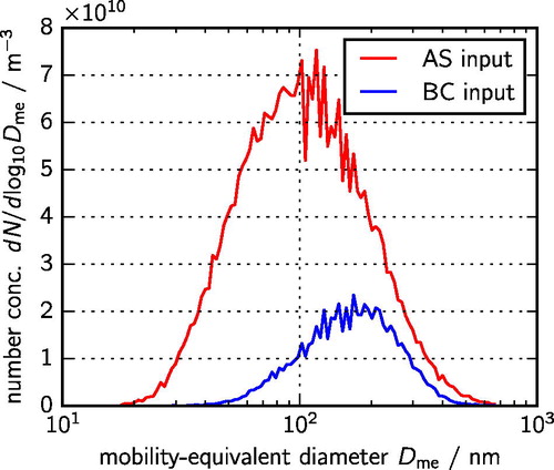
Table 1. Input parameters for chamber experiments.

Parameter	Meaning	Value
$V_{\mathrm{B}}$	Chamber volume	$0.23 {\mathrm{m}}^3$
RH	Relative humidity	10%
T	Temperature	293  K
p	Pressure	10^5 Pa

4.2. Optimization procedure

We identified 12 parameters that need to be prescribed for the PartMC simulations but that are not well constrained from the chamber experiments (see Table 2). We determined these parameters by jointly optimizing them over a predefined domain so that the error between the simulation outputs and the experimental measurements was minimized. We denote the unknown parameters in Table 2 as a 12-dimensional vector $\overrightarrow{x}.$

Table 2. Parameters that were included in the optimization procedure.

Parameter	Meaning	Range	Unit
a	Exponent in diffusional boundary layer thickness	[0.2, 0.3]	1
$k_{\mathrm{D}}$	Prefactor in diffusional boundary layer thickness	[0.02, 0.1]	m
D0	Diameter of primary particles	[6, 200]	nm
f	Volume filling factor	[1.35, 2]	1
$d_{\mathrm{f}}$	Fractal dimension	[1.5, 3]	1
$R_{\text{AS}}$	Filling inflow rate of ammonium sulfate particles	[1, 4]	L/min
$R_{\text{BC}}$	Filling inflow rate for black carbon particles	[1, 4]	L/min
$R_{{\text{dil}}_2}$	Dilution outflow rate during Period 2	[0.5, 4]	L/min
$s_{\mathrm{c},\text{AS}}$	Input scaling factor for ammonium sulfate particles	[100, 400]	1
$s_{\mathrm{c},\text{BC}}$	Input scaling factor for black carbon particles	[100, 400]	1
$s_{\mathrm{c},\text{SMPS}}$	Output scaling factor for SMPS measurements	[100, 400]	1
$s_{\mathrm{c},\text{SP}2}$	Output scaling factor for SP2 measurements	[50, 300]	1

Specifically, for each choice of the 12 parameters in $\overrightarrow{x},$ the PartMC model was simulated with a total simulation time of 220 min, and the outputs were generated every 2 min of simulation. These outputs were then compared to two sets of experimental data: (1) measurement of the total size distribution with an SMPS, and (2) measurement of the black carbon component size distribution with an SP2. The error with respect to the SMPS measurements is given by (9) $${ϵ}_{\text{SMPS}}=\sqrt{\frac{1}{T_1}\sum _{t=1}^{T_1}{({ϵ}_{t,1})}^2},$$(9) where T₁ is the number of SMPS measurement times, and ${ϵ}_{t,1}$ is the relative error of size distributions at time t, defined as (10) $${ϵ}_{t,1}=\sqrt{\frac{\sum _{i=1}^{N_1}{\left(n_{\text{PMC}}^{i,t}-n_{\text{SMPS}}^{i,t}\right)}^2}{\sum _{i=1}^{N_1}{\left(n_{\text{SMPS}}^{i,t}\right)}^2}}.$$(10)

Here $n_{\text{PMC}}^{i,t}$ and $n_{\text{SMPS}}^{i,t}$ represent the number concentration at size bin i and time t for the PartMC simulations and for the SMPS measurements, respectively, and N₁ is the number of bins.

Similarly, the error between the PartMC simulations and the SP2 measurements is given by (11) $${ϵ}_{\text{SP}2}=\sqrt{\frac{1}{T_2}\sum _{t=1}^{T_2}{({ϵ}_{t,2})}^2},\hspace{1em}\text{where} {ϵ}_{t,2}=\sqrt{\frac{\sum _{i=1}^{N_2}{\left(n_{\text{PMC}}^{i,t}-n_{\text{SP}2}^{i,t}\right)}^2}{\sum _{i=1}^{N_2}{\left(n_{\text{SP}2}^{i,t}\right)}^2}}.$$(11)

The measured size distributions from the SMPS and SP2 instruments are given by (12) $$n_{\text{SMPS}}^{i,t}=s_{\mathrm{c},\text{SMPS}} {\widehat{n}}_{\text{SMPS}}^{i,t},$$(12) (13) $$n_{\text{SP}2}^{i,t}=s_{\mathrm{c},\text{SP}2} {\widehat{n}}_{\text{SP}2}^{i,t},$$(13) where ${\widehat{n}}_{\text{SMPS}}^{i,t}$ and ${\widehat{n}}_{\text{SP}2}^{i,t}$ are the measurements after dilution, and $s_{\mathrm{c},\text{SMPS}}$ and $s_{\mathrm{c},\text{SP}2}$ are the dilution scaling factors, so that $n_{\text{SMPS}}^{i,t}$ and $n_{\text{SP}2}^{i,t}$ correspond to the number concentrations in the barrel. The scaling factors are two of the parameters in Table 2 that are determined by the optimization procedure.

The total error ϵ is the root mean square error (RMSE) over the two types of measurements: (14) $$ϵ=\sqrt{\frac{{ϵ}_{\text{SMPS}}^2+{ϵ}_{\text{SP}2}^2}{2}}.$$(14)

Because the simulated number concentrations $n_{\text{PMC}}^{i,t},$ $n_{\text{SMPS}}^{i,t},$ and $n_{\text{SP}2}^{i,t}$ all depend on the value of the parameter vector $\overrightarrow{x},$ the total error ϵ (Equation (14)(14) $$ϵ=\sqrt{\frac{{ϵ}_{\text{SMPS}}^2+{ϵ}_{\text{SP}2}^2}{2}}.$$(14) ) is also dependent on the vector $\overrightarrow{x}.$ Hence, finding the unknown parameters can be formally cast into solving a noisy optimization problem. That is, optimization of the mean of a stochastic (noisy) function: (15) $$\underset{\overrightarrow{x}\in \mathcal{D}}{\mathit{argmin}}E(\overrightarrow{x})={\mathbb{E}}_{\omega }[ϵ(\overrightarrow{x},\omega )].$$(15)

The optimization objective function is the expected error function $E(\overrightarrow{x}),$ which is the average of the total error ϵ defined in Equation (14)(14) $$ϵ=\sqrt{\frac{{ϵ}_{\text{SMPS}}^2+{ϵ}_{\text{SP}2}^2}{2}}.$$(14) . Here the average is taken over repeated runs of the PartMC model with a given parameter vector $\overrightarrow{x}.$ Formally, ω captures the randomness in the PartMC simulations, and $\mathcal{D}$ is the optimization domain given by the parameter ranges in Table 2. Here the optimization objective E is not observed directly but can be estimated via independent random samples of the function ϵ (each sample is a simulation of PartMC). Moreover, the function ϵ is computationally expensive to evaluate since one evaluation requires running a PartMC simulation with some parameter vector $\overrightarrow{x}$ and then computing the error according to Equations (9)(9) $${ϵ}_{\text{SMPS}}=\sqrt{\frac{1}{T_1}\sum _{t=1}^{T_1}{({ϵ}_{t,1})}^2},$$(9) –(14)(14) $$ϵ=\sqrt{\frac{{ϵ}_{\text{SMPS}}^2+{ϵ}_{\text{SP}2}^2}{2}}.$$(14) .

The problem described by Equation (15)(15) $$\underset{\overrightarrow{x}\in \mathcal{D}}{\mathit{argmin}}E(\overrightarrow{x})={\mathbb{E}}_{\omega }[ϵ(\overrightarrow{x},\omega )].$$(15) is a standard simulation optimization problem (Amaran et al. 2016), which we solved using an efficient parallel surrogate optimization algorithm, known as ProSRS¹ (Shou and West 2019). ProSRS is an iterative algorithm where in each iteration, a radial basis function (RBF) model that approximates the objective function is first constructed using available evaluations, and then a new set of point(s) is proposed based on the RBF model. Compared to other optimization methods (Anderson and Ferris 2001; Contal et al. 2013; Elster and Neumaier 1995; González et al. 2016; Shah and Ghahramani 2015; Snoek, Larochelle, and Adams 2012), ProSRS has three appealing characteristics. First, it allows parallel evaluations of the expensive function ϵ (Equation (14)(14) $$ϵ=\sqrt{\frac{{ϵ}_{\text{SMPS}}^2+{ϵ}_{\text{SP}2}^2}{2}}.$$(14) ) during optimization. Second, it is a global optimization algorithm with asymptotic guarantees that is known to work well for complex, multimodal functions. Third, the algorithm is efficient to run, so that the computational overhead of executing it is typically negligible relative to the expensive function evaluations.

For the SMPS measurements, the number of times T₁ (Equation (9)(9) $${ϵ}_{\text{SMPS}}=\sqrt{\frac{1}{T_1}\sum _{t=1}^{T_1}{({ϵ}_{t,1})}^2},$$(9) ) is 66 and the number of size bins N₁ (Equation (10)(10) $${ϵ}_{t,1}=\sqrt{\frac{\sum _{i=1}^{N_1}{\left(n_{\text{PMC}}^{i,t}-n_{\text{SMPS}}^{i,t}\right)}^2}{\sum _{i=1}^{N_1}{\left(n_{\text{SMPS}}^{i,t}\right)}^2}}.$$(10) ) is 106. For the SP2 measurements, the number of times T₂ and the number of bins N₂ are 54 and 200, respectively (see Equation (11)(11) $${ϵ}_{\text{SP}2}=\sqrt{\frac{1}{T_2}\sum _{t=1}^{T_2}{({ϵ}_{t,2})}^2},\hspace{1em}\text{where} {ϵ}_{t,2}=\sqrt{\frac{\sum _{i=1}^{N_2}{\left(n_{\text{PMC}}^{i,t}-n_{\text{SP}2}^{i,t}\right)}^2}{\sum _{i=1}^{N_2}{\left(n_{\text{SP}2}^{i,t}\right)}^2}}.$$(11) ). As a result, the optimization problem consists of fitting a total of $T_1{N}_1+T_2{N}_2=66\times 106+54\times$ 200 = 17,796 data points with the 12 parameters listed in Table 2. The parameters affect the time evolution of the modeled distributions in diverse, nonlinear, size-dependent ways, so it is plausible that the relatively small number of parameters has little risk of overfitting. This nonlinear dependence of the time-evolving aerosol state on the parameters is due both to direct nonlinearities with respect to many of the parameters (e.g., the wall loss exponent a) and to the fact that agglomeration rates scale nonlinearly with concentration and are size-dependent. This means that even parameters such as inflow rates, which linearly affect the number of particles added to the chamber, actually produce size-dependent and nonlinear changes in the size distributions. To better understand these effects, we computed sensitivities of the fit with respect to the parameters, as described below.

We ran the ProSRS algorithm with 800 iterations on 32-core XE nodes of Blue Waters² with the algorithm configured to use all the cores of a node (i.e., ProSRS proposed 32 different values of $\overrightarrow{x}$ for parallel evaluations at each iteration). The per-iteration time-cost of running ProSRS was approximately 3 s, which was about 1–2 orders of magnitude lower than that of evaluating the error function ε (one evaluation took about 100 s).

Running ProSRS yielded a total of $800\times 32=$ 25,600 evaluations of the error function ϵ (Equation (14)(14) $$ϵ=\sqrt{\frac{{ϵ}_{\text{SMPS}}^2+{ϵ}_{\text{SP}2}^2}{2}}.$$(14) ). The next step was to select, from all the evaluated vectors $\overrightarrow{x},$ the one with the lowest expected error E (Equation (15)(15) $$\underset{\overrightarrow{x}\in \mathcal{D}}{\mathit{argmin}}E(\overrightarrow{x})={\mathbb{E}}_{\omega }[ϵ(\overrightarrow{x},\omega )].$$(15) ). Since the expected error E is unknown and we have only one noisy evaluation of it (i.e., one evaluation of function ϵ) per vector $\overrightarrow{x},$ selecting the true best vector is not trivial. For this, we used a simple selection procedure based on Monte Carlo estimates.

This selection procedure consists of three steps. First, from the 25,600 evaluations, we chose the 100 vectors with the lowest ϵ values. Second, for each candidate vector $\overrightarrow{x},$ we performed ten independent evaluations of function ϵ and used the average of these ten evaluations as the mean estimate of the expected error $E(\overrightarrow{x}).$ Finally, the candidate with the lowest mean estimate was reported as the optimum, and its value is shown in the second column of Table 3. The mean estimate of the error for this optimum is 0.1559. Figure 2 illustrates the entire optimization workflow from defining a problem, running ProSRS, to finally selecting the best vector.

Figure 2. Optimization workflow for determining the vector $\overrightarrow{x}$ of unknown parameters listed in Table 2 for the PartMC simulation. We first defined a minimization problem (Equation (15)(15) $$\underset{\overrightarrow{x}\in \mathcal{D}}{\mathit{argmin}}E(\overrightarrow{x})={\mathbb{E}}_{\omega }[ϵ(\overrightarrow{x},\omega )].$$(15) ), then ran an iterative surrogate-based optimization algorithm (ProSRS), and finally selected the best vector from the ProSRS candidate vectors. RBF stands for radial basis function.

Table 3. Optimization results.

Parameter	Unit	Optimal value	Confidence interval (CI)	Rel. CI mag. (%)
a	1	0.230	[0.203, 0.254]	22.2
$k_{\mathrm{D}}$	m	0.086	[0.051, 0.097]	52.8
D0	nm	74	[66, 84]	26.0
$d_{\mathrm{f}}$	1	2.15	$[2.02,2.37]$	16.3
f	1	1.41	[1.35, 1.76]	28.8
$R_{\text{AS}}$	L/min	1.70	[1.51, 1.93]	25.0
$R_{\text{BC}}$	L/min	1.70	[1.51, 1.93]	25.0
$R_{{\text{dil}}_2}$	L/min	1.08	[0.944, 1.14]	18.1
$s_{\mathrm{c},\text{AS}}$	1	271	[231, 297]	22.8
$s_{\mathrm{c},\text{BC}}$	1	284	[255, 312]	20.2
$s_{\mathrm{c},\text{SMPS}}$	1	253	[216, 287]	27.8
$s_{\mathrm{c},\text{SP}2}$	1	217	[192, 236]	20.3

When formulating the dilution term in Equation (1)(1) $$\begin{array}{c}\frac{\partial n(\overrightarrow{\mu },t)}{\partial t}=\underset{\text{agglomeration} \text{gain}}{\underbrace{\frac{1}{2}{\int }_0^{{\mu }_1}{\int }_0^{{\mu }_2}K(\overrightarrow{\nu },\overrightarrow{\mu }-\overrightarrow{\nu })n(\overrightarrow{\nu },t)n(\overrightarrow{\mu }-\overrightarrow{\nu },t)d{\nu }_{1}d{\nu }_2}}\\ -\underset{\text{agglomeration} \text{loss}}{\underbrace{{\int }_0^{\infty }{\int }_0^{\infty }K(\overrightarrow{\mu },\overrightarrow{\nu })n(\overrightarrow{\mu },t)n(\overrightarrow{\nu },t)d{\nu }_{1}d{\nu }_2}}\\ +\underset{\text{dilution}}{\underbrace{(n_{\text{fill}}(\overrightarrow{\mu },t)-n(\overrightarrow{\mu },t)){\lambda }_{\text{dil}}(t)}}-(\underset{\text{wall} \text{loss}}{\underbrace{n(\overrightarrow{\mu },t){\alpha }_{\overrightarrow{\mu }}^{\mathrm{D}}(t)+{\alpha }_{\overrightarrow{\mu }}^{\mathrm{S}}(t)}}).\end{array}$$(1) , it can be shown that the four parameters $R_{\text{AS}},R_{\text{BC}},$ $s_{\mathrm{c},\text{AS}},s_{\mathrm{c},\text{BC}}$ only appear in three distinct combinations, so there is one unconstrained degree of freedom. Specifically, for $t\le 68 \text{min},$ substituting Equations (5)–(8) into the dilution term of Equation (1)(1) $$\begin{array}{c}\frac{\partial n(\overrightarrow{\mu },t)}{\partial t}=\underset{\text{agglomeration} \text{gain}}{\underbrace{\frac{1}{2}{\int }_0^{{\mu }_1}{\int }_0^{{\mu }_2}K(\overrightarrow{\nu },\overrightarrow{\mu }-\overrightarrow{\nu })n(\overrightarrow{\nu },t)n(\overrightarrow{\mu }-\overrightarrow{\nu },t)d{\nu }_{1}d{\nu }_2}}\\ -\underset{\text{agglomeration} \text{loss}}{\underbrace{{\int }_0^{\infty }{\int }_0^{\infty }K(\overrightarrow{\mu },\overrightarrow{\nu })n(\overrightarrow{\mu },t)n(\overrightarrow{\nu },t)d{\nu }_{1}d{\nu }_2}}\\ +\underset{\text{dilution}}{\underbrace{(n_{\text{fill}}(\overrightarrow{\mu },t)-n(\overrightarrow{\mu },t)){\lambda }_{\text{dil}}(t)}}-(\underset{\text{wall} \text{loss}}{\underbrace{n(\overrightarrow{\mu },t){\alpha }_{\overrightarrow{\mu }}^{\mathrm{D}}(t)+{\alpha }_{\overrightarrow{\mu }}^{\mathrm{S}}(t)}}).\end{array}$$(1) gives (16) $$\begin{array}{l}(n_{\text{fill}}(\overrightarrow{\mu },t)-n(\overrightarrow{\mu },t)){\lambda }_{\text{dil}}(t)\\ =\frac{1}{V_{\mathrm{B}}}(\underset{C_1}{\underbrace{R_{\text{AS}} s_{\mathrm{c},\text{AS}}}}{\widehat{n}}_{\text{AS}}(\overrightarrow{\mu },t)+\underset{C_2}{\underbrace{R_{\text{BC}} s_{\mathrm{c},\text{BC}}}}{\widehat{n}}_{\text{BC}}(\overrightarrow{\mu },t)-\underset{C_3}{\underbrace{(R_{\text{AS}}+R_{\text{BC}})}}n(\overrightarrow{\mu },t)).\end{array}$$(16)

Here we see that we really only have three free parameters (C₁, C₂, C₃) rather than four ($R_{\text{AS}},R_{\text{BC}},$ $s_{\mathrm{c},\text{AS}},s_{\mathrm{c},\text{BC}}$). Intuitively, this redundancy arises because we have over-parameterized the model by including separate parameters for the inflow rates ($R_{\text{AS}},R_{\text{BC}}$) and the input scaling factors ($s_{\mathrm{c},\text{AS}},s_{\mathrm{c},\text{BC}}$). In reality, we only have three independent quantities that are physically meaningful (two inflow concentrations and one net outflow rate). We could have chosen to write the original model equations with only three parameters (the C₁, C₂, C₃ parameters above) but we feel that this would make the model less clear.

To remove the redundancy in our choice of parameters, we can add an extra restriction on the four parameter values. We arbitrarily chose $R_{\text{AS}}=R_{\text{BC}}$ (equal inflow rates) as this extra restriction, because it is simple and numerically well-conditioned. Note that this modeling choice does not alter the optimization procedure or model simulations in any way, because any difference in the actual experimental inflow rates will be compensated for in the model by changes to the input scaling factors. We performed the optimization in the full 12-dimensional parameter space but then mapped the parameters to preserve C₁, C₂, C₃ and to satisfy the arbitrary additional restriction $R_{\text{AS}}=R_{\text{BC}}.$ This additional restriction removed the extra unconstrained degree of freedom. Concretely, given parameters $(R_{\text{AS}}^{\prime },R_{\text{BC}}^{\prime },s_{\mathrm{c},\text{AS}}^{\prime },s_{\mathrm{c},\text{BC}}^{\prime }),$ we mapped them to (17) $$R_{\text{AS}}=R_{\text{BC}}=\frac{1}{2}(R_{\text{AS}}^{\prime }+R_{\text{BC}}^{\prime }),$$(17) (18) $$s_{\mathrm{c},\text{AS}}=\frac{2R_{\text{AS}}^{\prime }}{R_{\text{AS}}^{\prime }+R_{\text{BC}}^{\prime }}{s}_{\mathrm{c},\text{AS}}^{\prime },$$(18) (19) $$s_{\mathrm{c},\text{BC}}=\frac{2R_{\text{BC}}^{\prime }}{R_{\text{AS}}^{\prime }+R_{\text{BC}}^{\prime }}{s}_{\mathrm{c},\text{BC}}^{\prime },$$(19) which preserves C₁, C₂, C₃ and has equal inflow rates.

We conducted a sensitivity analysis for the optimum parameter vector, and the results are summarized in terms of the confidence interval (CI) shown in the last two columns of Table 3. These CIs can be viewed as a quantitative measure of how sensitive the objective function E (Equation (15)(15) $$\underset{\overrightarrow{x}\in \mathcal{D}}{\mathit{argmin}}E(\overrightarrow{x})={\mathbb{E}}_{\omega }[ϵ(\overrightarrow{x},\omega )].$$(15) ) is to perturbations in the parameter vector $\overrightarrow{x}$ around the optimum. To compute the CIs, we first estimated the standard deviation of the noise in the error function ϵ using the aforementioned independent evaluations of the 100 candidate vectors. The standard deviation was estimated to be about 0.005. We then found all the vectors, among the candidate vectors, for which the mean estimate of the error was within one standard deviation above the best value (i.e., within the interval $[0.1559,0.1559+0.005]$). If we denote the collection of these within-one-standard-deviation vectors as the set $\mathcal{A},$ then the CI lower limit $\overrightarrow{l}$ is defined as ${\overrightarrow{l}}_i={\text{min}}_{\overrightarrow{x}\in \mathcal{A}}{\overrightarrow{x}}_i$ ($i=1,2,\dots ,12$), where subscript i denotes the $i^{\text{th}}$ dimension of a vector. Similarly, the CI upper limit $\overrightarrow{u}$ is given by ${\overrightarrow{u}}_i={\text{max}}_{\overrightarrow{x}\in \mathcal{A}}{\overrightarrow{x}}_i.$ The relative CI magnitude $\overrightarrow{m}$ is computed relative to the optimum ${\overrightarrow{x}}_{\text{opt}}$ (the second column of Table 3) as ${\overrightarrow{m}}_i=({\overrightarrow{u}}_i-{\overrightarrow{l}}_i)/{({\overrightarrow{x}}_{\text{opt}})}_i.$ From the above definitions, we can see that a smaller relative CI magnitude in a dimension implies the objective function is more sensitive to the change of values in that dimension around the optimum.

5. Results and discussion

In this section, we will first discuss the values of the optimal parameters as listed in Table 3 that carry physical meaning (a, $k_{\mathrm{D}},\hspace{0.17em}{d}_{\mathrm{f}},$ D₀, f), and then present the results of the evolution of measured and simulated aerosol populations in the barrel. From the results for the optimal parameters (Table 3), we learn the following. Our value for the wall loss parameter, a = 0.230, CI $[0.203,0.254],$ is consistent with the theoretical value of 0.25 that was derived by Fuchs (1964). The coefficient $k_{\mathrm{D}}$ is proportional to the laminar boundary layer thickness used in the wall loss parameterization and can vary between different experimental setups (Bunz and Dlugi 1991). Our estimate for $k_{\mathrm{D}},\hspace{0.17em}{k}_{\mathrm{D}}=0.086$ m, CI $[0.051,0.097]$, is similar to our previous results described in Tian et al. (2017), where we determined a value of 0.06 m, and also similar to the results by van de Vate and ten Brink (1980) who determined a value of 0.048 m as their best fit.

The parameter D₀ represents the diameter of the primary particles that comprise the fractal aggregates formed by agglomeration. As shown in Figure 1, the primary particles (ammonium sulfate and black carbon) are polydisperse and they have already undergone some unknown amount of agglomeration during the process of formation and injection into the chamber. The use of one constant D₀ parameter for both species is a simplification. Our optimal value for this parameter, $D_0=74$ nm, CI $[66,84]$ nm, is therefore to be interpreted as an “effective diameter” and represents an aspect of the model that should be improved in the future.

Our optimal fractal dimension, $d_{\mathrm{f}}=2.15,$ CI $[2.02,2.37],$ is clearly below the value of 3 for spherical particles, indicating that the aggregates that are formed by agglomeration cannot be assumed to be spherical. However, it is larger than the value of 1.78 predicted by diffusion-limited cluster-cluster aggregation (DLCA) theory (Sorensen 2011). This can be explained by the fact that the aggregates only contain a small number of primary particles, and therefore our fitted value does not represent the “true fractal dimension” but needs to be adjusted for the small-N case (Tian et al. 2017).

As described in Sorensen (2011), in this case, the scaling of the mobility-equivalent diameter $D_{\text{me}}$ can be written as (20) $$D_{\text{me}}=\beta D_{\text{geo}}\propto \beta N^{1/{\widehat{d}}_{\mathrm{f}}}\propto N^{-0.13}{N}^{1/{\widehat{d}}_{\mathrm{f}}},$$(20) where ${\widehat{d}}_{\mathrm{f}}$ is the true fractal dimension, $D_{\text{geo}}$ is the geometric diameter, and N is the number of primary particles. As detailed in SI Equation (S-3), we are using the Naumann (2003) relationship (21) $$D_{\text{me}}=h_{\text{KR}}{D}_{\text{geo}}=h_{\text{KR}}{D}_0{\left(\mathit{fN}\right)}^{1/d_{\mathrm{f}}}\propto N^{1/d_{\mathrm{f}}}.$$(21)

Importantly, the Kirkwood-Riseman ratio $h_{\text{KR}}$ does not depend on N, and so we see that in the small-N case the parameter $d_{\mathrm{f}}$ in the Naumann (2003) model that we use is in fact the mass-mobility scaling exponent $D_{\text{ms}}$ described by Sorensen (2011), which is defined by the relationship $D_{\text{me}}\propto N^{1/D_{\text{ms}}}.$ Note that $D_{\text{ms}}$ is denoted $D_{\mathrm{m}}$ in Sorensen (2011). From our optimization procedure, we obtain the value $d_{\mathrm{f}}=2.1,$ hence (22) $$D_{\text{me}}\propto N^{1/d_{\mathrm{f}}}=N^{0.43}$$(22) (23) $$\propto N^{-0.13}{N}^{1/{\widehat{d}}_{\mathrm{f}}},$$(23) and matching these two expressions allows us to compute that the true fractal dimension implied by our model is ${\widehat{d}}_{\mathrm{f}}=1.68.$ This is close to the theoretically expected value of $1.78\pm 0.1$ for DLCA processes (Sorensen 2011). Similar to the parameter D₀, we consider the fractal dimension derived here as an “effective” parameter applied to all particles over the entire duration of the experiment, and future model improvement should include a refinement of this assumption.

The volume filling factor f accounts for the fact that the spherical primary particles can occupy only as much as 74% of the available volume, in which case f would be 1.35. Larger values of f correspond to less dense packing. Our optimal value of 1.41 corresponds to the primary particles occupying about 70% of the volume, a value that is plausible, but that we cannot confirm with independent measurements.

Figures 3 and 4 both show the experimental data that were used to perform the optimization as described in Section 4.2 as red lines, and the corresponding model output as blue lines. Figure 3 shows the total size distributions at 10, 50, 108, and 192 min, while Figure 4 shows the distributions of the black carbon aerosol component at the same times. The simulated results were obtained using the optimal parameter values as listed in Table 3. In these and later figures, the simulation results are the means of ten PartMC simulations and the lighter-colored bands around the simulation curves represent the standard deviations of the mean estimates. In later figures, the standard deviation is visually negligible and is not plotted.

Figure 3. Simulated (blue line) and measured (red line) total size distributions at 10, 50, 108, and 192 min. These size distributions were used in the optimization procedure described in Section 4.2. The green line shows the simulated size distribution of mixed particles, defined here as the particles containing between 10 and 90% ammonium sulfate.

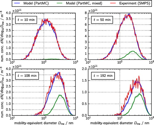
Figure 4. Simulated (blue line) and measured (red line) size distributions of black carbon particle components at 10, 50, 108, and 192 min. These size distributions were used in the optimization procedure described in Section 4.2.

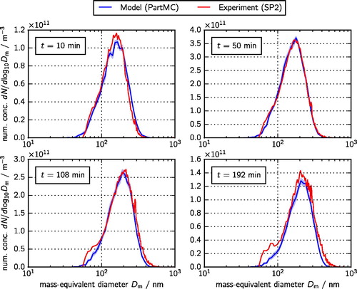
For all times, the simulated size distributions follow the measured distributions well, which is expected for a successful optimization exercise. We observe a growth of the particles due to agglomeration as the mode of the distribution moves from 100 nm to 400 nm (Figure 3). The distribution of black carbon component sizes evolves much less (Figure 4), with the mode increasing from about 150 nm to 200 nm. This is expected because the relatively low abundance of black carbon (Figure 1) means that agglomeration events between pairs of particles that both contain black carbon are relatively less frequent.

Figure 3 also shows the simulated size distributions of “mixed particles” as green lines with the light green band representing the standard deviation of the mean estimate based on ten PartMC simulations. We categorized as mixed particles those with ammonium sulfate mass fractions between 10% and 90%. As expected, over the course of the simulation, the abundance of mixed particles increases.

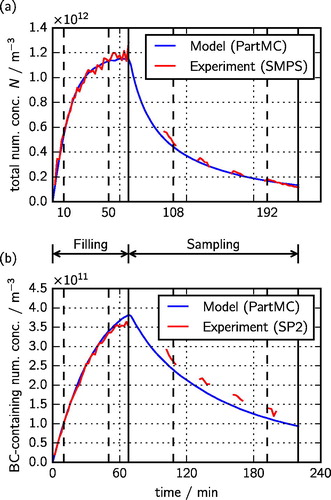
Figures 5a and b show the time series of simulated and measured total number concentrations, and of the number concentrations of black carbon particles, respectively. The gaps in the measured time series during the sampling period are due to the fact that sampling occurred through a filter. We can clearly distinguish the filling period, when the number concentration increases, from the sampling period, when the number concentration decreases due to agglomeration, dilution, and wall losses. The measured and modeled values match well over the entire record for the total number concentration, while the simulation somewhat underpredicted the number concentration of the black carbon-containing particles during the sampling phase.

Figure 5. Time series of (a) total particle number concentration and (b) number concentration of black carbon-containing particles in the barrel over the course of the experiment. The simulated results of the optimized PartMC model are shown in blue, and the experimental results are shown in red. The vertical broken lines indicate the times shown in Figures 3, 4, and 7, while the vertical solid lines indicate the ends of the filling and sampling periods.

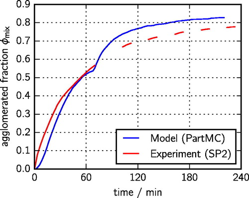
Figure 6 shows the time series of the agglomerated fraction ${\varphi }_{\text{mix}},$ which we defined as (24) $${\varphi }_{\text{mix}}=\frac{N_{\text{mix}}}{N_{\text{BC}}+N_{\text{mix}}},$$(24) where $N_{\text{mix}}$ is the number concentration of mixed particles, and $N_{\text{BC}}$ is the number concentration of pure black carbon particles. As before, for the simulated results, we consider a particle as “mixed” when the mass fraction of the second species is at least 10%. For this figure, we only included particles between 200 nm and 450 nm to match the size range that the SP2 captures. The simulated time series of ${\varphi }_{\text{mix}}$ follows the observed time series well. This comparison provides an independent validation of our modeling approach since the observational data were not used in the optimization procedure.

Figure 6. Simulated (blue line) and measured (red line) fraction of black carbon-containing particles that have undergone agglomeration. These values were not directly used in the optimization procedure, and so the agreement between simulated and measured values is a validation of the model.

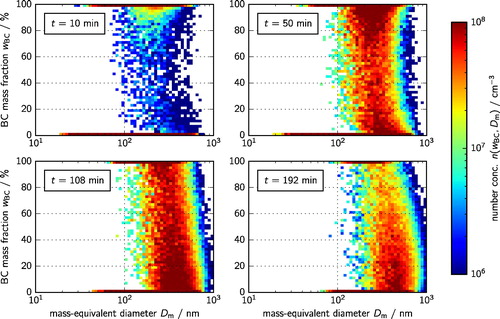
Figure 7 displays the simulated two-dimensional size distribution $n(w_{\text{BC}},D_{\mathrm{m}}),$ which is defined as the derivative $n(w_{\text{BC}},D_{\mathrm{m}})={\partial }^{2}N(w_{\text{BC}},D_{\mathrm{m}})/(\partial w_{\text{BC}}\partial {\hspace{0.17em}\text{log}\hspace{0.17em}}_{10}{D}_{\mathrm{m}})$ of the two-dimensional cumulative number distribution $N(w_{\text{BC}},D_{\mathrm{m}})$ in terms of black carbon mass fraction $w_{\text{BC}}$ and particle mass-equivalent diameter $D_{\mathrm{m}}.$ Since we only consider two species, this figure represents the full mixing state of the population. At t = 10 min, early during the filling period, mixed particles had already formed throughout the entire range of mass fractions, resulting in a rather complicated aerosol mixing state that cannot be easily estimated. This figure confirms that it was necessary to perform the simulation from the beginning of the filling period (rather than starting after the filling), as this was the only time when the initial conditions were known.

Figure 7. Two-dimensional simulated size distributions $n(w_{\text{BC}},D_{\mathrm{m}})$ at 10, 50, 108, and 192 min.

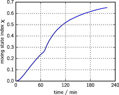
The evolution of the mixing state can be more precisely quantified by the mixing state index χ (Riemer and West 2013), which ranges in general from 0 for completely external mixtures to 100% for completely internal mixtures. It is given by the affine ratio of the diversity metrics $D_{\alpha }$ and $D_{\gamma }:$ (25) $$\chi =\frac{D_{\alpha }-1}{D_{\gamma }-1}.$$(25)

The diversity metrics, in turn, are defined as follows. First, the per-particle mixing entropies H_i need to be calculated based on the per-particle species mass fractions. These values are then averaged over the entire population to give $H_{\alpha },$ and finally the average particle species diversity $D_{\alpha }.$ For our system of two species (AS and BC), these can be written as (26) $$H_i=-w_{\text{BC}}^i\hspace{0.17em}\text{ln}\hspace{0.17em}{w}_{\text{BC}}^i-\left(1-w_{\text{BC}}^i\right)\hspace{0.17em}\text{ln}\hspace{0.17em}\left(1-w_{\text{BC}}^i\right),$$(26) (27) $$H_{\alpha }=\frac{1}{\sum _i{m}_i}\sum _i{m}_i{H}_i,$$(27) (28) $$D_{\alpha }=\hspace{0.17em}\text{exp}\hspace{0.17em}\left(H_{\alpha }\right),$$(28) where $w_{\text{BC}}^i$ is the mass fraction of BC in particle i, and m_i is the mass of particle i. Second, the bulk population diversity is given by (29) $$H_{\gamma }=-w_{\text{BC}}^{\text{bulk}}\hspace{0.17em}\text{ln}\hspace{0.17em}{w}_{\text{BC}}^{\text{bulk}}-\left(1-w_{\text{BC}}^{\text{bulk}}\right)\hspace{0.17em}\text{ln}\hspace{0.17em}\left(1-w_{\text{BC}}^{\text{bulk}}\right),$$(29) (30) $$D_{\gamma }=\hspace{0.17em}\text{exp}\hspace{0.17em}\left(H_{\gamma }\right),$$(30) where $w_{\text{BC}}^{\text{bulk}}$ is the bulk mass fraction of BC. Since $H_{\alpha }$ is obtained by a mass-weighted average of the per-particle mixing entropies H_i (Equation (27)(27) $$H_{\alpha }=\frac{1}{\sum _i{m}_i}\sum _i{m}_i{H}_i,$$(27) ), the mixing state index χ reflects the mixing state of the particles that constitute most of the aerosol mass of the population. For example, a large value of χ indicates that most of the mass resides in mixed particles. In our experiment, the mixing state index increased monotonically from 0 at the start to 65% at the end of the simulation, as shown in Figure 8, representing a partially internally mixed population, consistent with Figure 7.

Figure 8. Time series of the simulated mixing state index χ for the optimized PartMC model.

6. Conclusions

For the first time, the particle-resolved model PartMC was validated with experimental data where the aerosol mixing state evolved as two initially externally mixed particle populations underwent agglomeration in an aerosol chamber. The evolution of the particle population was monitored with an SMPS and an SP2 instrument over the course of several hours. The model simulations included agglomeration, dilution and wall losses, and accounted for the non-spherical shape of the aggregates. We applied an efficient optimization algorithm (ProSRS) to determine several unconstrained parameters using the total size distributions and the size distributions of the black carbon particle components. Both PartMC and ProSRS are publicly available at https://github.com/compdyn/PartMC and https://github.com/compdyn/ProSRS, respectively.

Using the set of optimized parameters, the model was able to fit well the time evolution of total number concentrations. The number of concentration of black carbon-containing particles was somewhat underpredicted. The simulated number fraction of mixed particles, which was not explicitly fit, matched the observations well. The mixing state of the population, quantified by the mixing state index χ, evolved quickly as soon as the particles entered the chamber, moving from a completely external mixture to a partially internal mixture.

This work provides the foundation for more sophisticated studies that might include additional aerosol processes, such as gas-particle partitioning or particle restructuring, or studies that quantify mixing state impacts on population-integrated quantities, such as total absorption. Adding condensable vapors to the experimental setup increases the challenge of representing the dynamic evolution of the population for several reasons, including accounting for wall losses of vapors and the multi-generation of reaction products (Sunol, Charan, and Seinfeld 2018), and competition effects between particles of different sizes or compositions. Particle-resolved modeling is particularly appropriate for these kinds of complex scenarios as it can accurately account for these inter-particle competitive effects. The ProSRS algorithm used in this work can be applied to estimate unconstrained parameters related to these processes, e.g., parameters related to wall losses, production rates of secondary species, or morphology parameters. For these purposes, it would be useful to obtain additional observational constraints, for example scanning electron microscopy images to quantify the evolution of particle composition and morphology. An area of future model improvement is the representation of particle morphology including the treatment of fractal particles, especially when condensable vapors are involved (Heinson, Liu, and Chakrabarty 2017).

Additional information

Funding

We acknowledge DOE-ASR funding from grants DE-SC0011771, DE-SC0019192, DE-SC0012704, DE-SC0006980, and DE-SC0011935. M. W. acknowledges support from NSF CMMI 11-50490. N. R. acknowledges funding from NSF AGS 1254428. This research is part of the Blue Waters sustained-petascale computing project, which is supported by the National Science Foundation (awards OCI-0725070 and ACI-1238993) and the state of Illinois. Blue Waters is a joint effort of the University of Illinois at Urbana-Champaign and its National Center for Supercomputing Applications.

Notes

1 ProSRS code is publicly available at https://github.com/compdyn/ProSRS.

2 Blue Waters: https://bluewaters.ncsa.illinois.edu.

References

- Amaran, S., N. V. Sahinidis, B. Sharda, and S. J. Bury. 2016. Simulation optimization: a review of algorithms and applications. Ann Oper Res. 240 (1):351–380. doi: 10.1007/s10479-015-2019-x.
- Anderson, E. J., and M. C. Ferris. 2001. A direct search algorithm for optimization with noisy function evaluations. SIAM J Optim. 11 (3):837–857. doi: 10.1137/S1052623496312848.
- Bunz, H., and R. Dlugi. 1991. Numerical studies on the behavior of aerosols in smog chambers. J. Aerosol. Sci. 22 (4):441–465. doi: 10.1016/0021-8502(91)90004-2.
- Contal, E., D. Buffoni, A. Robicquet, and N. Vayatis. 2013. Parallel Gaussian process optimization with upper confidence bound and pure exploration. In Joint European Conference on Machine Learning and Knowledge Discovery in Databases, ed. H. Blockeel, K. Kersting, S. Nijssen, and F. Železný, 225–240. Berlin, Heidelberg: Springer.
- Curtis, J., M. Michelotti, N. Riemer, M. Heath, and M. West. 2016. Accelerated simulation of stochastic particle removal processes in particle-resolved aerosol models. J. Comput. Phys. 322:21–32. doi: 10.1016/j.jcp.2016.06.029.
- DeMott, P. J., A. J. Prenni, X. Liu, S. M. Kreidenweis, M. D. Petters, C. H. Twohy, M. Richardson, T. Eidhammer, and D. Rogers. 2010. Predicting global atmospheric ice nuclei distributions and their impacts on climate. Proc. Natl. Acad. Sci. U.S.A. 107 (25):11217–11222. doi: 10.1073/pnas.0910818107.
- DeVille, R., N. Riemer, and M. West. 2011. Weighted flow algorithms (WFA) for stochastic particle coagulation. J. Comput. Phys. 230 (23):8427–8451. doi: 10.1016/j.jcp.2011.07.027.
- DeVille, L., N. Riemer, and M. West. 2019. Convergence of a generalized weighted flow algorithm for stochastic particle coagulation. J. Comput. Dyn. 6:69–94.
- Elster, C., and A. Neumaier. 1995. A grid algorithm for bound constrained optimization of noisy functions. IMA J Numer. Anal. 15 (4):585–608. doi: 10.1093/imanum/15.4.585.
- Farmer, D. K., C. D. Cappa, and S. M. Kreidenweis. 2015. Atmospheric processes and their controlling influence on cloud condensation nuclei activity. Chem. Rev. 115 (10):4199–4217. doi: 10.1021/cr5006292.
- Fuchs, N. A. 1964. Mechanics of aerosols. New York: Pergamon.
- George, C., M. Ammann, B. D mann, D. Donaldson, and S. A. Nizkorodov. 2015. Heterogeneous photochemistry in the atmosphere. Chem. Rev. 115 (10):4218–4258. doi: 10.1021/cr500648z.
- González, J., Z. Dai, P. Hennig, and N. Lawrence. 2016. Batch Bayesian optimization via local penalization. In Proceedings of the 19th International Conference on Artificial Intelligence and Statistics, Vol. 51, ed. A. Gretton and C. C. Robert, 648–657. Cadiz, Spain: Proceedings of Machine Learning Research.
- Healy, R. M., N. Riemer, J. C. Wenger, M. Murphy, M. West, L. Poulain, A. Wiedensohler, I. P. O’Connor, E. McGillicuddy, J. R. Sodeau, and G. J. Evans. 2014. Single particle diversity and mixing state measurements. Atmos. Chem. Phys. 14 (12):6289–6299. doi: 10.5194/acp-14-6289-2014.
- Heinson, W. R., P. Liu, and R. K. Chakrabarty. 2017. Fractal scaling of coated soot aggregates. Aerosol Sci. Technol. 51 (1):12–19. doi: 10.1080/02786826.2016.1249786.
- Junge, C. E. 1952. Die konstitution des atmosphärischen aerosols. Ann. Met. 5:1–55.
- Liffman, K. 1992. A direct simulation Monte-Carlo method for cluster coagulation. J. Comput. Phys. 100 (1):116–127. doi: 10.1016/0021-9991(92)90314-O.
- Matsui, H., M. Koike, Y. Kondo, N. Moteki, J. D. Fast, and R. A. Zaveri. 2013. Development and validation of a black carbon mixing state resolved three-dimensional model: Aging processes and radiative impact. J. Geophys. Res. 118:2304–2326. doi: 10.1029/2012JD018446.
- Moffet, R. C., R. E. O’Brien, P. A. Alpert, S. T. Kelly, D. Q. Pham, M. K. Gilles, D. A. Knopf, and A. Laskin. 2016. Morphology and mixing of black carbon particles collected in Central California during the CARES field study. Atmos. Chem. Phys. 16 (22):14515–14525. doi: 10.5194/acp-16-14515-2016.
- Moteki, N., Y. Kondo, Y. Miyazaki, N. Takegawa, Y. Komazaki, G. Kurata, T. Shirai, D. Blake, T. Miyakawa, and M. Koike. 2007. Evolution of mixing state of black carbon particles: Aircraft measurements over the western pacific in March 2004. Geophys. Res. Lett. 34:L11803.
- Murphy, D., and D. Thomson. 1997. Chemical composition of single aerosol particles at Idaho hill: Negative ion measurements. J. Geophys. Res. 102 (D5):6353–6368. doi: 10.1029/96JD00859.
- Naumann, K. 2003. COSIMA – A computer program simulating the dynamics of fractal aerosols. J. Aerosol Sci. 34 (10):1371–1397. doi: 10.1016/S0021-8502(03)00367-7.
- Okuyama, K., Y. Kousaka, S. Yamamoto, and T. Hosokawa. 1986. Particle loss of aerosols with particle diameters between 6 and 2000 nm in stirred tank. J. Colloid Interface Sci. 110 (1):214–223. doi: 10.1016/0021-9797(86)90370-X.
- Oshima, N., M. Koike, Y. Zhang, and Y. Kondo. 2009. Aging of black carbon in outflow from anthropogenic sources using a mixing state resolved model: 2. Aerosol optical properties and cloud condensation nuclei activities. J. Geophys. Res. 114:D18202. doi: 10.1029/2008JD011681.
- Prather, K. A., C. D. Hatch, and V. H. Grassian. 2008. Analysis of atmospheric aerosols. Annu Rev Anal Chem. 1:485–514. doi: 10.1146/annurev.anchem.1.031207.113030.
- Ravishankara, A., Y. Rudich, and D. Wuebbles. 2015. Physical chemistry of climate metrics. Chem. Rev. 115 (10):3682–3703. doi: 10.1021/acs.chemrev.5b00010.
- Riemer, N., A. P. Ault, R. L. Craig, J. H. Curtis, and M. West. 2019. Aerosol mixing state: Measurements, modeling, and impacts. Rev. Geophys. 57:187–249. doi: 10.1029/2018RG000615.
- Riemer, N., and M. West. 2013. Quantifying aerosol mixing state with entropy and diversity measures. Atmos. Chem. Phys. 13 (22):11423–11439. doi: 10.5194/acp-13-11423-2013.
- Riemer, N., M. West, R. A. Zaveri, and R. C. Easter. 2009. Simulating the evolution of soot mixing state with a particle-resolved aerosol model. J. Geophys. Res. 114:D09202. doi: 10.1029/2008JD011073.
- Schwarz, J. P., R. S. Gao, D. W. Fahey, D. S. Thomson, L. A. Watts, J. C. Wilson, J. M. Reeves, M. Darbeheshti, D. G. Baumgardner, G. L. Kok, S. H. Chung, M. Schulz, J. Hendricks, A. Lauer, B. Kärcher, J. G. Slowik, K. H. Rosenlof, T. L. Thompson, A. O. Langford, M. Loewenstein, and K. C. Aikin. 2006. Single-particle measurements of midlatitude black carbon and light-scattering aerosols from the boundary layer to the lower stratosphere. J. Geophys. Res. 111 (D16):D16207. doi: 10.1029/2006JD007076.
- Sedlacek, A. J., E. R. Lewis, T. B. Onasch, A. T. Lambe, and P. Davidovits. 2015. Investigation of refractory black carbon-containing particle morphologies using the single-particle soot photometer (SP2). Aerosol Sci. Technol. 49 (10):872–885. doi: 10.1080/02786826.2015.1074978.
- Shah, A., and Z. Ghahramani. 2015. Parallel predictive entropy search for batch global optimization of expensive objective functions. In Advances in neural information processing systems, ed. C. Cortes, N. D. Lawrence, D. D. Lee, M. Sugiyama, and R. Garnett, 3330–3338. Curran Associates, Inc.
- Shou, C., and M. West. 2019. A tree-based radial basis function method for noisy parallel surrogate optimization. arXiv e-prints. https://arxiv.org/abs/1908.07980.
- Snoek, J., H. Larochelle, and R. P. Adams. 2012. Practical Bayesian optimization of machine learning algorithms. In Advances in neural information processing systems, ed. F. Pereira, C. J. C. Burges, L. Bottou, and K. Q. Weinberger, 2951–2959. Curran Associates, Inc.
- Sorensen, C. M. 2011. The mobility of fractal aggregates: A review. Aerosol Sci. Technol. 45 (7):765–779. doi: 10.1080/02786826.2011.560909.
- Sunol, A., S. Charan, and J. Seinfeld. 2018. Computational simulation of the dynamics of secondary organic aerosol formation in an environmental chamber. Aerosol Sci. Technol. 52 (4):470–482. doi: 10.1080/02786826.2018.1427209.
- Tian, J., B. Brem, M. West, T. Bond, M. Rood, and N. Riemer. 2017. Simulating aerosol chamber experiments with the particle-resolved aerosol model PartMC. Aerosol Sci. Technol. 51 (7):856–867. doi: 10.1080/02786826.2017.1311988.
- van de Vate, J. F., and H. M. ten Brink. 1980. The boundary layer for diffusive aerosol deposition onto walls. Proceedings of the CSNI Specialists Meeting on Nuclear Aerosols in Reactor Safety, Gatlinburg, TN, USA, 162–170.
- Winkler, P. 1973. The growth of atmospheric aerosol particles as a function of the relative relative humidity—II. an improved concept of mixed nuclei. J. Aerosol Sci. 4 (5):373–387. doi: 10.1016/0021-8502(73)90027-X.
- Ye, Q., P. Gu, H. Z. Li, E. S. Robinson, E. Lipsky, C. Kaltsonoudis, A. K. Y. Lee, J. S. Apte, A. L. Robinson, R. C. Sullivan, A. A. Presto, and N. M. Donahue. 2018. Spatial variability of sources and mixing state of atmospheric particles in a metropolitan area. Environ. Sci. Technol. 52 (12):6807–6815. doi: 10.1021/acs.est8b01011.