Transport of indoor aerosols to hidden interior spaces

Abstract

Most studies on indoor aerosols have focused on the open spaces within buildings that are visible to occupants, while the hidden spaces in buildings receive much less attention. Indeed, little is known about the extent to which indoor aerosols are transported into closets, cabinets and drawers. Aerosols deposited in these hidden spaces serve as a reservoir for particulate matter with the potential for resuspension within homes. To investigate aerosol transport to indoor hidden spaces, a series of experiments were conducted in a full-scale test house. Specifically, aerosols released indoors were tracked using a fluorometric method and the air circulation between the open and hidden spaces were measured using tracer gas techniques. The results show that momentum-driven flow caused by fan operation had a negligible impact on the overall air circulation between rooms and hidden spaces. Rather, the circulation was driven primarily by buoyancy forces caused by temperature differences between the hidden spaces and adjacent rooms. In the well-controlled, three-bedroom two-bathroom test house used in this study, aerosols released indoors dispersed and deposited across the open spaces and even within closets with closed doors. For more sealed spaces like closed drawers within closed cabinets, the air circulation rates between the adjacent room and hidden space were substantially lower and a much lower fraction of the indoor aerosols deposited in these areas. Nevertheless, the results indicate that at least one percent of the indoor aerosol source penetrated into the most remote indoor hidden spaces.

Copyright © 2019 American Association for Aerosol Research

Introduction

Hidden spaces in buildings include crawl spaces, wall cavities, cabinets, closets, drawers and other areas that are not directly visible, accessible and/or maintained. In contrast to the open areas of homes and other buildings, relatively little is known about how indoor aerosols move between spaces visible to occupants and spaces are hidden from view. Given that particles harbor microorganisms (Barberan et al. 2015; Hospodsky et al. 2015; Weikl et al. 2016), semi-volatile organic compounds (Dodson et al. 2012; Kolarik, Naydenov, et al. 2008; Langer et al. 2016; Naumova et al. 2002; Stapleton et al. 2009; Wilford et al. 2005), heavy metals (Glorennec et al. 2012; Rasmussen et al. 2018; Satsangi et al. 2014; Turner and Simmonds 2006; Wang et al. 2018) and other contaminants of concern to human health, it is important to quantify the extent to which aerosols released indoors deposit into reservoirs within hidden spaces. Indeed, human exposure to indoor aerosols has been shown to cause inflammation, cytotoxicity and lung injury (Happo et al. 2013; Long et al. 2001; Monn and Becker 1999; Ormstad 2000; Shao et al. 2007). In addition, exposure to particulate matter (PM) of biological origin is associated with infectious disease transmission as well as allergic and non-allergic respiratory illnesses (Doekes et al. 2005; Douwes et al. 2003; Srikanth, Sudharsanam, and Steinberg 2008).

Particles in indoor environments have different origins, including cooking or smoking (Hussein et al. 2006; Long, Suh, and Koutrakis 2000; Miller and Nazaroff 2001; Nazaroff 2004; Ogulei, Hopke, and Wallace 2006; Wainman et al. 2000; Wallace 1996), infiltration (El Orch, Stephens, and Waring 2014; Hoek et al. 2008), occupant shedding or resuspension from floors and interior surfaces (Boor, Siegel, and Novoselac 2013b; Boor et al. 2015; Ferro, Kopperud, and Hildemann 2004; Hospodsky et al. 2012; Long, Suh, and Koutrakis 2000; Nazaroff 2004; Spilak et al. 2014; Täubel et al. 2009), or aerosolization from showers or other similar sources (Adams et al. 2017; Estrada-Perez et al. 2018; Prussin and Marr 2015). The movement of these particles indoors depends on the distribution of airflows which can be driven by the heating, ventilation and air conditioning (HVAC) fan and/or by buoyancy flows resulting from temperature differences between rooms, exterior walls and indoor air. Previous research by Rim and Novoselac (2008) demonstrated that both fan and buoyancy driven flows are sufficient to disperse airborne aerosols throughout a room and an entire house. Although the initial peak concentration after aerosol injection differs for these two driving forces, the ultimate particle dispersion is similar regardless of what is driving the airflow and particle dispersion. Other studies have found that for aerosols released indoors, the presence of closed doors reduces the subsequent aerosol concentration in the non-source room; however, for most homes with open doors, aerosol concentrations eventually become uniform across rooms after the emissions have stopped (Miller and Nazaroff 2001; Ott, Klepeis, and Switzer 2003).

Indoor aerosol fate studies generally focus on particle movement and deposition in the open spaces within buildings that are visible to occupants (Ferro, Kopperud, and Hildemann 2004; Ju and Spengler 1981; Miller and Nazaroff 2001; Ott, Klepeis, and Switzer 2003; Thatcher et al. 2002). Most work that has investigated aerosol transport to hidden spaces has focused on bioaerosol transport to and from crawl spaces, wall cavities and HVAC system components. For instance, previous studies have examined the transport of bioaerosols emitted from crawl spaces, including fungal spores and molds (Bok, Hallenberg, and Åberg 2009; Johansson, Svensson, and Ekstrand-Tobin 2013; Pessi et al. 2002). These studies have demonstrated that the movement of spores from crawl spaces to the occupied space is driven by pressure differences (Airaksinen, Kurnitski, et al. 2004; Airaksinen, Pasanen, et al. 2004), and that relatively simple engineering solutions – such as depressurizing the crawl space – can prevent this transport (Hayashi et al. 2014; Keskikuru et al. 2018). For other hidden spaces such as cavities in the building envelope, the transport of mold spores from these cavities to the indoor environment is heavily dependent on the wall construction type (Rao et al. 2006). The surfaces of heat exchangers in HVAC systems are also a major source of airborne bacteria, viruses and fungi in the built environment (Prussin and Marr 2015), and deposition and resuspension of particles and fungal spores in cooling coils and ventilation ducts can contribute to indoor air quality problems (Boor, Siegel, and Novoselac 2013a; Krauter, Biermann, and Larsen 2005; Siegel and Walker 2001; Waring and Siegel 2008; Wu et al. 2016; Zhou, Zhao, and Tan 2011). Furthermore, a few studies have examined the movement of air within closets to determine the emissions of volatile organic compounds from closets (Chang and Krebs 1992; Guerrero and Corsi 2012) but little is known about what is driving this air movement and how it affects aerosol transport to the interior of closets.

While previous studies confirm that understanding and maintaining hidden spaces are important for ensuring good indoor air quality in occupied spaces, interior hidden spaces such as closets, cabinets and drawers have received much less attention, specifically with respect to particle penetration and deposition. These indoor spaces may contribute to human exposure as bioaerosols and other particulate-bound pollutants can potentially penetrate and deposit on clothing, dishware or food stored within. Generally, those hidden spaces are considered “safe” from aerosol contamination and thus the objective of the current study is to investigate if this assumption is justifiable or if such hidden spaces serve as a sink for aerosol pollutants. Specifically, this study investigates the transport of air and aerosols between rooms and adjacent hidden spaces such as closets, cabinets and drawers. To this end, the airflow exchange and the fate of traceable particles were monitored in a full-scale test house to determine the penetration and deposition of PM into hidden spaces as a function of environmental conditions including spatial temperature differences as well as fan-driven air motion.

Methodology

Experimental design

In order to evaluate the transport and fate of aerosols in a realistic residential environment, a series of seven aerosol and tracer gas (carbon dioxide – CO₂) injection experiments (M1–M7, Table 1) were completed within an unoccupied three-bedroom/two-bath test house (UTest House, Figure 1) in Austin, TX. During these experiments, the movement and deposition of the injected fluorescent particles as well as the movement of the CO₂ simultaneously injected in the control room were monitored as a function of time and position within the test house. Six additional tracer gas experiments were completed to measure the circulation of air between indoor hidden spaces and surrounding rooms as described in Table 1 (HAC 1–HAC 6). The temperature profiles in the rooms as well as the temperature within the hidden spaces were also measured to assess whether they influenced the movement of particles and tracer gas. Finally, to confirm whether or not momentum from the central air conditioning system penetrated into hidden interior spaces, the air velocities (AV) within three hidden spaces (closets, cabinets and drawers) were examined in more detail in Experiments AV 1 and AV 2. The conditions associated with each of the 15 experiments conducted in the UTest House are summarized in Table 1.

Figure 1. Layout of the test house (UTest House) used in this study. The injection point (dot [orange]) was located at a height of 1.4 m next to the window in the control room. The sample collection points (dots [white]) are also identified, as well as the outdoor air inlet (arrows [blue]) and the window opening (rectangle [blue]) in the master bedroom.

Table 1. Summary of experimental conditions for the UTest House experiments.

Exp.	Ventilation conditions		ACH of outdoor air^a (h^−1)		Surface sampling locations for fluorescent particles (FP)^e
	AHU^b	DMV System^c	Set by AHU or DMV	Measured at MR^d
M1–M7: aerosol and tracer gas injection experiments to evaluate the transport and fate of aerosols; CO2 injected for experiments M2–M7; temperature measured in all seven experiments; airborne particle concentration measured in experiments M3–M7
M1	Off	On	1	NA^f	CR, SR, KR, MR, MB
M2	Off	On	1	1.0	CR, SR, KR, MR, MB
M3	Off	On	1	1.1	CR, SR, KR, MR, MB, SRC, MRC, MBC
M4	Off	Off	0	0.5	CR, SR, KR, MR, MB, SRC, MRC, MBC, KRD 1, KRD 2
M5	Off	On	1	0.9	CR, SR, KR, MR, MB, SRC, MRC, MBC, KRD 1, KRD 2
M6	Off	On	1	1.2	CR, SR, KR, MR, MB, SRC, MRC, MBC, KRD 1, KRD 2
M7	Off	Off	0	0.3	CR, SR, KR, MR, MB, SRC, MRC, MBC, KRD 1, KRD 2
HAC 1–HAC 6: additional tracer gas experiments to measure the air circulation between indoor hidden spaces and surrounding rooms; CO2 and temperature measured in all six experiments
HAC 1	Off	On	1	Not applicable	No particles were injected
HAC 2	Off	On	1
HAC 3	Off	On	1
HAC 4	Off	Off	0
HAC 5	Off	Off	0
HAC 6	Off	Off	0
AV 1–AV 2: air velocity experiments to confirm whether momentum from the central air conditioning system penetrated into hidden interior spaces including closets and drawers; only the air velocities within closets and drawers were measured
AV 1	Off	Off	0	Not applicable	No particles were injected
AV 2	On	Off	8

^a ACH: air change rate per hour.

^b AHU: air handling unit.

^c DMV: dedicated mechanical ventilation.

^d Measured ACH in MR (master bedroom) are different than AHU or DMV setpoint due to the variable infiltration rate.

^e Locations: CR – control room, SR – second bedroom, KR – kitchen, MR – master bedroom, MB – master bathroom, SRC – second bedroom closet, MRC – master bedroom closet, MBC – master bathroom cabinet, KRD 1 – kitchen drawer 1, KRD 2 – kitchen drawer 2.

^f NA = not available (Experiment M1 did not use pressurized CO₂ to inject fluorescent particles).

The layout of the UTest House is provided in Figure 1. The floor area of the test house is 111 m² and the volume is 275 m³. Although the test house is equipped with a centralized air conditioning system that uses a central air handling unit (AHU) to provide cooling, heating and filtration, this system was turned off during all seven aerosol injection experiments (M1–M7). This minimized the loss of aerosols in the ducts and filter of the AHU and reflected the reality that AHU systems of most residential buildings are on less than 30% of the time (Cetin and Novoselac 2015; Touchie and Siegel 2018). Instead, a dedicated mechanical ventilation (DMV) system that supplies filtered outdoor air directly to the center of the house (the “outdoor air inlet” labeled in Figure 1) was used to provide a controlled ventilation rate for Experiments M1–M3 and M5–M6 (Table 1). Specifically, when this dedicated fresh air supply was on, it provided 275 m³/h of filtered outdoor air into the house, which yielded an air change rate (ACH) of approximately 1 h⁻¹. This DMV system was turned off for Experiments M4 and M7 to assess how uncontrolled ventilation (e.g., via wind and/or infiltration due to indoor–outdoor temperature differences) affected aerosol transport and deposition in the test house. When considering outdoor conditions, the experiments M1–M6 were conducted during the cooling season, while M7, the six HAC experiments and two AV experiments were conducted during the heating season.

All the interior doors in the house were open in all experiments except that the door to the second bedroom was closed in M1 (Figure 1), while all the closets and cabinet doors were closed except for the cabinet in the master bathroom in all experiments. The open ‘communication’ area between the hidden spaces (closets, cabinets and drawers) and rooms in this study varied; the closet doors were ‘undercut’, providing a 2.5 cm gap between the door and floor, while the cabinets and drawers had just a 1 mm gap along the perimeter of the door/drawer. All the windows and exterior doors were closed for the aerosol injection experiments except for the window in the master bedroom which was opened 10 cm to provide an opening of 0.05 m² (Figure 1). This window served as the dedicated outlet for air when the DMV was on as the general flow of fresh air was directed from the outdoor air inlet towards the open window in the master bedroom (Figure 1). For the experiments when the DMV was off, the open window provided a known leakage area for infiltration and ventilation.

Injection and tracking of fluorescent aerosols and tracer gas

The aerosol tracer used in the experiments consisted of 3.2 µm (density 1.05 g/cm³) Fluoro-Max^TM polymer microspheres (Thermo Scientific™ R0300B, Thermo Scientific Inc., Waltham, MA, USA) with the Firefli Fluorescent Red (542/612 nm) dye. Fluorescent aerosol tracers have proven to be reliable in building studies as they are readily injected and detected using fluorometric methods (Boor, Siegel, and Novoselac 2013b). The aerosol size of 3.2 µm was selected to represent typical indoor bioaerosols (Qian et al. 2012). Also, 3.2 µm particles are small enough to have a reasonable residence time in indoor air, but also large enough for reasonable gravitational deposition. A Collison nebulizer (Model CN24, BGI Inc., Waltham, MA, USA) was placed in the control room (Figure 1) to inject the fluorescent aerosol into the test house. For each aerosol injection experiment, the nebulizer was filled with an aerosol solution (91% isopropyl alcohol in water) containing an initial concentration of 1% fluorescent microspheres by weight. Pressurized CO₂ was used to propel the fluorescent microspheres into an injection tube (I.D. 52 mm) where the solvent evaporated, leaving only the fluorescent aerosols within the tube. A pump (Model DAA-V715-EB, GAST Manufacturing, Inc.) pressurized air to propel the fluorescent aerosols out of the front end of the tube in the control room at a mean velocity of 0.7 m/s (as measured by a one-dimensional constant-temperature hot-wire anemometer [HT 400, sensor-electronic, PL]) for a period of 15 min. This low velocity and low flow rate generated a weak jet that injected fluorescent particles in the control room (Figure 1) but did not alter the overall airflow in the room or the house. Following the injection of the aerosols and CO₂, the house was left unoccupied – with the AHU system off and the DMV system on or off (as indicated in Table 1) – for periods of 16–24 h. This provided sufficient time for deposition of the 3.2 µm fluorescent particles.

To determine the fate of the fluorescent particles injected into the test house during each experiment, three to five clean glass slides (Premiere^® 9101-E, 75 × 25 × 1 mm) were placed at each sampling point (Figure 1) located throughout the house to collect the deposited particles. The CR sampling point was located on the floor of the control room, at a horizontal distance of 1 m from the injection point along the aerosol injection path. The SR, KR and MR sampling points were located on the floor at the center of the second bedroom, kitchen and master bedroom, respectively. The MB sampling point was on the floor of the shower stall in the master bathroom. The SRC sampling point was located on an elevated shelf 1.7 m above the floor in the closet of the second bedroom while the MRC sampling point was located on the floor in the closet of the master bedroom and the MBC sampling point was located in an open cabinet beneath the sink in the master bathroom. Finally, the KRD 1 and KRD 2 sampling points were located in two kitchen drawers located within closed cabinets in the kitchen.

During each experiment, seven nondispersive infrared CO₂ sensors (Telaire^® 7001, Goleta, CA) connected to a data logger (HOBO^® Energy Logger Pro^TM H22, Onset Computer Co., Bourne, MA, USA) were placed in each room to measure and record CO₂ concentrations and temperature every 1 min. Two more CO₂ sensors connected to data loggers (HOBO^® U12-012) were placed in the closet of the master bedroom (MRC) at a height of 1.7 m and in one kitchen drawer (KRD 1) to measure and record CO₂ concentrations and temperature every 30 s. Additionally, TSI AeroTrak^® Handheld Particle Counters (Models 8220 and 9306-V2) placed at a height of 1.5 m in the control room, kitchen and master bathroom were used to measure the airborne concentrations of injected fluorescent aerosols every 30 s. The 2.5–5 µm size bin of the particle counters was used to monitor the temporal and spatial distribution of injected aerosol concentrations, as the monodisperse fluorescent aerosols have a diameter of 3.2 µm.

Fluorometric measurements

In order to determine the concentration of fluorescent particles on each of the glass slide samples, a Leica MZ16 FA Fluorescence Stereoscope (Leica Microsystems GmbH Wetzlar, HE, DE) with a Leica PLANAPO 1.6× objective was used. The fluorescence stereoscope is able to detect the red 3.2 µm fluorescent particles and acquire the images with a black and white camera (Leica DFC350 FX) using the settings summarized in Table 2. The exposure time, gamma and gain were set in such way to maximize the contrast between the particles and background. Using the MultiStep bi-directional scan feature, multiple images were taken from different locations on each sampling glass slide. A total of 104 images were taken for each slide in the rooms, closets and cabinet, and 416 images were taken for each slide in the kitchen drawers. The number of images captured per slide in the drawers was increased to improve the detection of particles on these slides which had lower particle concentrations. As the major uncertainty of the results is not driven by the uncertainties associated with detection and quantification of particles on a given slide but rather the spatial distribution of deposition of the fluorescent particles at a given sampling location, the uncertainty in deposition was determined by collecting multiple samples at a given sampling location (additional details provided below in the Quality Control and Uncertainty Analysis section).

Table 2. Fluorescence stereomicroscope, camera, and morphometry settings.

Location	Number of steps per glass slide	Dye/filter	Excitation/emission wavelength (nm)	Zoom drive	Focus drive (mm)	Exposure (s)	Gamma	Gain	Image size per step (µm)
Rooms, closets and cabinet	104	Red/TXR	542/612	1.60 × 75.3	−294	0.31	10	10	1031 × 770
Drawers	416

After the images were acquired by the fluorescence stereoscope for each glass slide, a morphometric program (Boor, Siegel, and Novoselac 2013b) in MATLAB (MathWorks Inc., Natick, MA, USA) was used to count the number of particles. In the program, the images were isolated into white and black objects, and the white objects were identified as particles. The surface concentration of fluorescent particles on each slide was calculated by dividing the total number of particles in the images by the total area of the images taken for the specific slide. The surface concentrations in each experiment were then normalized by the average surface concentration on the slides which were placed on the kitchen floor in the same experiment. Finally, the average and SD of the normalized surface concentrations at each sampling location in each experiment were computed.

Measurement of air circulation between hidden spaces and adjacent rooms

To measure the air circulation between indoor hidden spaces and the rooms surrounding each hidden space, six experiments were conducted as described in Table 1 (HAC 1–HAC 6). These experiments measured the air change rates per hour (ACHs) and air temperature differences between (1) the master bedroom and the closet in this room and (2) the kitchen and the cabinet drawer in the kitchen. The air circulation was determined by injecting a pulse of CO₂ into the hidden space (closet or drawer) and monitoring the decay rate of CO₂ inside the hidden space and the adjacent room. In each experiment, three measurements of CO₂ decay were collected for the master bedroom closet and the kitchen drawer. HAC 1–HAC 6 were conducted under very similar conditions as the seven aerosol injection experiments (M1–M7) described in Table 1. Specifically, the AHU was turned off for all experiments while the DMV system was turned on for half of the six experiments and turned off for the remaining three experiments.

For the measurements in the master bedroom closet, three nondispersive infrared CO₂ sensors connected to data loggers were placed at a vertical height of 0.6 m, 1.2 m and 1.8 m within the master bedroom closet (2.36 m × 0.61 m × 2.95 m), and one CO₂ sensor was placed at the center of the master bedroom (4.06 m × 4.09 m × 3.77 m). A 10 L volume of CO₂ was injected into the closet via two injection tubes: one connecting to a Tedlar bag (SKC^®, 25 L) of 6.4 L CO₂ mixed with 10 L zero air (Praxair, AI 0.0UZ-T) and one connected to three identical Tedlar bags (SKC^®, 3 L) containing 1.2 L CO₂ with 1.2 L zero air. The four Tedlar bags were pressed and emptied within 5 min. Three small 12-V fans distributed in the closet were activated during CO₂ injection and stopped 1 min after the injection to help improve air mixing. The two doors of the master bedroom closet remained closed during the injection and subsequent measurement period of 3 h.

For the kitchen drawer experiments, the kitchen drawer and surrounding cabinet were connected so these spaces were treated as one space in the experiments. The dimensions of the entire cabinet space housing the kitchen drawer were 1.47 m × 0.61 m × 0.74 m, while the dimensions of the kitchen drawer were 0.25 m × 0.41 m × 0.10 m. The dimensions of the surrounding kitchen were 5.39 m × 3.95 m × 3.64 m. Three CO₂ sensors were used to monitor CO₂ in this drawer-cabinet assembly; one CO₂ sensor was placed directly in the drawer; another sensor was placed on an elevated shelf (0.28 m above the cabinet bottom) and the third on the bottom of the cabinet. One additional (CO₂ sensors #4) was positioned at the center of the kitchen. A Tedlar bag filled with 1.2 L CO₂ and 1.2 L zero air was pressed to release CO₂ into the cabinet instantly. The three aforementioned small fans were distributed and activated in the same way as in the experiments for the master bedroom closet to rapidly mix the injected CO₂. The drawer and the door of the cabinet were closed throughout the experiments for a period of 3 h.

After the CO₂ decay data were obtained, the air change rates per hour (ACHs) between each hidden space (e.g., closet or drawer/cabinet space) were determined by fitting Equation (1)(1) $$-\hspace{0.17em}\text{ln}\hspace{0.17em}\left[\frac{C(t)-C_{\mathit{room}}}{C(t=0)-C_{\mathit{room}}}\right]=\lambda t$$(1) which was derived from a mass balance assuming perfect mixing in the master bedroom closet and kitchen drawer/cabinet space: (1) $$-\hspace{0.17em}\text{ln}\hspace{0.17em}\left[\frac{C(t)-C_{\mathit{room}}}{C(t=0)-C_{\mathit{room}}}\right]=\lambda t$$(1) where $C(t)$ is CO₂ concentration (ppm) in the master bedroom closet or kitchen drawer/cabinet space at time $t$(h), $C(t=0)$ is the initial CO₂ concentration (ppm) in the master bedroom closet or kitchen drawer/cabinet space when the CO₂ concentration reached its initial maximum value following injection, $C_{\mathit{room}}$ is the CO₂ concentration (ppm) in the adjacent room (master bedroom or kitchen), and $\lambda$ is ACH (h⁻¹). It should be noted that although CO₂ concentrations in the adjacent room changed with time in the experiments, the change was negligible. Therefore, it was reasonable to use the time-averaged CO₂ concentration in the room during the experiment period as $C_{\mathit{room}}.$

Non-parametric tests were performed to assess the effects of the operation of the DMV system and the air temperature differences between the hidden spaces and their adjacent rooms on the air change rates (ACHs) of hidden spaces. The Wilcoxon rank-sum test was used to assess whether the ACHs of hidden spaces between the two DMV operating conditions (On or Off) were significantly different. The Spearman’s rank correlation analysis was performed to study the correlation between ACHs of hidden spaces and the air temperature differences between the hidden spaces and their adjacent rooms. SAS 9.4 (SAS Institute) was used and a 5% significance level was applied.

To investigate if the AV induced by a central AHU system affects airflow in the closets and drawers, two additional AV experiments were conducted, one with the AHU off and one with the AHU on (Experiments AV 1 and AV 2, Table 1). The goal of these experiments was to determine if the propagation of momentum-driven flow from a major space (room) into a hidden space occurred. Specifically, AV were measured in the room (kitchen or master bedroom) and inside the corresponding hidden spaces (i.e., one kitchen drawer, the master bedroom closet, and master bathroom cabinet) using the low velocity omnidirectional hot-wire anemometers (HT 400, sensor-electronic, PL: with accuracy ±0.02 m/s). Velocities were measured twice over a period of 5 min (5 min for AHU on, and 5 min for AHU off). Room velocities for the AHU on and off conditions were obtained based on measurements collected at 128 spatial points and spatial and temporal averaging. For the kitchen drawer, the velocity sensor was placed in the middle of the drawer, and velocity was recorded over the same 5-min period. For the master bedroom closet, the AV sensors were placed on the ground and then on the shelf in order to explore the effect of height above the ground on the AV.

Quality control and uncertainty analysis

Several measures were taken to prevent cross-contamination between fluorescent aerosol injection experiments. Prior to each experiment, all horizontal surfaces including the floor, tables, interior surfaces of the closets, cabinet and drawers in the test house were cleaned at least twice with a wet mop and kitchen wipes.

To quantify the uncertainty in deposition measurements driven by possible cross-contamination of the sampling slides during positioning and handling prior to an injection experiment, several blank experiments were completed. Specifically, in Experiments M2 and M3, one clean glass slide was placed at each sampling location for 3 h; these control slides were subsequently collected for analysis prior to initiating the aerosol injection for these experiments. No fluorescent particles were found on these control slides indicating that cross-contamination was not an issue. In addition, in Experiment M6, one clean control slide was placed in the control room for 24 h before the experiment. It was found that the number of particles on the control slide in Experiment M6 was 1.4% of the average number of particles detected on the sampling slides in the control room after the injection. Similarly, in Experiment M7, one clean glass slide was placed at each sampling location for a period of 20 h and subsequently collected prior to initiating the injection. The number of the fluorescent particles detected on these control slides were found to be less than 5% of the average number of particles collected on the sampling slides at the same location during Experiment M7. Overall, these results indicate that regardless of the collection period (3 or 24 h) there was negligible residual of fluorescent aerosols carrying over from previous experiments. Thus, the particle injection from previous experiments did not alter the results of the subsequent experiments.

In order to decrease the measurement error caused by the spatial distribution of particles, a minimum of three sampling slides were placed at each sampling location. In Experiments M5 and M6, five glass slides were placed in the control room since high particle concentrations were expected near the injection point; in Experiment M7, five glass slides were placed in the kitchen. The measured surface concentrations of the fluorescent particles at each sampling location were averaged and the corresponding SDs were calculated.

Instrument errors can also contribute to uncertainty in the experimental measurements. The accuracy for the CO₂ measurements was ±50 ppm or 5% of reading, whichever is greater. The room temperature was also measured by the sensor that was calibrated to an accuracy of ±0.35 °C. As for the temperature monitor in the closet and drawer, the accuracy was ±0.35 °C. To make sure that PM sensors were working properly before the experiments, all the PM sensors were calibrated by collocating them with the more accurate TSI Aerodynamic Particle Sizer (APS) model 3321.

Results and discussion

Transport of tracer gas and aerosols

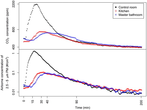
Figure 2 shows the airborne concentration of PM and CO₂ in the control room, kitchen and master bathroom as a function of time during Experiment M3. The dispersion of the injected fluorescent PM and CO₂ from the injection point in the control room to the kitchen and finally to the master bathroom (Figure 1) was evident in the time lag between the peak PM and CO₂ concentrations. For Experiment M3, approximately 90 min after the release of PM and CO₂, the concentrations in the three rooms approached the same value and followed the same decay curve, indicating that the PM and CO₂ were well mixed in the entire test house. A comparison of PM and CO₂ graphs in Figure 2 demonstrates that there is a high similarity between the concentration profiles of PM and CO₂. More precisely the figures show that the distribution of 3.2 µm particles – injected by releasing CO₂ at the same time and place as the PM – is the same as the distribution of CO₂. This indicates that even with the air conditioning fan off, the AV (caused by buoyancy forces and the airflow supplied by the DMV ventilation in the house) was sufficient to carry 3.2 µm particles in the same way as the tracer gas.

Figure 2. Concentrations of PM and CO₂ in the control room, kitchen and master bathroom during Experiment M3; the injection of particles and CO₂ occurred between time zero and 15 min.

The CO₂ concentration profiles measured during Experiments M2–M7 show that the DMV system had no impact on the dispersion of the tracer gas and corresponding particles between rooms. Specifically, statistical analysis indicates there was no significant difference between the air change rates (ACHs) measured in hidden spaces (Equation (1)(1) $$-\hspace{0.17em}\text{ln}\hspace{0.17em}\left[\frac{C(t)-C_{\mathit{room}}}{C(t=0)-C_{\mathit{room}}}\right]=\lambda t$$(1) ) when the DMV system was on versus when it was off (p = 0.80 for the master bedroom closet, and p = 0.09 for the kitchen drawer/cabinet space). However, the temperature field in the house did have a major impact. Depending on the temperature differences between rooms in the house, it took from 0.5 to 1.5 h until uniform concentration of CO₂ throughout the house was achieved. This time is often called the mixing time, which is the time required to achieve a uniform concentration in all rooms that is equivalent to the concertation that occurs with perfect mixing. For example, in Experiment M3 – which had the DMV system on and only a 0.4 °C temperature difference between the injection point in the control room and the adjacent kitchen – the mixing time was approximately 1.5 h. Conversely, in Experiments M5 which also had the DMV system on but a much higher temperature difference (1.0 °C) between these two rooms, the mixing time was approximately 0.5 h. In both of these experiments, the AHU was off, indicating that buoyancy-driven flow (reflected in the temperature difference between rooms) had a major impact on the distribution and movement of air throughout the house.

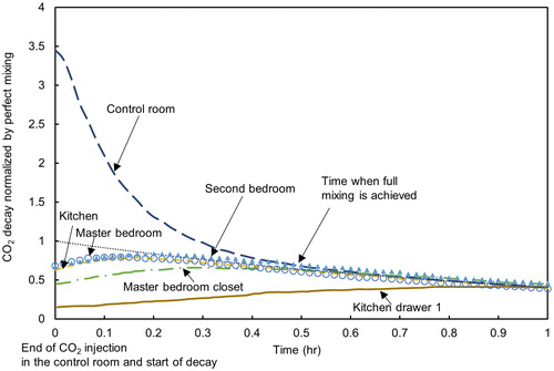
Figure 3 summarizes the dispersion of CO₂ and decay over time for Experiment M5 which is illustrative of the CO₂ profiles obtained in Experiments M2–M7. The y-axis shows the measured concentration of tracer gas normalized by the concentration of tracer gas that would happen throughout the whole house with perfect (instantaneous) mixing (values above 1 indicate concentrations greater than those with perfect mixing and vice versa). The graph in Figure 3 shows that the CO₂ concentration in the master bedroom closet quickly reached the concentration levels in the master bedroom and decayed at the same rate, indicating close communication between the closet and the master bedroom. In contrast, the CO₂ concentration in the kitchen drawer increased and decayed much slower with a greater time lag as compared to the CO₂ concentration in the kitchen. This indicates a lower communication rate between the kitchen drawer and the kitchen space in this experiment. Similar profiles were observed in the other injection experiments (M2–M7).

Figure 3. Temporal concentrations of CO₂ in the house and in the hidden spaces in Experiment M5 after injection of the tracer gas in the control room. Note: the CO₂ concentration measured during the decay test was normalized by the CO₂ concentration calculated for perfect mixing (unmarked dotted line) on the y-axis.

Overall, the results from experiments that measured CO₂ and PM dispersion indicate that rooms connected with open interior doors can be viewed as a single zone after a certain period of time. With the AHU system off, it took approximately 30–90 min to achieve perfect mixing and uniform dispersion of the 3.2 µm particles released from one corner of the house (control room in Figure 1). Furthermore, the results show that there was intensive airflow between closed closets and rooms while closed drawers interchanged air at a slower rate. However, regardless of the time lag, results of the CO₂ dispersion measurements indicate that there was sufficient air mixing between rooms as well as in-between hidden spaces and adjacent rooms to transport PM from the PM source position in the house to the indoor hidden spaces.

The current results are comparable to those reported in a previous study examining the transport of carbon monoxide (CO) emitted from smoking under similar experimental conditions (i.e., no heating or ventilation system, windows closed) (Ott, Klepeis, and Switzer 2003). When the door between the adjacent room and the source room where CO was released was opened a small crack (3 in), there was a substantial amount of CO detected in the adjacent room after smoking and the two rooms became well-mixed after about 50 min. Furthermore, a small amount of CO was found in a third room connected to the adjacent room by a closed door. The results are also consistent with those presented in the study by Bekö et al. (2016), which shows that the concentration of tracer gas is nearly uniform on the same floor as the source room. Another study by Ferro et al. (2009) found that a small door opening (2.5 cm width) could introduce significantly more tracer gas to a receptor room from the source room compared with a fully closed or sealed door. However, even in the case of a closed door, the concentration of tracer gas in the receptor room could reach as high as 43% (4-h average) of the concentration in the source room. The impact of door gaps on tracer gas concentration as reported by Ferro et al. (2009) are consistent with the findings in the current study in that the gap below the closed closet doors allowed air to circulate intensely. In contrast, the closed drawers in the current study were more air-tight and prevented the tracer gas from entering effectively. However, some penetration of the tracer gas and PM occurred indicating that there were tiny gaps around the closed drawers.

Deposition of fluorescent aerosols

Figure 4 shows the normalized surface concentrations of fluorescent PM for all seven aerosol injection experiments. The surface concentrations measured at each sampling location were normalized by the surface concentration measured in the kitchen area for each of the seven experiments. In this way, it is possible to directly compare the results of one experiment to another even though the number of particles injected in the control room in a given experiment varied somewhat due to the aerosol injection methodology deployed in this study. The kitchen was selected as the normalization point since it is the central space for the whole house and connected to almost all of the surface measurement points. As a result of the normalization process, all normalized concentration results for the kitchen shown in Figure 4 have a value of 1.

Figure 4. Normalized surface concentrations of fluorescent PM on the sampling slides in Experiments M1–M7. Experiments M5 and M6 are duplicate experiments with dedicated mechanical ventilation (DMV) on, while Experiments M4 and M7 are duplicate experiments with DMV off. Note that samples were collected from the two kitchen drawers for all experiments except M1–M3. The symbols represent the averages of PM on the three or five sampling slides at the same location, and the error bars represent SDs. Locations: CR – control room, SR – second bedroom, KR – kitchen, MR – master bedroom, MB – master bathroom, SRC – second bedroom closet, MRC – master bedroom closet, MBC – master bathroom cabinet, KRD 1 – kitchen drawer 1, KRD 2 – kitchen drawer 2.

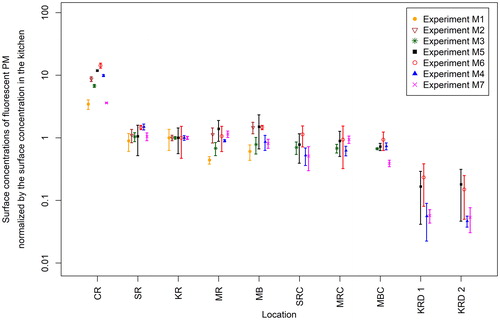
The normalized surface concentration profiles across the house summarized in Figure 4 indicate that the concentration of PM deposited onto the floor of the source room (i.e., the control room) was approximately 3–14 times greater than that deposited onto the floor of the kitchen. In addition to the observation of similar surface concentrations of PM on the floor of all the rooms (except for the source room), similar levels of PM were found on: (1) the upper surface of the shelf in the closed closet in the second bedroom (SRC) (a ratio of 0.35–0.77 to the PM level in the second bedroom [SR]), (2) the floor in the closed closet in the master bedroom (MRC) (a ratio of 0.64–1 to the PM level in the master bedroom [MR]), and (3) the bottom of the open-door cabinet in the master bathroom (MBC) (a ratio of 0.48–0.86 to the PM level in the master bathroom [MB]). Furthermore, there were fewer but detectable levels of fluorescent particles in the two closed kitchen drawers (KRD 1 and KRD 2) with a ratio of 0.05–0.23 of the PM level in the kitchen (KR).

With respect to the effect of operating the DMV system (on or off conditions in various experiments), the results in Figure 4 indicate that there was no significant difference in the PM deposition as a function of DMV system operation. These results clearly indicate that even without mechanically driven flow (AHU and/or DMV), aerosols injected into the interior space can mix well throughout the space over time. This led to a relatively even deposition of the PM on the floor of the rooms and even within the closets which had their doors closed. Of particular note is the finding that the injected particles readily penetrated into hidden spaces such as closed drawers within closed cabinets where the exchange of gases and PM between the room and the hidden space was expected to be much smaller. Similar results were reported by Miller and Nazaroff (2001) who found that the number concentration of environmental tobacco smoke particles in the nonsmoking room approached the concentration in the smoking room shortly after cigarette ignition if the door connecting the two rooms was open, and was much smaller in the nonsmoking room if the door was closed.

For each aerosol injection experiment (M1–M7), the temperature measured in each room and hidden space were averaged over a 6-h period after the injection of fluorescent particles. The time-averaged temperature data were subsequently normalized by subtracting the time-averaged room temperature in the kitchen for each experiment (Figure 5).

Figure 5. Normalized time-averaged temperature in rooms, the master bedroom closet and kitchen drawer 1 in Experiments M1–M7. Locations: CR – control room, SR – second bedroom, KR – kitchen, MR – master bedroom, MB – master bathroom, MRC – master bedroom closet, KRD 1 – kitchen drawer 1.

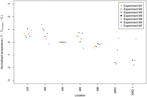
As noted earlier (in the discussion of mixing time for tracer gas and aerosols), the greater the temperature difference observed between the control room and the other rooms in the house, the shorter the measured mixing time required to distribute the gas and PM tracers throughout the main rooms in the house. With respect to the hidden spaces, the measured air temperature differences between the master bedroom closet and the master bedroom were 0.8–2.0 °C, and the measured air temperature differences between the kitchen drawer 1 and the kitchen were 0.3–1.8 °C. The outdoor weather conditions varied in different experiments, and it indirectly affected the temperature difference between occupied and hidden spaces. In Experiments M4–M6, the temperatures in the hidden space (drawer or closet) were cooler than the adjacent room; these temperature differences reflect that these three experiments were conducted in August and September when the house was cooled with the HVAC system on prior to initiating the experiments. In contrast, Experiment M7 was conducted on a cold day in February and the temperatures inside the closets and drawers in Experiment M7 were warmer than the adjacent room temperature. It is hypothesized that the temperature differences measured between rooms and between hidden spaces and adjacent rooms may contribute to air mixing that distributed PM and gases throughout the house and even into hidden spaces.

Air velocities and ACHs in closets and drawers

To quantify the airflow rates between the room spaces and hidden spaces, the air change rates per hour (ACHs) between the master bedroom closet and the master bedroom, and one kitchen drawer and the kitchen were measured (Experiments HAC 1–HAC 6 in Table 1). Results from these experiments are summarized in Figure 6. The average ACH measured in the master bedroom closet was 2.3 h⁻¹ which is reasonably consistent with the 4.3 h⁻¹ ACH measured previously for the same master bedroom closet (Guerrero and Corsi 2012), especially given the large range of ACH values measured in the current study. In contrast, the average ACH of the kitchen drawer/cabinet space was 1.5 h⁻¹ which was expected given the lower communication between these spaces.

Figure 6. ACHs in the master bedroom closet and the kitchen drawer/cabinet space as a function of the air temperature difference between the master bedroom closet and the master bedroom, and the kitchen drawer/cabinet space and the kitchen. The symbols represent the averages of three measurements in the master bedroom closet or the kitchen drawer/cabinet space, and the error bars represent SDs.

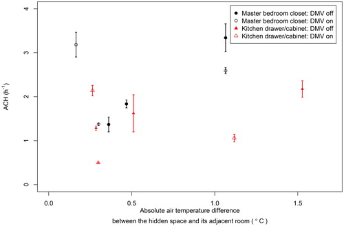
The measured ACHs of hidden spaces under the two operating conditions (On or Off) of the DMV system were not significantly different (master bedroom closet: p = 0.80, kitchen drawer/cabinet space: p = 0.09), a result which is consistent with the similar AV measured when the HVAC system was on and when it was off (see Table 3). However, no correlation was found between the ACHs measured in the hidden spaces and the magnitudes of the temperature differences between the hidden spaces and the corresponding adjacent rooms (master bedroom closet: Spearman correlation coefficient = 0.28, p = 0.27; kitchen drawer/cabinet: Spearman correlation coefficient = 0.02, p = 0.93). One possible explanation for the high ACH measured in the master bedroom closet (3.18 h⁻¹) at a small temperature difference (0.16 °C) is that the measured air temperature in the closet and adjacent space does not fully represent the buoyancy forces that drove air circulation measured in the hidden spaces. It is possible that surface–air temperature differences in the closet cabinets and drawers (which were not measured) may be more relevant for the buoyancy-driven flow in these hidden spaces.

Table 3. Air velocities (average ± SD, m/s) in the closet, cabinet and drawer.

Location	Kitchen drawer 1	Master bedroom closet shelf	Master bedroom closet floor	Master bathroom cabinet
AHU’s fan on	0.0515 ± 0.0017	0.0478 ± 0.0027	0.0517 ± 0.0042	0.0478 ± 0.0027
AHU’s fan off	0.0500 ± 0.0014	0.0480 ± 0.0012	0.0495 ± 0.0019	0.0480 ± 0.0016

To investigate the possibility that momentum-driven flow in the main space (room) drove the air circulation in hidden spaces, two additional AV experiments (Experiments AV 1 and AV 2 in Table 1) were completed to compare the AV in the hidden spaces when the central AHU was on and when the central AHU was off. Table 3 summarizes these results.

When the AHU’s fan was on, the average room AV was 0.1 m/s (equivalent to 8 ACHs in the house) and the velocity field in the rooms was dominated by the air circulation driven by the fan. When the AHU’s fan was off, the average rooms AV was significantly smaller: 0.05 m/s. Regardless, the velocities measured in the hidden spaces with the AHU’s fan on or off show there was little impact of the momentum-driven flow (air circulation in the house) on the airflow to these hidden spaces. Thus, the operation of the air conditioning system did not change the AV inside the hidden spaces. These results further imply that the momentum in the airflow resulting from the air conditioning fan systems or mechanical ventilation dissipated before the airflow entered the hidden spaces. Thus, considering the absence of a clear correlation between ACH and the air temperature difference between hidden spaces and their adjacent rooms in Figure 6, it is most likely that the temperature difference between the surfaces in the hidden space and air in the hidden space was driving this airflow.

Implications and limitations of the study results

Previous studies have examined hidden spaces (e.g., crawl spaces [Airaksinen, Pasanen, et al. 2004] and wall cavities [Muise and Seo 2009]) primarily as a source of contamination, with fewer studies examining how airborne PM penetrates into hidden interior spaces. The practical finding of the current study is that regardless of whether the ventilation and air conditioning system is operating, a measurable fraction of airborne particles (potentially contaminated with pathogens, heavy metals, SVOCs or other pollutants) can reach indoor hidden spaces distant from the source. Such information is critical for identifying the active surfaces for processes driven by surface chemistry or microbial activities in studies on indoor chemistry. For example, the results are crucial to a campaign focusing on the transport of chemicals via air and through partitioning between the gas phase and indoor PM conducted in the same UTest house (Farmer et al. 2019). Another implication of this study is about the occupant exposure risk to indoor aerosols. Most cleaning interventions to reduce indoor occupant exposures to chemical and biological pollutants associated with PM focus on vacuuming, wet mopping or surface cleaning of areas (e.g., flooring, windowsills, bedding or furniture surfaces) visible to view (Adgate et al. 2008; Ettinger et al. 2002; Kolarik, Bornehag, et al. 2008; Kwan et al. 2018; McConnell et al. 2003; Skulberg et al. 2004; Vojta et al. 2001). While there is recognition that hidden reservoirs are also of concern, particularly for fungi that grow on water-damaged materials found in wall cavities and other nonvisible areas (Anton, Moularat, and Robine 2016; Johansson, Svensson, and Ekstrand-Tobin 2013), the result of the current study highlights the fact that PM-associated contaminants can penetrate into closed closets and drawers and thus accumulate on surfaces that are in direct contact with occupants (i.e., dishes, clothing or other materials stored in drawers, cabinets, and closets). Such phenomena may be of particular concern in sensitive environments such as hospitals where the roles of ward cleanliness and environmental transmission of pathogens in hospital-acquired infections continue to be an active area of research (Beggs et al. 2015). Similarly, the results of the current study suggest that using a closet (even with a closed door) as a shelter-in-place strategy (Sorensen 2002) from indoor aerosols may not be effective unless the gap under the door is blocked. Finally, this study can also help explain the cause of the transport of air pollutants out of hidden spaces if there are emission sources inside these confined spaces, that is, buoyancy-driven flow is sufficient to move gas and PM out of hidden spaces.

The current study provides insight into the fraction of aerosols released indoors that penetrate into specific types of hidden interior spaces, specifically drawers, cabinets and closets. However, as the study results are based on a specific building (a full-scale house) and just one size of particles, the values reported in Figure 4 cannot be directly translated to all homes and all particle sizes. Nevertheless, the relative magnitude of aerosol transport from a source room to distant interior cavities (such as cabinets and drawers) measured in this study can serve as a reference for other studies that focus on the fate of indoor airborne particles in other buildings. With respect to residential homes, similar trends are expected in most homes where the doors between rooms are kept open. The study also identifies construction factors that appear to affect PM transport. Specifically, the results indicate that the size of the opening that connects the hidden and occupied space affects PM transport with, for example, substantially greater transport of PM through a closed but undercut door relative to that through the tiny gaps in cabinets and drawers. We would expect that these findings will extend to other homes, but we also acknowledge that there are additional possibilities for PM transport driven by specifics of the construction and building type. For instance, cracks in walls and pressure differences between spaces (a phenomenon not examined in this study) can drive air and PM movement to these spaces (Liu and Nazaroff 2003). Additionally, the HVAC fan was kept off in the aerosol and tracer gas experiments in this study, but the operation of the HVAC fan would change the dispersion of tracer gas and possibly PM throughout the house. Due to the mixing effect of the HVAC system, tracer gas and aerosols will be well mixed in open rooms at a faster rate when the HVAC is on as compared to the situation when it is off. However, as the momentum-driven flow provided by the HVAC system proves not to be the reason for the transport of aerosols into hidden spaces (Table 3), it is still buoyancy-driven flow that will move PM into hidden spaces regardless of the operating conditions of the HVAC system. Therefore, the results of PM deposition in hidden spaces can be generalized to the conditions when the HVAC system is on.

Conclusions

This article presents the results from a full-scale investigation that tracked the movement of air (using a tracer gas) and indoor aerosols (using fluorescent particles) to determine the dispersion of aerosols throughout a house and ultimately into hidden spaces within the interior of the house. Intensive air circulation between rooms and adjacent closed closets and cabinets was found, and the aerosols deposited within the closets and cabinet were comparable to those in the rooms. As for more sealed spaces like the closed drawers within closed cabinets, the increase of tracer gas and deposition of aerosols was small but detectable. These results indicate that aerosols and gases can readily penetrate hidden spaces. The magnitude of aerosol deposition between the source area and the most hidden space in the house (e.g., drawer) declined by two orders of magnitude. Nonetheless, the results indicate that at least one percent of an indoor aerosol source can deposit into indoor hidden spaces and accumulate.

The current study indicates that even when the fan of the air conditioning system and the DMV system were off, air circulation due to temperature differences between the rooms was sufficient to disperse the aerosol throughout all areas of the building. The injected aerosols and tracer gas eventually became well mixed throughout the rooms, and the injected PM deposited onto the floors in a relatively uniform manner. Indoor hidden spaces such as closets and drawers that are not directly visible were found to be well connected to the occupied space. Even for closed closet doors, for instance, gaps beneath the door may facilitate the flow of air in and out. Momentum driven flow (such as air circulation driven by an air-conditioning fan) had negligible effect on air circulation in hidden spaces as the momentum dissipated before entering the hidden spaces. Therefore, the results suggest that the penetration of aerosols into hidden places is dominated by buoyancy flow induced by temperature differences. Additional studies on the impact of buoyancy on air circulation in hidden spaces would be useful to further characterize this effect.

Acknowledgment

The access to the fluorescence stereoscope used in this research was provided by the Microscopy and Imaging Facility of the Center for Biomedical Research Support at The University of Texas at Austin.

Additional information

Funding

The authors would like to thank the Alfred P. Sloan Foundation for funding the Hidden Spaces Project (Grant No. G-2016-7203).

References

- Adams, R. I., D. S. Lymperopoulou, P. K. Misztal, R. De Cassia Pessotti, S. W. Behie, Y. Tian, A. H. Goldstein, S. E. Lindow, W. W. Nazaroff, J. W. Taylor, et al. 2017. Microbes and associated soluble and volatile chemicals on periodically wet household surfaces. Microbiome 5 (1):128. doi:10.1186/s40168-017-0347-6.
- Adgate, J. L., G. Ramachandran, S. J. Cho, A. D. Ryan, and J. Grengs. 2008. Allergen levels in inner city homes: Baseline concentrations and evaluation of intervention effectiveness. J. Exp. Sci. Environ. Epidemiol. 18 (4):430–440. doi:10.1038/sj.jes.7500638.
- Airaksinen, M., J. Kurnitski, P. Pasanen, and O. Seppänen. 2004. Fungal spore transport through a building structure. Indoor Air 14 (2):92–104. doi:10.1046/j.1600-0668.2003.00215.x.
- Airaksinen, M., P. Pasanen, J. Kurnitski, and O. Seppänen. 2004. Microbial contamination of indoor air due to leakages from crawl space: A field study. Indoor Air 14 (1):55–64. doi:10.1046/j.1600-0668.2003.00210.x.
- Anton, R., S. Moularat, and E. Robine. 2016. A new approach to detect early or hidden fungal development in indoor environments. Chemosphere 143:41–49. doi:10.1016/j.chemosphere.2015.06.072.
- Barberan, A., R. R. Dunn, B. J. Reich, K. Pacifici, E. B. Laber, H. L. Menninger, J. M. Morton, J. B. Henley, J. W. Leff, S. L. Miller, et al. 2015. The ecology of microscopic life in household dust. Proc. Roy. Soc. B: Biol. Sci. 282:20151139. doi:10.1098/rspb.2015.1139.
- Beggs, C., L. D. Knibbs, G. R. Johnson, and L. Morawska. 2015. Environmental contamination and hospital-acquired infection: Factors that are easily overlooked. Indoor Air 25 (5):462–474. doi:10.1111/ina.12170.
- Bekö, G., S. Gustavsen, M. Frederiksen, N. C. Bergsøe, B. Kolarik, L. Gunnarsen, J. Toftum, and G. Clausen. 2016. Diurnal and seasonal variation in air exchange rates and interzonal airflows measured by active and passive tracer gas in homes. Build. Environ. 104:178–187. doi:10.1016/j.buildenv.2016.05.016.
- Bok, G., N. Hallenberg, and O. Åberg. 2009. Mass occurrence of penicillium corylophilum in crawl spaces, South sweden. Build. Environ. 44 (12):2413–2417. doi:10.1016/j.buildenv.2009.04.001.
- Boor, B. E., J. A. Siegel, and A. Novoselac. 2013a. Monolayer and multilayer particle deposits on hard surfaces: Literature review and implications for particle resuspension in the indoor environment. Aeros. Sci. Technol. 47 (8):831–847. doi:10.1080/02786826.2013.794928.
- Boor, B. E., J. A. Siegel, and A. Novoselac. 2013b. Wind tunnel study on aerodynamic particle resuspension from monolayer and multilayer deposits on linoleum flooring and galvanized sheet metal. Aeros. Sci. Technol. 47 (8):848–857. doi:10.1080/02786826.2013.794929.
- Boor, B. E., M. P. Spilak, R. L. Corsi, and A. Novoselac. 2015. Characterizing particle resuspension from mattresses: Chamber study. Indoor Air 25 (4):441–456. doi:10.1111/ina.12148.
- Cetin, K. S., and A. Novoselac. 2015. Single and multi-family residential central all-air HVAC system operational characteristics in cooling-dominated climate. Energy Build. 96:210–220. doi:10.1016/j.enbuild.2015.03.039.
- Chang, J. C. S., and K. A. Krebs. 1992. Evaluation of para-dichlorobenzene emissions from solid moth repellant as a source of indoor air pollution. J. Air Waste Manage. Assoc. 42 (9):1214–1217. doi:10.1080/10473289.1992.10467071.
- Dodson, R. E., L. J. Perovich, A. Covaci, N. Van Den Eede, A. C. Ionas, A. C. Dirtu, J. G. Brody, and R. A. Rudel. 2012. After the PBDE phase-out: A broad suite of flame retardants in repeat house dust samples from California. Environ. Sci. Technol. 46 (24):13056–13066. doi:10.1021/es303879n.
- Doekes, G., B. Brunekreef, J. Douwes, F. van Leusden, R. van Strien, L. Wijnands, B. van der Sluis, and A. Verhoeff. 2005. Fungal extracellular polysaccharides in house dust as a marker for exposure to fungi: Relations with culturable fungi, reported home dampness, and respiratory symptoms. J. Allergy Clin. Immunol. 103:494–500. doi:10.1016/S0091-6749(99)70476-8.
- Douwes, J., P. Thorne, N. Pearce, and D. Heederik. 2003. Bioaerosol health effects and exposure assessment: Progress and prospects. Ann. Occup. Hyg. 47:187–200. doi:10.1093/annhyg/meg032.
- El Orch, Z., B. Stephens, and M. S. Waring. 2014. Predictions and determinants of size-resolved particle infiltration factors in single-family homes in the U.S. Build. Environ. 74:106–118. doi:10.1016/j.buildenv.2014.01.006.
- Estrada-Perez, C. E., J. P. Maestre, K. A. Kinney, M. D. King, and Y. A. Hassan. 2018. Droplet distribution and airborne bacteria in an experimental shower unit. Water Res. 130:47–57. doi:10.1016/j.watres.2017.11.039.
- Ettinger, A. S., R. L. Bornschein, M. Farfel, C. Campbell, N. B. Ragan, G. G. Rhoads, M. Brophy, S. Wilkens, and D. W. Dockery. 2002. Assessment of cleaning to control lead dust in homes of children with moderate lead poisoning: Treatment of lead-exposed children trial. Environ. Health Perspect. 110 (12):A773–A779. doi:10.1289/ehp.021100773.
- Farmer, D. K., M. E. Vance, J. P. D. Abbatt, A. Abeleira, M. R. Alves, C. Arata, E. Boedicker, S. Bourne, F. Cardoso-Saldaña, R. Corsi, et al. 2019. Overview of HOMEChem: House observations of microbial and environmental chemistry. Environ. Sci. Proc. Impacts 21:1280–1300. doi:10.1039/C9EM00228F.
- Ferro, A. R., N. E. Klepeis, W. R. Ott, W. W. Nazaroff, L. M. Hildemann, and P. Switzer. 2009. Effect of interior door position on room-to-room differences in residential pollutant concentrations after short-term releases. Atmos. Environ. 43 (3):706–714. doi:10.1016/j.atmosenv.2008.09.032.
- Ferro, A. R., R. J. Kopperud, and L. M. Hildemann. 2004. Source strengths for indoor human activities that resuspend particulate matter. Environ. Sci. Technol. 38 (6):1759–1764. doi:10.1021/es0263893.
- Glorennec, P., J.-P. Lucas, C. Mandin, and B. L. Bot. 2012. French children’s exposure to metals via ingestion of indoor dust, outdoor playground dust and soil: Contamination data. Environ. Int. 45:129–134. doi:10.1016/j.envint.2012.04.010.
- Guerrero, P. A., and R. L. Corsi. 2012. Emissions of p-dichlorobenzene and naphthalene from consumer products. J. Air Waste Manage. Assoc. 62 (9):1075–1084. doi:10.1080/10962247.2012.694399.
- Happo, M., A. Markkanen, P. Markkanen, P. Jalava, K. Kuuspalo, A. Leskinen, O. Sippula, K. Lehtinen, J. Jokiniemi, and M. R. Hirvonen. 2013. Seasonal variation in the toxicological properties of size-segregated indoor and outdoor air particulate matter. Toxicol. In Vitro 27 (5):1550–1561. doi:10.1016/j.tiv.2013.04.001.
- Hayashi, M., H. Osawa, K. Hasegawa, and Y. Honma. 2014. Numerical experiments on indoor air quality considering infiltration of mould from crawl space. J. Environ. Protect. 5 (10):835–844. doi:10.4236/jep.2014.510086.
- Hoek, G., G. Kos, R. Harrison, J. de Hartog, K. Meliefste, H. ten Brink, K. Katsouyanni, A. Karakatsani, M. Lianou, A. Kotronarou, et al. 2008. Indoor-outdoor relationships of particle number and mass in four European cities. Atmos. Environ. 42 (1):156–169. doi:10.1016/j.atmosenv.2007.09.026.
- Hospodsky, D., J. Qian, W. W. Nazaroff, N. Yamamoto, K. Bibby, H. Rismani-Yazdi, and J. Peccia. 2012. Human occupancy as a source of indoor airborne bacteria. PLoS One 7 (4):e34867. doi:10.1371/journal.pone.0034867.
- Hospodsky, D., N. Yamamoto, W. W. Nazaroff, D. Miller, S. Gorthala, and J. Peccia. 2015. Characterizing airborne fungal and bacterial concentrations and emission rates in six occupied children’s classrooms. Indoor Air 25 (6):641–652. doi:10.1111/ina.12172.
- Hussein, T., T. Glytsos, J. Ondráček, P. Dohányosová, V. Ždímal, K. Hämeri, M. Lazaridis, J. Smolík, and M. Kulmala. 2006. Particle size characterization and emission rates during indoor activities in a house. Atmos. Environ. 40 (23):4285–4307. doi:10.1016/j.atmosenv.2006.03.053.
- Johansson, P., T. Svensson, and A. Ekstrand-Tobin. 2013. Validation of critical moisture conditions for mould growth on building materials. Build. Environ. 62:201–209. doi:10.1016/j.buildenv.2013.01.012.
- Ju, C., and J. D. Spengler. 1981. Room-to-room variations in concentration of respirable particles in residences. Environ. Sci. Technol. 15 (5):592–596. doi:10.1021/es00087a600.
- Keskikuru, T., J. Salo, P. Huttunen, H. Kokotti, M. Hyttinen, R. Halonen, and J. Vinha. 2018. Radon, fungal spores and MVOCs reduction in crawl space house: A case study and crawl space development by hygrothermal modelling. Build. Environ. 138:1–10. doi:10.1016/j.buildenv.2018.04.026.
- Kolarik, B., C.-G. Bornehag, K. Naydenov, J. Sundell, P. Stavova, and O. F. Nielsen. 2008. The concentrations of phthalates in settled dust in Bulgarian homes in relation to building characteristic and cleaning habits in the family. Atmos. Environ. 42 (37):8553–8559. doi:10.1016/j.atmosenv.2008.08.028.
- Kolarik, B., K. Naydenov, M. Larsson, C.-G. Bornehag, and J. Sundell. 2008. The association between phthalates in dust and allergic diseases among bulgarian children. Environ. Health Perspect. 116 (1):98–103. doi:10.1289/ehp.10498.
- Krauter, P., A. Biermann, and L. D. Larsen. 2005. Transport efficiency and deposition velocity of fluidized spores in ventilation ducts. Aerobiologia 21 (3–4):155–172. doi:10.1007/s10453-005-9001-z.
- Kwan, S. E., R. J. Shaughnessy, B. Hegarty, U. Haverinen-Shaughnessy, and J. Peccia. 2018. The reestablishment of microbial communities after surface cleaning in schools. J. Appl. Microbiol. 125 (3):897–906. doi:10.1111/jam.13898.
- Langer, S., M. Fredricsson, C. J. Weschler, G. Bekö, B. Strandberg, M. Remberger, J. Toftum, and G. Clausen. 2016. Organophosphate esters in dust samples collected from Danish homes and daycare centers. Chemosphere 154:559–566. doi:10.1016/j.chemosphere.2016.04.016.
- Liu, D.-L., and W. W. Nazaroff. 2003. Particle penetration through building cracks. Aerosol Sci. Technol. 37 (7):565–573. doi:10.1080/02786820300927.
- Long, C. M., H. H. Suh, L. Kobzik, P. J. Catalano, Y. Y. Ning, and P. Koutrakis. 2001. A pilot investigation of the relative toxicity of indoor and outdoor fine particles: In vitro effects of endotoxin and other particulate properties. Environ. Health Perspect. 109 (10):1019–1026. doi:10.1289/ehp.011091019.
- Long, C. M., H. H. Suh, and P. Koutrakis. 2000. Characterization of indoor particle sources using continuous mass and size monitors. J. Air Waste Manage. Assoc. 50 (7):1236–1250. doi:10.1080/10473289.2000.10464154.
- McConnell, R., C. Jones, J. Milam, P. Gonzalez, K. Berhane, L. Clement, J. Richardson, J. Hanley-Lopez, K. Kwong, N. Maalouf, et al. 2003. Cockroach counts and house dust allergen concentrations after professional cockroach control and cleaning. Ann. Allergy Asthma Immunol. 91 (6):546–552. doi:10.1016/S1081-1206(10)61532-3.
- Miller, S. L., and W. W. Nazaroff. 2001. Environmental tobacco smoke particles in multizone indoor environments. Atmos. Environ. 35 (12):2053–2067. doi:10.1016/S1352-2310(00)00506-9.
- Monn, C., and S. Becker. 1999. Cytotoxicity and induction of proinflammatory cytokines from human monocytes exposed to fine (PM2.5) and coarse particles (PM10-2.5) in outdoor and indoor air. Toxicol. Appl. Pharmacol. 155 (3):245–252. doi:10.1006/taap.1998.8591.
- Muise, B., and D.-C. Seo. 2009. Lateral fungal spore movement inside a simulated wall. Aerobiologia. 25 (1):7–14. doi:10.1007/s10453-008-9103-5.
- Naumova, Y. Y., S. J. Eisenreich, B. J. Turpin, C. P. Weisel, M. T. Morandi, S. D. Colome, L. A. Totten, T. H. Stock, A. M. Winer, S. Alimokhtari, et al. 2002. Polycyclic aromatic hydrocarbons in the indoor and outdoor air of three cities in the U.S. Environ. Sci. Technol. 36 (12):2552–2559. doi:10.1021/es015727h.
- Nazaroff, W. W. 2004. Indoor particle dynamics. Indoor Air 14 (s7):175–183. doi:10.1111/j.1600-0668.2004.00286.x.
- Ogulei, D., P. K. Hopke, and L. A. Wallace. 2006. Analysis of indoor particle size distributions in an occupied townhouse using positive matrix factorization. Indoor Air 16 (3):204–215. doi:10.1111/j.1600-0668.2006.00418.x.
- Ormstad, H. 2000. Suspended particulate matter in indoor air: Adjuvants and allergen carriers. Toxicology 152 (1–3):53–68. doi:10.1016/S0300-483X(00)00292-4.
- Ott, W. R., N. E. Klepeis, and P. Switzer. 2003. Analytical solutions to compartmental indoor air quality models with application to environmental tobacco smoke concentrations measured in a house. J. Air Waste Manage. Assoc. 53 (8):918–936. doi:10.1080/10473289.2003.10466248.
- Pessi, A.-M., J. Suonketo, M. Pentti, M. Kurkilahti, K. Peltola, and A. Rantio-Lehtimaki. 2002. Microbial growth inside insulated external walls as an indoor air biocontamination source. Appl. Environ. Microbiol. 68 (2):963–967. doi:10.1128/AEM.68.2.963-967.2002.
- Prussin, A. J., and L. C. Marr. 2015. Sources of airborne microorganisms in the built environment. Microbiome 3 (1):78–78. doi:10.1186/s40168-015-0144-z.
- Qian, J., D. Hospodsky, N. Yamamoto, W. W. Nazaroff, and J. Peccia. 2012. Size-resolved emission rates of airborne bacteria and fungi in an occupied classroom. Indoor Air 22 (4):339–351. doi:10.1111/j.1600-0668.2012.00769.x.
- Rao, J., G. Miao, D. Q. Yang, K. Bartlett, and P. Fazio. 2006. Experimental evaluation of potential movement of airborne mold spores out of building envelope cavities using full size wall panels. In Research in building physics and building engineering, ed. P. Fazio, J. Rao, and G. Desmarais, 845–852. London: Taylor & Francis.
- Rasmussen, P. E., C. Levesque, M. Chénier, and H. D. Gardner. 2018. Contribution of metals in resuspended dust to indoor and personal inhalation exposures: Relationships between PM10 and settled dust. Build. Environ. 143:513–522. doi:10.1016/j.buildenv.2018.07.044.
- Rim, D., and A. Novoselac. 2008. Transient simulation of airflow and pollutant dispersion under mixing flow and buoyancy driven flow regimes in residential buildings. ASHRAE Trans. 114:130–142.
- Satsangi, P. G., S. Yadav, A. S. Pipal, and N. Kumbhar. 2014. Characteristics of trace metals in fine (PM2.5) and inhalable (PM10) particles and its health risk assessment along with in-silico approach in indoor environment of India. Atmos. Environ. 92:384–393. doi:10.1016/j.atmosenv.2014.04.047.
- Shao, L., J. Li, H. Zhao, S. Yang, H. Li, W. Li, T. Jones, K. Sexton, and K. BéruBé. 2007. Associations between particle physicochemical characteristics and oxidative capacity: An indoor PM10 study in Beijing, China. Atmos. Environ. 41 (26):5316–5326. doi:10.1016/j.atmosenv.2007.02.038.
- Siegel, J. A., and I. S. Walker. 2001. Deposition of biological aerosols on HVAC heat exchangers. Berkeley, CA: Lawrence Berkeley National Laboratory (LBNL).
- Skulberg, K. R., K. Skyberg, K. Kruse, W. Eduard, P. Djupesland, F. Levy, and H. Kjuus. 2004. The effect of cleaning on dust and the health of office workers: An intervention study. Epidemiology 15 (1):71–78. doi:10.1097/01.ede.0000101020.72399.37.
- Sorensen, J. H. 2002. Will duct tape and plastic really work? Issues related to expedient shelter-in-place. Accessed September 29, 2019. https://www.osti.gov/servlets/purl/814573.
- Spilak, M. P., B. E. Boor, A. Novoselac, and R. L. Corsi. 2014. Impact of bedding arrangements, pillows, and blankets on particle resuspension in the sleep microenvironment. Build. Environ. 81:60–68. doi:10.1016/j.buildenv.2014.06.010.
- Srikanth, P., S. Sudharsanam, and R. Steinberg. 2008. Bio-aerosols in indoor environment: Composition, health effects and analysis. Indian J. Med. Microbiol. 26 (4):302–312. doi:10.4103/0255-0857.43555.
- Stapleton, H. M., S. Klosterhaus, S. Eagle, J. Fuh, J. D. Meeker, A. Blum, and T. F. Webster. 2009. Detection of organophosphate flame retardants in furniture foam and U.S. House dust. Environ. Sci. Technol. 43 (19):7490–7495. doi:10.1021/es9014019.
- Täubel, M., H. Rintala, M. Pitkäranta, L. Paulin, S. Laitinen, J. Pekkanen, A. Hyvärinen, and A. Nevalainen. 2009. The occupant as a source of house dust bacteria. J. Allergy Clin. Immunol. 124 (4):834. doi:10.1016/j.jaci.2009.07.045.
- Thatcher, T. L., A. C. K. Lai, R. Moreno-Jackson, R. G. Sextro, and W. W. Nazaroff. 2002. Effects of room furnishings and air speed on particle deposition rates indoors. Atmos. Environ. 36 (11):1811–1819. doi:10.1016/S1352-2310(02)00157-7.
- Touchie, M. F., and J. A. Siegel. 2018. Residential HVAC runtime from smart thermostats: Characterization, comparison, and impacts. Indoor Air 28 (6):905–915. doi:10.1111/ina.12496.
- Turner, A., and L. Simmonds. 2006. Elemental concentrations and metal bioaccessibility in UK household dust. Sci. Total Environ. 371 (1–3):74–81. doi:10.1016/j.scitotenv.2006.08.011.
- Vojta, P. J., S. P. Randels, J. Stout, M. Muilenberg, H. A. Burge, H. Lynn, H. Mitchell, G. T. O’Connor, and D. C. Zeldin. 2001. Effects of physical interventions on house dust mite allergen levels in carpet, bed and upholstery dust in low-income, urban homes. Environ. Health Perspect. 109 (8):815–819. doi:10.1289/ehp.01109815.
- Wainman, T., J. Zhang, C. J. Weschler, and P. J. Lioy. 2000. Ozone and limonene in indoor air: A source of submicron particle exposure. Environ. Health Perspect. 108 (12):1139–1145. doi:10.1289/ehp.001081139.
- Wallace, L. 1996. Indoor particles: A review. J. Air Waste Manage. Assoc. 46 (2):98–126. doi:10.1080/10473289.1996.10467451.
- Wang, F., Y. Zhou, D. Meng, M. Han, and C. Jia. 2018. Heavy metal characteristics and health risk assessment of PM2.5 in three residential homes during winter in Nanjing, China. Build. Environ. 143:339–348. doi:10.1016/j.buildenv.2018.07.011.
- Waring, M. S., and J. A. Siegel. 2008. Particle loading rates for HVAC filters, heat exchangers, and ducts. Indoor Air 18 (3):209–224. doi:10.1111/j.1600-0668.2008.00518.x.
- Weikl, F., C. Tischer, A. J. Probst, J. Heinrich, I. Markevych, S. Jochner, and K. Pritsch. 2016. Fungal and bacterial communities in indoor dust follow different environmental determinants. PLoS One 11 (4):e0154131–15. doi:10.1371/journal.pone.0154131.
- Wilford, B. H., M. Shoeib, T. Harner, J. Zhu, and K. C. Jones. 2005. Polybrominated diphenyl ethers in indoor dust in Ottawa, Canada: Implications for sources and exposure. Environ. Sci. Technol. 39 (18):7027–7035. doi:10.1021/es050759g.
- Wu, Y., A. Chen, I. Luhung, E. T. Gall, Q. Cao, V. W. C. Chang, and W. W. Nazaroff. 2016. Bioaerosol deposition on an air-conditioning cooling coil. Atmos. Environ. 144:257–265. doi:10.1016/j.atmosenv.2016.09.004.
- Zhou, B., B. Zhao, and Z. Tan. 2011. How particle resuspension from inner surfaces of ventilation ducts affects indoor air quality—A modeling analysis. Aeros. Sci. Technol. 45 (8):996–1009. doi:10.1080/02786826.2011.576281.