New approaches to calculate the transfer function of particle mass analyzers

Abstract

This article provides an overview of methods to evaluate transfer functions for the Couette centrifugal particle mass analyzer (CPMA) and aerosol particle mass analyzer (APM). The work first considers finite difference approaches to solving the partial differential equation governing particle motion, which represents an accurate but computationally-demanding approach to evaluating the transfer function. This is used as a baseline to compare to particle tracking methods, which have been shown to yield closed form expressions for the transfer function. In this work, we extend on previous treatments by presenting a generalized framework that allows us to consider a range of representations of the particle migration velocity. As a result, we derive new closed form expressions for the exact representation of the particle migration velocity under APM conditions and provide significant improvements in the accuracy of the transfer function for CPMA conditions. In the latter case, for a CPMA, particle migration effects dominate, which makes the transfer function easier to approximate. We also show that Taylor series approximations to the particle migration velocity should be taken about the centerline radius rather than the equilibrium radius as was done previously. We end by extending the particle tracking approach and derive new closed form expressions for the transfer function that include diffusion.

Copyright © 2019 American Association for Aerosol Research

EDITOR:

• Kihong Park

1. Introduction

Aerosols are important to various areas of science, ranging from environmental science (Bond et al. 2013; Myhre et al. 2013) to efficient engineered nanoparticle synthesis (Pratsinis 1998). The properties of these aerosols depend on particle size and morphology, and researchers have developed a range of devices capable of characterizing aerosolized particles, including impactors, nephelometers, mobility analyzers, and particle mass analyzers. This work focuses on particle mass analyzers, a class of devices for characterizing the mass-to-charge ratio of particles that includes the centrifugal particle mass analyzer (CPMA) (Olfert and Collings 2005) and aerosol particle mass analyzer (APM) (Ehara, Hagwood, and Coakley 1996). These devices operate by applying a voltage across a gap between two electrodes that rotate to generate a centrifugal force that pushes particles towards the outer electrode. It is the balance of electrostatic and centrifugal forces in the device that allows for sorting of the particles. In their most common arrangements, the electrodes consist of concentric cylinders (Olfert and Collings 2005) (though fluted CPMAs have also been discussed (Olfert 2005)) with the aerosol flowing axially through the device. Such devices have been used to determine particle mass in a range of applications (Park et al. 2003; Lall et al. 2008; Johnson, Symonds, and Olfert 2013; Durdina et al. 2014), including use in tandem with mobility classification to determine particle properties like effective density (McMurry et al. 2002; Olfert, Symonds, and Collings 2007; Schmid et al. 2007; Johnson et al. 2014; Charvet et al. 2014; Olfert et al. 2017) and dynamic shape factor (Scheckman, McMurry, and Pratsinis 2009; Shin et al. 2009; Kuwata and Kondo 2009; Beranek, Imre, and Zelenyuk 2012) and in tandem with a single-particle soot photometer (SP²) to determine the mixing state of the particles (Broda et al. 2018).

The performance of these devices is described by an instrument transfer function that defines which particles attenuate through the device at a given setpoint. Significant effort has been made to quantify the transfer function of the related differential mobility analyzer (DMA) (Knutson and Whitby 1975). For example, Stolzenburg and coworkers (Stolzenburg 1988; Stolzenburg and McMurry 2008; Stolzenburg 2018) used particle tracking to evaluate analytical, closed form solutions for the DMA transfer function under a range of cases. Ehara, Hagwood, and Coakley (1996) originally characterized the transfer function of the APM following a similar particle tracking treatment. However, they only considered first-order Taylor series expansions for the particle migration velocity about an equilibrium radius (that is, the radius at which a particle will pass through the device without any change in its radial position) without diffusion. A closed form expression was derived for plug axial flow conditions, while a numerical scheme was outlined to evaluate the transfer function for the parabolic flow case. Unfortunately, several problems have arisen with this technique, most notably that an equilibrium radius does not always exist limiting extension to CPMA conditions. For the fluted CPMA, Olfert (2005) thus used a numerical approach to integrate the particle trajectory through the device without applying a Taylor series expansion. In a similar work, Olfert and Collings (2005) instead evaluated the transfer function of the CPMA using a finite difference scheme to determine the particle number concentration throughout the device. Unfortunately, many such simulations have to be performed to evaluate the transfer function with a high degree of resolution. Hagwood et al. (1995) also introduced diffusion into the calculation of the transfer function of particle mass analyzers using a Monte Carlo approach, which also incurs higher computational effort.

The current work revisits the evaluation of the transfer functions for particle mass analyzers, considering a wider range of approaches to evaluation, including novel considerations of particle tracking that build on the combined efforts of Ehara, Hagwood, and Coakley (1996) for the APM and Stolzenburg et al. (Stolzenburg 1988; Stolzenburg and McMurry 2008; Stolzenburg 2018) for the DMA. We start by defining the transfer function in the context of the physics that govern particle motion in these devices. We then proceed to evaluate the number concentration throughout the domain, following the finite difference approach applied previously by Olfert and Collings (2005) but removing the approximation applied to the particle migration velocity. We briefly discuss the significance of the terms in the discretized partial differential equation governing the particle concentration. While the finite difference approach is computationally costly, it does not require many assumptions and thus represents the standard to which subsequent methods are compared. Next, non-diffusive particle tracking methods are considered. A general framework is described for determining under which conditions closed form, analytical expressions are possible to describe the APM and CPMA transfer functions. Closed form solutions are generally possible if a plug flow is assumed, while numerical solutions are often possible in other cases. These results include a new, closed form expression for the transfer function under APM conditions, without the need to approximate the particle migration velocity using any form of a Taylor series expansion. This procedure is repeated for the diffusing case, yielding new closed form expressions for the transfer function under diffusing conditions. The results show that closed form expressions can well-represent the transfer function for the CPMA, but underperform for the APM due to the relative significance of the axial flow conditions. The results also indicate that, while Taylor series expansions for the particle migration velocity have previously been taken about an equilibrium radius (Ehara, Hagwood, and Coakley 1996), a better treatment is to consider expansions around the center of the gap between the electrodes.

2. Problem definition

2.1. Defining the transfer function

Consider the geometry of a cylindrical particle mass analyzer, identified in Figure 1, with a length of L and inner and outer electrode radii of r₁ and r₂, respectively. The transfer function for a particle mass analyzer, Λ, is defined as the ratio of the flux of particles at the end of the characterization chamber, z = L, to the flux of particles at the beginning of the same chamber, z = 0, such that (1) $$\Lambda \equiv \frac{2\pi {\int }_{r_1}^{r_2}n\left(r,L\right)v_{z}r\mathrm{d}r}{2\pi {\int }_{r_1}^{r_2}n\left(r,0\right)v_{z}r\mathrm{d}r},$$(1) where n(r,z) is the number concentration of particles at a given radius, r, and axial position along the length of the device, z, and v_z is the axial velocity distribution. A uniform concentration of particles (not the same as a uniform flux of particles) is assumed at the entrance of the device, such that the initial distribution can be expressed as (2) $$n\left(r,0\right)=n_0\left[H\left(r-r_1\right)-H\left(r-r_2\right)\right].$$(2) where H(·) is the Heaviside function. Substituting Equation (2)(2) $$n\left(r,0\right)=n_0\left[H\left(r-r_1\right)-H\left(r-r_2\right)\right].$$(2) into Equation (1)(1) $$\Lambda \equiv \frac{2\pi {\int }_{r_1}^{r_2}n\left(r,L\right)v_{z}r\mathrm{d}r}{2\pi {\int }_{r_1}^{r_2}n\left(r,0\right)v_{z}r\mathrm{d}r},$$(1) and noting that n(r,0) = n₀ for the entirety of the integral bounds, one can state (3) $$\Lambda =\frac{{\int }_{r_1}^{r_2}n\left(r,L\right)v_{z}r\mathrm{d}r}{n_0{\int }_{r_1}^{r_2}{v}_{z}r\mathrm{d}r}.$$(3)

Figure 1. A schematic demonstrating a typical geometry of a Couette centrifugal particle mass analyzer (CPMA), including the coordinate system, shown in blue.

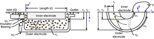
If one also assumes that the radius is nearly constant over the integral bounds (that is r_c ≫ r₂ – r₁, where r_c = (r₁ + r₂)/2 is the radius of the halfway point between the inner and outer electrode) and uses the definition of the average velocity, one can state (4) $$\Lambda =\frac{1}{2\delta \overline{v}{n}_0}\underset{r_1}{\overset{r_2}{\int }}n\left(r,L\right)v_z\mathrm{d}r,$$(4) where v̄ is the average axial velocity of the fluid through the device and δ = (r₂ – r₁)/2 is the half width of the gap between the inner and outer electrode. Determining the transfer function thus requires an estimate of n(r,L).

2.2. Governing physics

The number concentration of particles throughout the device is governed by the advective-diffusion equation (Olfert and Collings 2005), (5) $$\mathbf{v}\cdot \nabla n=D{\nabla }^{2}n-\nabla \cdot \mathbf{c}n,$$(5) where v = [v_r, v_θ, v_z]^T is the flow velocity field, where v_r, v_θ, and v_z are the velocity distribution in the radial, angular, and axial directions respectively; D is the diffusion coefficient; and c = [c_r, c_θ, c_z]^T is the particle migration velocity, with components assigned analogous to v. The particle migration velocity is the product of the net force on the nanoparticles and the mechanical mobility, B. The latter quantity can be defined in multiple ways, including (6) $$B=\frac{C_{\mathrm{c}}}{3\pi \mu d_{\mathrm{m}}}=\frac{Z_{\mathrm{p}}}{q}=\frac{\tau }{m},$$(6) where C_c is the Cunningham slip correction factor of a particle with mobility diameter, d_m; μ is the gas viscosity; Z_p is the particle electromobility; q = z_ke is the particle charge, which is the product of the integer charge state, z_k, and the elementary charge, e; τ is the particle relaxation time; and m is particle mass. The net force on the particles is assumed to be isolated to the radial direction such that c_z = 0, c_θ = 0, and (7) $$c_{\mathrm{r}}=B\left(F_{\mathrm{c}}-F_{\mathrm{e}}\right)=\frac{\tau }{m}\left(F_{\mathrm{c}}-F_{\mathrm{e}}\right),$$(7) which includes electrostatic, (8) $$F_{\mathrm{e}}=\frac{qV}{r\hspace{0.17em}\text{ln}\hspace{0.17em}\left(r_2/r_1\right)},$$(8) and centrifugal forces, (9) $$F_{\mathrm{c}}=\frac{m{v}_{\theta }^2}{r}.$$(9)

From Equation (7)(7) $$c_{\mathrm{r}}=B\left(F_{\mathrm{c}}-F_{\mathrm{e}}\right)=\frac{\tau }{m}\left(F_{\mathrm{c}}-F_{\mathrm{e}}\right),$$(7) , it becomes clear that particle mass analyzers in fact classify particles with respect to their mass-to-charge ratio. Going forward, a single integer charge will be assumed on the particles, z_k = 1, with other integer charge states receiving attention in Section S.5.6 of the online supplementary information (SI). Further, in these expressions, V refers to the setpoint voltage; (10) $$v_{\theta }={\omega }_1\frac{{\widehat{r}}^2-\widehat{\omega }}{{\widehat{r}}^2-1}r+{\omega }_1{r}_1^2\frac{\widehat{\omega }-1}{{\widehat{r}}^2-1}\frac{1}{r}=\alpha r+\frac{\beta }{r},$$(10) is the azimuthal velocity distribution (Olfert and Collings 2005; Taylor 1923); ω₁ is the rotational speed of the inner electrode; r̂ = r₁/r₂ is the ratio of the inner to the outer radius; $\widehat{\omega }$ = ω₂/ω₁ is the ratio of the rotational speed of the outer electrode to the inner electrode; and α and β are summary parameters describing the velocity distribution. The particle migration velocity can now be stated as (11) $$c_{\mathrm{r}}=\frac{\tau v_{\theta }^2}{r}-\frac{\tau q{V}_l}{mr\hspace{0.17em}\text{ln}\hspace{0.17em}\left(r_2/r_1\right)}=\tau {\alpha }^{2}r+\frac{2\tau \alpha \beta }{r}+\frac{\tau {\beta }^2}{r^3}-\frac{\tau qV}{mr\hspace{0.17em}\text{ln}\hspace{0.17em}\left(r_2/r_1\right)}=\tau {\alpha }^{2}r+\frac{2\tau \alpha \beta }{r}+\frac{\tau {\beta }^2}{r^3}-\frac{\tau C_0}{mr},$$(11) where (12) $$C_0=\frac{qV}{\hspace{0.17em}\text{ln}\hspace{0.17em}\left(r_2/r_1\right)}$$(12) is a summary parameter that will recur throughout this work. This quantity can be updated to incorporate multiply charged and uncharged particles, something considered further in Section S.5.6 of the SI. In the case that the rotational speeds of the inner and outer electrodes are the same, that is for an APM, this can be simplified to (13) $$c_{\mathrm{r}}=\tau {\omega }^{2}r-\frac{\tau C_0}{mr},$$(13) noting that α = ω under these conditions. Assuming a fully developed flow and invoking continuity gives v_r = 0. The axial flow distribution, v_z, is commonly assumed to be either constant across the domain, v_z = v̄, corresponding to a plug flow, or more accurately (given that the entrance length is generally a fraction of a millimeter) as parabolic, (14) $$v_{\mathrm{z}}=\frac{3\overline{v}}{2}\left(1-{\frac{\left(r-r_{\mathrm{c}}\right)}{{\delta }^2}}^2\right)\text{for}r\in \left[r_1,r_2\right].$$(14) where v̄ refers to the average flow velocity (Ehara, Hagwood, and Coakley 1996). The latter representation is more accurate, being derived from the Navier-Stokes equation for a viscous flow (Landau and Lifshitz 1987). Finally, it is noted that the device is rotationally symmetric, such that ∂n_i/∂θ = 0.

Expanding Equation (5)(5) $$\mathbf{v}\cdot \nabla n=D{\nabla }^{2}n-\nabla \cdot \mathbf{c}n,$$(5) and eliminating the components that are zero, (15) $$v_{\mathrm{z}}\frac{\partial n}{\partial z}=D\left(\frac{1}{r}\frac{\partial }{\partial r}\left(r\frac{\partial n}{\partial r}\right)+\frac{{\partial }^{2}n}{\partial z^2}\right)-\frac{1}{r}\frac{\partial r{c}_{\mathrm{r}}n}{\partial r}.$$(15)

Using the product rule and noting that axial diffusion is negligible compared to advection (large Peclet number), this expression can be further simplified to (16) $$v_{\mathrm{z}}\frac{\partial n}{\partial z}=D\left(\frac{{\partial }^{2}n}{\partial r^2}+\frac{1}{r}\frac{\partial n}{\partial r}\right)-\left(\frac{1}{r}\frac{\partial r{c}_{\mathrm{r}}}{\partial r}n+c_{\mathrm{r}}\frac{\partial n}{\partial r}\right)=D\frac{{\partial }^{2}n}{\partial r^2}+\left(\frac{D}{r}-c_{\mathrm{r}}\right)\frac{\partial n}{\partial r}-\frac{1}{r}\frac{\partial r{c}_{\mathrm{r}}}{\partial r}n.$$(16)

This expression cannot generally be solved analytically, requiring other approaches to evaluate the number density for use in the transfer function, Equation (4)(4) $$\Lambda =\frac{1}{2\delta \overline{v}{n}_0}\underset{r_1}{\overset{r_2}{\int }}n\left(r,L\right)v_z\mathrm{d}r,$$(4) .

3. Finite difference simulations of the number concentration

3.1. Solving for the number concentration

Olfert and Collings (2005) used a finite difference scheme to evaluate the number concentrations over the particle mass analyzer domain, limiting their consideration to an approximate representation of the particle migration velocity. As the number concentration is considered symmetric in the azimuthal direction, the domain is discretized into N_r by N_z annuli having widths in the radial and axial direction of Δr and Δz, respectively. The Crank-Nicholson algorithm is used to solve Equation (16)(16) $$v_{\mathrm{z}}\frac{\partial n}{\partial z}=D\left(\frac{{\partial }^{2}n}{\partial r^2}+\frac{1}{r}\frac{\partial n}{\partial r}\right)-\left(\frac{1}{r}\frac{\partial r{c}_{\mathrm{r}}}{\partial r}n+c_{\mathrm{r}}\frac{\partial n}{\partial r}\right)=D\frac{{\partial }^{2}n}{\partial r^2}+\left(\frac{D}{r}-c_{\mathrm{r}}\right)\frac{\partial n}{\partial r}-\frac{1}{r}\frac{\partial r{c}_{\mathrm{r}}}{\partial r}n.$$(16) , lending itself to the discretization (17) $${\zeta }_i\left(n_i^{k+1}-n_i^k\right)=\gamma \left(n_{i+1}^{k+1}-2n_i^{k+1}+n_{i-1}^{k+1}+n_{i+1}^k-2n_i^k+n_{i-1}^k\right)+\left({\kappa }_i-{\varphi }_i\right)\left(n_{i+1}^{k+1}-n_{i-1}^{k+1}+n_{i+1}^k-n_{i-1}^k\right)-{\eta }_i\left(n_i^{k+1}+n_i^k\right)$$(17) where ζ_i = v_z(r_i)/Δz, γ = D/(2Δr²), κ_i = D/(4r_iΔr), φ_i = c_r|_r=ri/(4Δr), and η_i = 1/(2r_i)·∂rc_r/∂r|_r=ri and i and k refer the i^th radial and k^th axial position, respectively. Unlike the work of Olfert and Collings (2005), the present work uses the exact representation of the particle migration velocity, that is we use Equation (13)(13) $$c_{\mathrm{r}}=\tau {\omega }^{2}r-\frac{\tau C_0}{mr},$$(13) directly. At the inner and outer electrodes, n(r₁,z) = 0 and n(r₂,z) = 0, which is necessary to ensure particles only diffuse into the wall at the electrodes, not equally away from and toward the wall (that is not a radial derivative of zero). The equations can be modified to incorporate this explicitly by setting n_i+1^k+1 = 0 and n_i+1^k = 0 for the inner electrode and n_i-1^k+1 = 0 and n_i-1^k = 0 for the outer electrode. This represents a scheme in which Equation (17)(17) $${\zeta }_i\left(n_i^{k+1}-n_i^k\right)=\gamma \left(n_{i+1}^{k+1}-2n_i^{k+1}+n_{i-1}^{k+1}+n_{i+1}^k-2n_i^k+n_{i-1}^k\right)+\left({\kappa }_i-{\varphi }_i\right)\left(n_{i+1}^{k+1}-n_{i-1}^{k+1}+n_{i+1}^k-n_{i-1}^k\right)-{\eta }_i\left(n_i^{k+1}+n_i^k\right)$$(17) can be rearranged to give a system of equations (18) $$\mathbf{A}{\mathbf{x}}^{k+1}={\mathbf{y}}^k,$$(18) where (19) $$y_i^k=\left(\gamma -{\kappa }_i+{\varphi }_i\right)n_{i-1}^k+\left({\zeta }_i-2\gamma -{\eta }_i\right)n_i^k+\left(\gamma +{\kappa }_i-{\varphi }_i\right)n_{i+1}^k\text{for}i\in \left[1,N_{\mathrm{r}}\right],$$(19) (20) $$x_i^{k+1}=n_i^{k+1}\text{for}i\in \left[1,N_{\mathrm{r}}\right],$$(20) and (21) $$\mathbf{A}=\left[\begin{array}{cccc}{d}_1& b_1& & 0\\ a_2& d_2& \ddots & \\ & \ddots & \ddots & b_{n-1}\\ 0& & a_n& d_n\end{array}\right]$$(21) is a square, tridiagonal matrix with diagonals of a_i = –γ + κ_i – φ_i, d_i = ζ_i + 2γ + η_i, b_i = –γ_i – κ_i + φ_i. Note that the matrix A is independent of the axial position and can be precomputed before iterating with Crank-Nicholson. As the system is tridiagonal, this system can be solved efficiently using the Thomas algorithm (Thomas 1949), which requires on the order of N_r calculations at each axial position considered. Figure S1 in the SI shows the finite difference solutions for the number concentrations in a CPMA and APM corresponding to settings given in Table 1. The code associated with this article (Sipkens, Olfert, and Rogak 2019) demonstrates such calculations.

Table 1. Constant settings used to demonstrate transfer function evaluation for the particle mass analyzer. The two values of $\widehat{\omega }$ vary depending on whether a CPMA or APM is considered. Properties are otherwise identical between the two cases. Dimensions correspond to a commercially-available CPMA (Cambustion).

Property	r1 (mm)	r2 (mm)	Q (m^3/s)	L (m)	Rm	$\widehat{\omega },$ APM	$\widehat{\omega },$ CPMA	T (K)	p (atm)
Value	60	61	5.0 × 10-6	0.2	10	1.0	0.9697	293	1.0

The significance of diffusion in the finite difference simulations can be assessed by considering a non-dimensional diffusion coefficient. Consider the ratio of the average particle residence time, L/v̄, to a representative average time to diffuse the gap half width, D/δ². This allows one to define a non-dimensional diffusion coefficient as (22) $$D_0=\frac{L}{\overline{v}{\delta }^2}D=\frac{L}{\overline{v}{\delta }^2}{k}_{\mathrm{B}}TB=\frac{L}{\overline{v}{\delta }^2}\frac{C_{\mathrm{c}}{k}_{\mathrm{B}}T}{3\pi \mu d_{\mathrm{m}}},$$(22) which is inversely proportional to the mobility diameter. If D₀ is much less than unity (generally if D₀ < 0.003, which corresponds to d_m > 120 nm in this work), diffusion will be negligible, which allows for simplification of the governing equation (see Section S.2.1 of the SI). In the other limit (D₀ > 2, which corresponds to d_m < 4 nm in this work), most of the particles have the opportunity to diffuse to the wall, such that the transfer function is effectively zero everywhere. This parameter is used throughout this work as an indication of the relative significance of diffusion for a given setpoint.

3.2. Calculating the transfer function

The transfer function can now be defined based on the number concentration at the outlet. With a discrete representation of the number concentration at the outlet, the transfer function can be defined by discretizing Equation (3)(3) $$\Lambda =\frac{{\int }_{r_1}^{r_2}n\left(r,L\right)v_{z}r\mathrm{d}r}{n_0{\int }_{r_1}^{r_2}{v}_{z}r\mathrm{d}r}.$$(3) , without having to invoke the approximation that the radius is relatively constant over the gap, (23) $$\Lambda =\frac{{\sum }_i^{N_{\mathrm{r}}}\frac{n\left(r_i,L\right)}{n_0}\cdot v_z\left(r_i\right)\cdot r_i\cdot {\left(\Delta r\right)}_i}{{\sum }_i^{N_{\mathrm{r}}}{v}_z\left(r_i\right)\cdot r_i\cdot {\left(\Delta r\right)}_i}.$$(23)

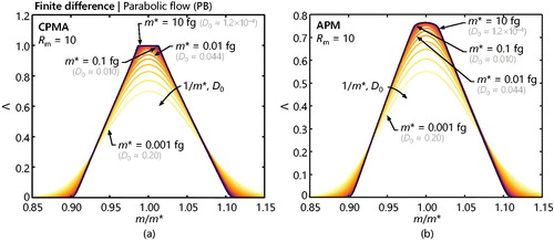
Figure 2 shows the transfer function for a range of setpoints, which are varied while holding an equivalent resolution (corresponding to the non-diffusing definition of Reavell, Symonds, and Rushton (2011) rather than the true full-width half-maximum, see Section S.3 of the SI for definition) constant at R_m = 10 and considering spherical particles with a density of ρ = 900 kg/m³. The remaining CPMA and APM properties are indicated in Table 1, differing only in the inner to outer electrode speed ratio, $\widehat{\omega },$ between the CPMA and APM settings. As expected, increased diffusion as the mobility size decrease changes the transfer function from a flat-top function to a Gaussian shape of increasing width. The functions otherwise share a common form. Under CPMA conditions, particles with specific properties are focused into a narrow region at the outlet (cf. Figure S1 showing number concentrations in the SI) such that those transfer functions with low amounts of diffusion allow for all of the particles within a specific range of setpoints to escape (Λ = 1). As the particle mobility decreases, some of these particles can diffuse to the wall, resulting in the peak of the transfer function holding values less than unity. At the same time, particles with different properties can diffuse into the center of the gap and exit the device, such that the transfer function widens. The shape of the APM transfer function is consistent with previous calculations by Ehara, Hagwood, and Coakley (1996) and Kuwata (2015) as discussed in the SI.

Figure 2. Transfer functions evaluated using the finite difference approach for a range of mass setpoints for a singly charged particle using a constant resolution, R_m = 10, and for spherical particles of a constant density, ρ = 900 kg/m³. The lines increment m* logarithmically with five values per decade and corresponds to particles with mobility diameters that range from 13 to 277 nm. Separate vertical scales are used for the CPMA and APM settings to accentuate the variation in each set of transfer functions. It is notable that the APM has lower particle transmission overall.

4. Non-diffusive particle tracking

Particle tracking techniques consider the trajectory of particles through the device as a function of the mass, integer charge state, electromobility, and device parameters (Ehara, Hagwood, and Coakley 1996; Stolzenburg 1988). This allows one to define a function, here denoted as G₀, that maps a particle’s final radial position to the radial position at the inlet, often allowing one to evaluate closed forms for the transfer function.

4.1. Procedure to evaluate the transfer function

4.1.1. Form of the transfer function

As per Section 2.1, the transfer function is defined as (24) $$\Lambda =\frac{1}{2\delta \overline{v}{n}_0}\underset{r_1}{\overset{r_2}{\int }}n\left(r,L\right)\cdot v_z\left(r\right)\cdot \mathrm{d}r.$$(24)

It is useful to change coordinate systems to the radial position of the particle at the inlet, where the number concentration is assumed to be uniform over the domain. By defining G₀(r) as the operator to map the final radial position of the particle to its position at the inlet, one can express the transfer function as (25) $$\Lambda =\frac{1}{2\delta \overline{v}{n}_0}{\int }_{G_0\left(r_1\right)}^{G_0\left(r_2\right)}n\left(r,0\right)\cdot v_z\left(r\right)\cdot \mathrm{d}r.$$(25)

Substituting Equation (2)(2) $$n\left(r,0\right)=n_0\left[H\left(r-r_1\right)-H\left(r-r_2\right)\right].$$(2) and canceling out n₀, (26) $$\Lambda =\frac{1}{2\delta \overline{v}}{\int }_{G_0\left(r_1\right)}^{G_0\left(r_2\right)}\left[H\left(r-r_1\right)-H\left(r-r_2\right)\right]\cdot v_z\left(r\right)\cdot \mathrm{d}r.$$(26)

Finally, the Heaviside function can be incorporated into the integral bounds, (27) $$\Lambda =\frac{1}{2\delta \overline{v}}\underset{r_{\mathrm{a}}}{\overset{r_{\mathrm{b}}}{\int }}{v}_z\left(r\right)\cdot \mathrm{d}r,$$(27) where (28) $$r_{\mathrm{a}}=\max \left\{r_1,\min \left\{r_2,G_0\left(r_1\right)\right\}\right\}=\min \left\{r_2,\max \left\{r_1,G_0\left(r_1\right)\right\}\right\}=\{\begin{array}{ll}{r}_1& G_0\left(r_1\right)\le r_1\\ G_0\left(r_1\right)& r_1<G_0\left(r_1\right)<r_2\\ r_2& G_0\left(r_1\right)\ge r_2\end{array}$$(28) and (29) $$r_{\mathrm{b}}=\min \left\{r_2,\max \left\{r_1,G_0\left(r_2\right)\right\}\right\}=\{\begin{array}{ll}{r}_1& G_0\left(r_2\right)\le r_1\\ G_0\left(r_2\right)& r_1<G_0\left(r_2\right)<r_2\\ r_2& G_0\left(r_2\right)\ge r_2\end{array}.$$(29) The piecewise representation, also shown in Equations (28)(28) $$r_{\mathrm{a}}=\max \left\{r_1,\min \left\{r_2,G_0\left(r_1\right)\right\}\right\}=\min \left\{r_2,\max \left\{r_1,G_0\left(r_1\right)\right\}\right\}=\{\begin{array}{ll}{r}_1& G_0\left(r_1\right)\le r_1\\ G_0\left(r_1\right)& r_1<G_0\left(r_1\right)<r_2\\ r_2& G_0\left(r_1\right)\ge r_2\end{array}$$(28) and (29)(29) $$r_{\mathrm{b}}=\min \left\{r_2,\max \left\{r_1,G_0\left(r_2\right)\right\}\right\}=\{\begin{array}{ll}{r}_1& G_0\left(r_2\right)\le r_1\\ G_0\left(r_2\right)& r_1<G_0\left(r_2\right)<r_2\\ r_2& G_0\left(r_2\right)\ge r_2\end{array}.$$(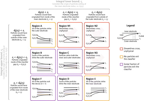29) , can be used to derive the transfer functions from Ehara, Hagwood, and Coakley (1996) and the analog for the other representations of the particle migration velocity (see Section S.5.3 of the SI for more detail). It also gives some intuition about the physical meaning of r_a, as the initial radius of a particle that will escape the classifier at the inner electrode, modified to return the closest of the inner and outer electrode radii when the particle would start outside of the classifier gap. The quantity r_b has an analogous meaning but for a particle that will escape the classifier closest to the outer electrode. This results in nine regions, identified in Figure 3, with letters reflecting those used by Ehara, Hagwood, and Coakley (1996) where possible. These bounds can also be represented in terms of absolute values to give a form similar to the transfer functions of Stolzenburg (2018) but for particle mass analyzers (again, see Section S.5.3 of the SI). The integral in Equation (27)(27) $$\Lambda =\frac{1}{2\delta \overline{v}}\underset{r_{\mathrm{a}}}{\overset{r_{\mathrm{b}}}{\int }}{v}_z\left(r\right)\cdot \mathrm{d}r,$$(27) can now be evaluated based solely on the chosen form for v_z, with simple analytical expressions possible for both the plug and parabolic flow conditions. Then, all that remains is to determine G₀.

Figure 3. The nine scenarios the particles could theoretically encounter in the classifier. Regions are lettered according to those regions originally identified by Ehara et al. (1996), where possible. Regions N1, N2, and N3 represent unphysical cases in that the particle streamlines cross. Regions A and E represent scenarios in which none of the particles will exit the device. Region F will only occur under CPMA conditions and represents the case where all of the particles of specific properties will exit the classifier. An estimate of where the equilibrium radius, r_s, will occur, when it exists, is also given in each panel.

4.1.2. Particle trajectories

The function G₀ can be determined by considering the motion of individual particles in the classifier that have an axial flow velocity, v_z, and a radial particle migration velocity, c_r. This relationship is described by an ordinary differential equation derived using chain rule, (30) $$\frac{\mathrm{d}r}{\mathrm{d}z}=\frac{\mathrm{d}r}{\mathrm{d}t}{\left(\frac{\mathrm{d}z}{\mathrm{d}t}\right)}^{-1}=\frac{c_{\mathrm{r}}}{v_{\mathrm{z}}}.$$(30)

This can be rearranged and integrated to define the function, (31) $$F\left(r\right)=\int \frac{v_{\mathrm{z}}}{c_{\mathrm{r}}}dr=z+c_1,$$(31) where c₁ is some constant that can be determined based on the starting radius of the particle. Defining r = r₀ at z = 0, then (32) $$c_1=F\left(r_0\right).$$(32)

The final radial position at z = L, r_L, is then related to the initial radial position by the relation (33) $$L=F\left(r_{\mathrm{L}}\right)-F\left(r_0\right).$$(33)

The operator G₀ is determined by rearranging Equation (33)(33) $$L=F\left(r_{\mathrm{L}}\right)-F\left(r_0\right).$$(33) to solve for r₀, (34) $$r_0=G_0\left(r_{\mathrm{L}}\right)=F^{-1}\left(F\left(r_{\mathrm{L}}\right)-L\right),$$(34) where F⁻¹ indicates the functional inverse of F. If the functional inverse cannot be evaluated analytically, one can estimate G₀(r_L) using a root-finding procedure, (35) $$G_0\left(r_{\mathrm{L}}\right)=\underset{r}{\mathrm{root}}\left\{F\left(r_{\mathrm{L}}\right)-F\left(r\right)-L\right\},$$(35) where $\underset{x}{\mathrm{root}}\left\{f(x)\right\}$ indicates the root of the function f(x) with respect to x. F and G₀ depend on one’s choice for both v_z and c_r, and a closed form expression for G₀(r) is only possible in select cases. However, in any case, with an estimate of G₀, the transfer function can be evaluated by substituting G₀ into Equations (28)(28) $$r_{\mathrm{a}}=\max \left\{r_1,\min \left\{r_2,G_0\left(r_1\right)\right\}\right\}=\min \left\{r_2,\max \left\{r_1,G_0\left(r_1\right)\right\}\right\}=\{\begin{array}{ll}{r}_1& G_0\left(r_1\right)\le r_1\\ G_0\left(r_1\right)& r_1<G_0\left(r_1\right)<r_2\\ r_2& G_0\left(r_1\right)\ge r_2\end{array}$$(28) and (29)(29) $$r_{\mathrm{b}}=\min \left\{r_2,\max \left\{r_1,G_0\left(r_2\right)\right\}\right\}=\{\begin{array}{ll}{r}_1& G_0\left(r_2\right)\le r_1\\ G_0\left(r_2\right)& r_1<G_0\left(r_2\right)<r_2\\ r_2& G_0\left(r_2\right)\ge r_2\end{array}.$$(29) to find r_a and r_b, respectively, and substituting these values into the result of the integral from Equation (27)(27) $$\Lambda =\frac{1}{2\delta \overline{v}}\underset{r_{\mathrm{a}}}{\overset{r_{\mathrm{b}}}{\int }}{v}_z\left(r\right)\cdot \mathrm{d}r,$$(27) for Λ.

4.2. Plug flow conditions (PL)

We proceed by first discussing G₀ for the plug flow condition and a range of representations of the particle migration velocity, before discussing the parabolic flow condition. Assuming a plug flow, v_z = v̄, the integral for the transfer function, Equation (27)(27) $$\Lambda =\frac{1}{2\delta \overline{v}}\underset{r_{\mathrm{a}}}{\overset{r_{\mathrm{b}}}{\int }}{v}_z\left(r\right)\cdot \mathrm{d}r,$$(27) , is straightforward: (36) $$\Lambda =\frac{r_{\mathrm{b}}-r_{\mathrm{a}}}{2\delta }.$$(36)

Programmatically, the simplest route to evaluating the transfer function is to substitute r_a and r_b (Equations (28)(28) $$r_{\mathrm{a}}=\max \left\{r_1,\min \left\{r_2,G_0\left(r_1\right)\right\}\right\}=\min \left\{r_2,\max \left\{r_1,G_0\left(r_1\right)\right\}\right\}=\{\begin{array}{ll}{r}_1& G_0\left(r_1\right)\le r_1\\ G_0\left(r_1\right)& r_1<G_0\left(r_1\right)<r_2\\ r_2& G_0\left(r_1\right)\ge r_2\end{array}$$(28) and (29)(29) $$r_{\mathrm{b}}=\min \left\{r_2,\max \left\{r_1,G_0\left(r_2\right)\right\}\right\}=\{\begin{array}{ll}{r}_1& G_0\left(r_2\right)\le r_1\\ G_0\left(r_2\right)& r_1<G_0\left(r_2\right)<r_2\\ r_2& G_0\left(r_2\right)\ge r_2\end{array}.$$(29) ) into this expression with the appropriate choice of G₀ (cf. Sections 4.2.1 through 4.2.5). However, some intuition can be gained by considering the piecewise definition of the bounds, which is considered further in Section S.5.3 of the SI. We now consider different realizations of G₀ for a range of functional forms for the particle migration velocity, with case codes assigned to represent the corresponding assumptions (see Table 2). In all of these cases, MATLAB functions that evaluate the transfer function by these various approaches are included both in a FigShare repository (Sipkens, Olfert, and Rogak 2019) and in a GitHub repository (https://github.com/tsipkens/mat-tfer-pma), with further details provided in the SI.

Table 2. Sequentially lettered cases for a range of representations of the particle migration velocity, c_r. The resultant functional forms for G₀ correspond to assuming a plug flow. A closed form is not available for Case GE.

Representation of the particle migration velocity	Case code	Functional form of cr	G0(rL), Plug flow (PL)
First-order Taylor series expansion about rs	1S*	$C_1(r-r_{\mathrm{s}})$	$r_{\mathrm{s}}+(r_{\mathrm{L}}-r_{\mathrm{s}})\hspace{0.17em}\text{exp}\hspace{0.17em}(-\lambda )$
First-order Taylor series expansion about rc	1C	$C_3+C_4(r-r_{\mathrm{c}})$	$r_{\mathrm{c}}+\left(r_{\mathrm{L}}-r_{\mathrm{c}}+\frac{C_3}{C_4}\right)\hspace{0.17em}\text{exp}\hspace{0.17em}\left(-\frac{C_{4}L}{\overline{v}}\right)-\frac{C_3}{C_4}$
Second-order Taylor series expansion about rs	2S	$C_1(r-r_{\mathrm{s}})+C_2{(r-r_{\mathrm{s}})}^2$	$r_{\mathrm{s}}+\frac{C_1(r-r_{\mathrm{s}})\hspace{0.17em}\text{exp}\hspace{0.17em}(-\lambda )}{C_2(r-r_{\mathrm{s}})+C_1-C_2(r-r_{\mathrm{s}})\hspace{0.17em}\text{exp}\hspace{0.17em}(-\lambda )}$
Second-order Taylor series expansion about rc	2C	$C_3+C_4(r-r_{\mathrm{c}})+C_5{(r-r_{\mathrm{c}})}^2$	$r_{\mathrm{c}}+\frac{f_1(r_{\mathrm{L}})/C_6-C_4}{2C_5}$
Exact for APM settings ($\widehat{\omega }$= 1)	W1	$\tau {\omega }^{2}r-\frac{\tau C_0}{mr}$	$\frac{1}{m^{1/2}\omega }{\left[(m{\omega }^2{r}_{\mathrm{L}}^2-C_0)\hspace{0.17em}\text{exp}\hspace{0.17em}(-\lambda )+C_0\right]}^{1/2}$
Exact, generalized expression	GE	$\tau {\alpha }^{2}r+\frac{2\tau \alpha \beta }{r}+\frac{\tau {\beta }^2}{r^3}-\frac{\tau C_0}{mr}$	Requires root-finding

* Case 1S corresponds to the case considered previously by Ehara et al. (1996). The resultant transfer function is identical when $\widehat{\omega }$= 1, with this work noting a minor correction that also allows for evaluation under CPMA conditions.

4.2.1. Case 1S-PL: First-order Taylor series approximation about the equilibrium radius

The simplest form of the problem is to approximate the particle migration velocity by a first-order Taylor series expansion. In the current state-of-the-art, the expansion is written about the equilibrium radius (Ehara, Hagwood, and Coakley 1996), r_s, such that (37) $$c_{\mathrm{r}}\approx C_1\left(r-r_{\mathrm{s}}\right),$$(37) where (38) $$C_1={\frac{\partial c_{\mathrm{r}}}{\partial r}|}_{r=r_{\mathrm{s}}}=\tau \left({\alpha }^2-\frac{2\alpha \beta }{r_{\mathrm{s}}^2}-\frac{3{\beta }^2}{r_{\mathrm{s}}^4}+\frac{C_0}{m{r}_{\mathrm{s}}^2}\right)=2\tau \left({\alpha }^2-\frac{{\beta }^2}{r_{\mathrm{s}}^4}\right).$$(38)

The equilibrium radius here is defined as the single radius at which particles of a specified mass and mobility will exit the device and will only exist under specific conditions (see Section S.4 of the SI for more information). When this approximation is used in Equation (31)(31) $$F\left(r\right)=\int \frac{v_{\mathrm{z}}}{c_{\mathrm{r}}}dr=z+c_1,$$(31) , F is given by (39) $$F\left(r\right)=\int \frac{\overline{v}}{C_1\left(r-r_{\mathrm{s}}\right)}dr=\frac{\overline{v}}{C_1}\text{ln}\hspace{0.17em}\left(r-r_{\mathrm{s}}\right)=\frac{L}{\lambda }\text{ln}\hspace{0.17em}\left(r-r_{\mathrm{s}}\right),$$(39) where the parameter (40) $$\lambda =\frac{L}{\overline{v}}\left[2\tau \left({\alpha }^2-{\beta }^2/r_{\mathrm{s}}^4\right)\right]$$(40) is often used to characterize a particle mass analyzer and determines the shape of the transfer function (Olfert and Collings 2005; Ehara, Hagwood, and Coakley 1996; Kuwata 2015). In this case, F is easily invertible, such that a closed form can be determined for G₀: (41) $$G_0\left(r_{\mathrm{L}}\right)=r_{\mathrm{s}}+\left(r_{\mathrm{L}}-r_{\mathrm{s}}\right)\hspace{0.17em}\text{exp}\hspace{0.17em}\left(-\lambda \right).$$(41)

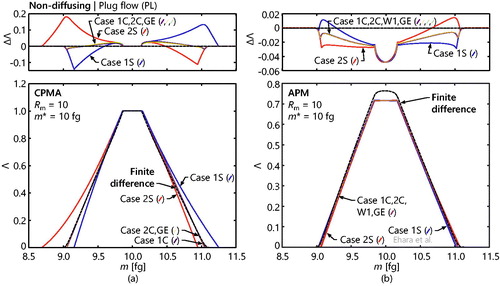
Figure 4 shows the transfer function resulting from this treatment for the CPMA and APM settings given in Table 1 and m* = 10 fg (corresponding to D₀ = 8.4 × 10⁻⁴, such that diffusion is negligible). In both cases, the transfer function exhibits the shape expected for a non-diffusing transfer function. For the CPMA setting, the predicted transfer function exhibits a mismatch against the finite difference solution in the wing regions where the Taylor series approximation fails because r_s is no longer contained in the gap. In contrast, for the APM setting, the predicted transfer function is well-represented in the wing regions but fails in the central region where the finite difference solution predicts a higher attenuation of particles and a non-linear dependence on mass. These characteristics are expected to result from a higher sensitivity to the axial flow distribution for the APM setting, where the particles are spread out over a larger region than for the CPMA setting. Despite this, the overall shape and width of the transfer function are reasonably predicted, even for the APM setting.

Figure 4. Realizations of the non-diffusing transfer function under plug flow conditions, for a (a) CPMA and (b) APM, and for a range of representations of the particle migration velocity (Cases 1S-PL through GE-PL). In each case, the transfer function is compared to the finite difference result (dashed line) with a low level of diffusion (m* = 10 fg and D₀ = 8.4 × 10⁻⁴). The top plots show the error between the predicted transfer functions and the finite difference solutions with a low level of diffusion. Different scales are used in each of the plots. A secondary peak was present for Case 2S-PL to the left of the current domain (centered about m = 7.3 fg). Separate vertical scales are used for the CPMA and APM settings to accentuate the variation in each set of transfer functions. Case 1S-PL for the APM corresponds to the plug flow transfer function given by Ehara et al. (1996). The finite difference solution is similar to that described by Olfert and Collings (2005), differing in that the previous work used a first-order Taylor series expansion about r_s to represent the particle migration velocity.

It is of note that when $\widehat{\omega }$ = 1, λ > 0 and this transfer function will converge to the one given by Ehara, Hagwood, and Coakley (1996). However, if $\widehat{\omega }$ ≠ 1, several discrepancies appear between the previous and current treatments. These differences are detailed in Section S.5.3 of the SI and serve as a caution to practitioners that Ehara et al.’s treatment cannot generally be extended to the CPMA, even if λ is updated. Evaluation can also be complicated by the fact that, theoretically, there can be two equilibrium radii (as detailed in Section S.4 of the SI), which can result in artificial peaks in the transfer function. Figure 5, which shows an estimate of the computational effort of the considered techniques, indicates that this approach (and similar approaches resulting in closed form expressions for the transfer function) is associated with a drop in computational effort of several orders of magnitude relative to the finite difference case.

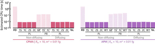
Figure 5. Estimated CPU time using the tic and toc functions in MATLAB for the various approaches of predicting the transfer function for m* = 0.01 fg. End cases correspond to the finite difference (FD) solution and the triangular approximation (Tri.), which is described further in Section S.6. Remaining cases correspond to evaluation of the particle tracking method across a range of representations of the particle migration velocity, axial flow conditions, and diffusion. Times are averaged over fifty runs. Note that these times should be considered relative to the other techniques, not as an indication of the absolute time associated with computation. Those bars indicated with a “*” do not have closed form solutions for G0, resulting in higher computational times relative to the other particle tracking approaches. Bars in darker colors correspond to preferred approaches from a computational effort perspective.

4.2.2. Case 1C-PL: First-order Taylor series approximation about the center radius of the gap

As the equilibrium radius will not always exist (see Section S.4 in the SI for additional details), alternate approaches must be considered to generalize transfer function evaluation. Accordingly, we also consider a Taylor series expansion about the center of the gap, r_c. This is a reasonable consideration as the integral for the transfer functions is only taken over the classifier gap. In this case, the Taylor series expansion becomes (42) $$c_{\mathrm{r}}\approx C_3+C_4\left(r-r_{\mathrm{c}}\right),$$(42) where (43) $$C_3={c_{\mathrm{r}}|}_{r=r_{\mathrm{c}}}=\tau \left({\alpha }^2{r}_{\mathrm{c}}+\frac{2\alpha \beta }{r_{\mathrm{c}}}+\frac{{\beta }^2}{r_{\mathrm{c}}^3}-\frac{C_0}{m{r}_{\mathrm{c}}}\right)$$(43) and (44) $$C_4={\frac{\partial c_{\mathrm{r}}}{\partial r}|}_{r=r_{\mathrm{c}}}=\tau \left({\alpha }^2-\frac{2\alpha \beta }{r_{\mathrm{c}}^2}-\frac{3{\beta }^2}{r_{\mathrm{c}}^4}+\frac{C_0}{m{r}_{\mathrm{c}}^2}\right).$$(44)

Note, that this includes an additional term in the Taylor series expansion relative to Case 1S-PL. Under this assumption, (45) $$F\left(r\right)=\frac{\overline{v}}{C_4}\text{ln}\hspace{0.17em}\left(C_4\left(r-r_{\mathrm{c}}\right)+C_3\right)$$(45) and (46) $$G_0\left(r_{\mathrm{L}}\right)=r_{\mathrm{c}}+\left(r_{\mathrm{L}}-r_{\mathrm{c}}+\frac{C_3}{C_4}\right)\hspace{0.17em}\text{exp}\hspace{0.17em}\left(-\frac{C_{4}L}{\overline{v}}\right)-\frac{C_3}{C_4}.$$(46)

Figure 4 also shows the transfer function resulting from this treatment for the CPMA and APM settings in Table 1 and m* = 10 fg. In general, the predicted transfer function is similar to that predicted for the Taylor series expansion about the equilibrium radius. For the CPMA setting, there is an improvement in the wing regions of the transfer function, with the overall width better reflecting the finite difference result (resulting in an order of magnitude improvement in the mean squared error, reported in Section S.5.7 of the SI, relative to the finite difference solution). This is expected to result from the fact that the particle migration velocity is better represented in these regions, where r_s lies outside of the gap. For the APM setting, the predicted transfer function is nearly identical to Case 1S-PL. Overall, then, this representation improves the estimates of the transfer function, while avoiding problems with the scenario in which r_s does not exist.

4.2.3. Cases 2S-PL and 2C-PL: Consideration of second-order Taylor series approximations

To improve the accuracy of the approximation to c_r, one could also consider a second-order Taylor series expansion. Closed form expressions are possible for G₀ when considering expansions about both r_s and r_c, with the resultant form of G₀ included in Table 2 and detailed further in Section S.5.4 of the SI. It is of note that while more accurate in the vicinity of r_s or r_c, larger errors are expected in the particle migration velocity away from r_s or r_c. As a result, the transfer functions can exhibit artificial peaks (which is present for Case 2S-PL to the left of the domain shown in Figure 4, centered about m = 7.3 fg). These extra peaks are a consequence of the numerical treatment of the problem, rather than properly representing the physics.

Figure 4 and the mean squared error reported in Section S.5.7 of the SI indicate that the Taylor series expansion about the equilibrium radius encounters a similar magnitude of error regardless of whether one considers the first- or second-order Taylor series approximation. For the CPMA setting, the width of the transfer function has in fact increased relative to Case 1S-PL, a consequence of larger errors in the Taylor series approximation as r_s moves out of the gap. The second-order Taylor series expansion about the center of the gap (Case 2C-PL) is visually indistinguishable from Case 1C-PL, indicating that there is little to no improvement to the transfer functions by including additional terms in the Taylor series expansion, while allowing the possibility of artificial peaks. Accordingly, it is recommended that second-order (or higher) Taylor series expansions be avoided.

4.2.4. Case W1-PL: Exact particle migration velocity for APM conditions

Consider now using the definition of the particle migration velocity under APM conditions, Equation (13)(13) $$c_{\mathrm{r}}=\tau {\omega }^{2}r-\frac{\tau C_0}{mr},$$(13) , (47) $$c_{\mathrm{r}}=\tau {\omega }^{2}r-\frac{\tau C_0}{mr}.$$(47)

When a plug flow is assumed, (48) $$F\left(r\right)=\frac{\overline{v}}{2\tau {\omega }^2}\text{ln}\hspace{0.17em}\left(m{\omega }^2{r}^2-C_0\right)$$(48) and (49) $$G_0\left(r_{\mathrm{L}}\right)=\frac{1}{m^{1/2}\omega }{\left[\left(m{\omega }^2{r}_{\mathrm{L}}^2-C_0\right)\hspace{0.17em}\text{exp}\hspace{0.17em}\left(-\lambda \right)+C_0\right]}^{1/2}.$$(49)

This form is relatively simple and indicates that Taylor-series expansions are not necessary for considering plug flow, non-diffusing, and APM conditions. Figure 4b shows the predicted transfer function for the APM setting. The result is nearly identical to Cases 1C-PL and 2C-PL, suggesting the validity of the first-order Taylor series expansion about the center of the gap. This also indicates that the remaining error in the central region of the transfer function is not a result of inaccuracies in the Taylor series approximation of the particle migration velocity but rather a sensitivity to the choice of axial flow conditions. Despite these inaccuracies, the result still improves the representation of the true transfer function relative to triangular approximations (cf. Section S.6 of the SI) without increasing the computational effort (cf. Figure 5).

4.2.5. Case GE-PL: Exact particle migration velocity for CPMA conditions

Finally, consider the definition of the particle migration velocity for general CPMA conditions, Equation (11)(11) $$c_{\mathrm{r}}=\frac{\tau v_{\theta }^2}{r}-\frac{\tau q{V}_l}{mr\hspace{0.17em}\text{ln}\hspace{0.17em}\left(r_2/r_1\right)}=\tau {\alpha }^{2}r+\frac{2\tau \alpha \beta }{r}+\frac{\tau {\beta }^2}{r^3}-\frac{\tau qV}{mr\hspace{0.17em}\text{ln}\hspace{0.17em}\left(r_2/r_1\right)}=\tau {\alpha }^{2}r+\frac{2\tau \alpha \beta }{r}+\frac{\tau {\beta }^2}{r^3}-\frac{\tau C_0}{mr},$$(11) , (50) $$c_{\mathrm{r}}=\tau {\alpha }^{2}r+\frac{2\tau \alpha \beta }{r}+\frac{\tau {\beta }^2}{r^3}-\frac{\tau C_0}{mr}.$$(50)

This results in (51) $$F=\frac{\overline{v}}{4\tau {\alpha }^2}[\text{ln}\hspace{0.17em}\left({\alpha }^2{r}^4+{\beta }^2+C_7{r}^2\right)-\frac{2C_7}{{\left(4{\alpha }^2{\beta }^2-C_7^2\right)}^{1/2}}{\hspace{0.17em}\text{tan}\hspace{0.17em}}^{-1}\left[\frac{2{\alpha }^2{r}^2+C_7}{{\left(4{\alpha }^2{\beta }^2-C_7^2\right)}^{1/2}}\right]],$$(51) where (52) $$C_7=2\alpha \beta -\frac{C_0}{m}.$$(52)

This function does not have a known functional inverse, requiring one to revert to a root-finding exercise to determine G₀. The complexity of this function makes root-finding challenging, particularly in that multiple zeroes and asymptotes can exist in the function. Accordingly, care must be taken to select the correct root. The interval in which the root occurs can be determined from a consideration of r_s. For example, if λ < 0 and r_s < r₁, then the correct root corresponding to G₀(r₁) will exist in the interval [r₁, ∞]. Similarly, if r_s > r₁, then the root corresponding to G₀(r₁) will exist in the interval [0, r₁]. It is worth noting that automated root-finding for this problem becomes impractical in cases where r_s does not exist, as the search interval is not well-defined. However, such cases are not encountered in the sample conditions used in the current work such that r_s can always be used to specify a search interval in which to look for a sign change. Figure 5 indicates that the root-finding procedure causes a significant increase in computation effort, making this approach disadvantageous relative to those cases where closed forms are available.

Figure 4 shows the predicted transfer function for this case. For the APM setting, the predicted transfer function is identical to Case W1-PL and is very similar to Cases 1C-PL and 2C-PL. For the CPMA, the predicted transfer function is also similar to that from Case 1C-PL and 2C-PL, again suggesting that the Taylor series expansion about the center of the gap is adequate for predicting the transfer function while reducing the overall computational effort.

4.3. Parabolic flow conditions (PB)

The axial flow profile inside the classifier is better represented by a parabolic flow (Landau and Lifshitz 1987). As a consequence, this condition is often considered in transfer function development, both in terms of the DMA and particle mass analyzers (e.g., Ehara, Hagwood, and Coakley 1996; Dubey and Dhaniyala 2008; Stolzenburg 2018). When the velocity is parabolic, Equation (14)(14) $$v_{\mathrm{z}}=\frac{3\overline{v}}{2}\left(1-{\frac{\left(r-r_{\mathrm{c}}\right)}{{\delta }^2}}^2\right)\text{for}r\in \left[r_1,r_2\right].$$(14) , the transfer function becomes (Ehara, Hagwood, and Coakley 1996) (53) $$\Lambda =\frac{3}{4\delta }\underset{r_{\mathrm{a}}}{\overset{r_{\mathrm{b}}}{\int }}\left[1-{\left(\frac{r-r_{\mathrm{c}}}{\delta }\right)}^2\right]\mathrm{d}r=\frac{3}{4}\left(\frac{r_{\mathrm{b}}-r_{\mathrm{a}}}{\delta }\right)-\frac{1}{4}\left[{\left(\frac{r_{\mathrm{b}}-r_{\mathrm{c}}}{\delta }\right)}^3-{\left(\frac{r_{\mathrm{a}}-r_{\mathrm{c}}}{\delta }\right)}^3\right].$$(53) where, as before, r_a and r_b depend on G₀. When considering a parabolic axial flow, closed forms for G₀ are not generally possible for any representation of the particle migration velocity in Table 2. Instead, every method here requires the use of the root-finding procedure, Equation (35)(35) $$G_0\left(r_{\mathrm{L}}\right)=\underset{r}{\mathrm{root}}\left\{F\left(r_{\mathrm{L}}\right)-F\left(r\right)-L\right\},$$(35) , to determine G₀. We note that second-order approximations were previously shown to be unnecessary and are not considered further here. We also note that a closed form is not possible even for the function F(r) in Case GE-PB. Evaluation of G₀ numerically would thus require the more general particle tracking method implemented by Hagwood et al. (1995) and Olfert (2005), albeit under different conditions. Due to the increased computational effort relative to the other approaches, this technique is also not considered further here.

4.3.1. Cases 1S-PB and 1C-PB: Consideration of first-order Taylor series approximations

For the first-order Taylor series approximations (Cases 1S-PB and 1 C-PB), F can still be expressed as a closed form, specifically as (54) $$F\left(r\right)=\frac{-3L}{2\lambda {\delta }^2}[\left(r_{\mathrm{s}}^2+r_{\mathrm{c}}^2-2r_{\mathrm{c}}{r}_{\mathrm{s}}-{\delta }^2\right)\hspace{0.17em}\text{ln}\hspace{0.17em}\left(r-r_{\mathrm{s}}\right)+\frac{r^2}{2}+\left(r_{\mathrm{s}}-2r_{\mathrm{c}}\right)r+2r_{\mathrm{c}}{r}_{\mathrm{s}}-\frac{3}{2}{r}_{\mathrm{s}}^2]$$(54) and (55) $$F\left(r\right)=\frac{-3\overline{v}}{4C_4^3{\delta }^2}\left[2\left(C_3^2-C_4^2{\delta }^2\right)\hspace{0.17em}\text{ln}\hspace{0.17em}\left(C_4\left(r-r_{\mathrm{c}}\right)+C_3\right)+C_4^2{\left(r-r_{\mathrm{c}}\right)}^2-2C_3{C}_4\left(r-r_{\mathrm{c}}\right)\right].$$(55) for expansions about r_s and r_c, respectively. The fact that a functional inverse of these expressions does not exist in terms of known functions is consistent with the findings of Ehara, Hagwood, and Coakley (1996). Also, as noted previously, problems can be encountered when applying a root-finding procedure in that there could be multiple zeroes in the function F(r_L) – F(r) – L and possible asymptotes. The search domain should again be restricted using r_s.

Figure 6 indicates the predicted transfer function for the CPMA and APM settings from Table 1 and for m* = 10 fg, using a root-finding procedure to determine G₀. For the CPMA setting, little improvement is observed relative to the plug flow case. The same is not true for the APM setting, where the discrepancy between the predicted transfer function and the finite difference solution has been almost entirely eliminated. This observation is reflected in the mean squared errors shown in Section S.5.7 of the SI. This affirms the former hypothesis that the axial flow condition was responsible for discrepancy observed in Figure 4b. Accordingly, use of the parabolic flow should be considered for cases where $\widehat{\omega }$ is very close to unity. This is helped by the fact that r_s will always exist under APM conditions, such that it is feasible to restrict the search domain considered during root-finding.

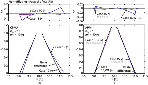
Figure 6. Realizations of the non-diffusing transfer function under parabolic flow conditions, for a (a) CPMA and (b) APM and for a range of representations of the particle migration velocity (Cases 1S-PB, 1C-PB, and W1-PB). In each case, the transfer function is compared to the finite difference result (dashed line) with a low level of diffusion (m* = 10 fg and D₀ = 8.4 × 10⁻⁴). Note that Case 1C-PL, that is the transfer function resulting from assuming plug flow as per Figure 4, is included in the APM panel for reference. The top plots show the error between the predicted transfer functions and the finite difference solutions with a low level of diffusion. Scales for each of these plots are the same as in Figure 4. Separate vertical scales are used for the CPMA and APM settings to accentuate the variation in each set of transfer functions. Case 1S-PB for the APM corresponds to the parabolic flow transfer function given by Ehara et al. (1996). Also note that the finite difference solutions presented here are identical to those given in Figure 4.

We note that one could consider approximating the logarithms in Equations (54)(54) $$F\left(r\right)=\frac{-3L}{2\lambda {\delta }^2}[\left(r_{\mathrm{s}}^2+r_{\mathrm{c}}^2-2r_{\mathrm{c}}{r}_{\mathrm{s}}-{\delta }^2\right)\hspace{0.17em}\text{ln}\hspace{0.17em}\left(r-r_{\mathrm{s}}\right)+\frac{r^2}{2}+\left(r_{\mathrm{s}}-2r_{\mathrm{c}}\right)r+2r_{\mathrm{c}}{r}_{\mathrm{s}}-\frac{3}{2}{r}_{\mathrm{s}}^2]$$(54) and (55)(55) $$F\left(r\right)=\frac{-3\overline{v}}{4C_4^3{\delta }^2}\left[2\left(C_3^2-C_4^2{\delta }^2\right)\hspace{0.17em}\text{ln}\hspace{0.17em}\left(C_4\left(r-r_{\mathrm{c}}\right)+C_3\right)+C_4^2{\left(r-r_{\mathrm{c}}\right)}^2-2C_3{C}_4\left(r-r_{\mathrm{c}}\right)\right].$$(55) using Taylor series expansions, where a second-order approximation produces terms of the same order as the remainder of the corresponding equations. The result is that the roots could theoretically be found using the quadratic formula, as demonstrated in Section S.5.5 of the SI. Unfortunately, Taylor series expansion of this form are divergent in the center region and inaccurate in the wing regions, making the resultant closed form expressions inaccurate.

4.3.2. Case W1-PB: Exact particle migration velocity for APM conditions

Given the definition of the particle migration velocity and the simplifications for APM conditions, F can be expressed as (56) $$F\left(r\right)=\frac{-3\overline{v}}{4\tau {\omega }^4{\delta }^2}[\left({\omega }^2\left(r_{\mathrm{c}}^2-{\delta }^2\right)+\frac{C_0}{m}\right)\hspace{0.17em}\text{ln}\hspace{0.17em}\left(\frac{C_0}{m}-{\omega }^2{r}^2\right)+4r_c\omega {\left(\frac{C_0}{m}\right)}^{1/2}{\tanh }^{-1}\left[{\left(\frac{m}{C_0}\right)}^{1/2}\omega r\right]+{\omega }^2\left(r^2-4r_{\mathrm{c}}r\right)].$$(56)

Using the root-finding procedure to determine G₀, Figure 6 shows that the resultant transfer function is indistinguishable from Case 1C-PB above (a fact reflected in the mean squared errors in Section S.5.7 of the SI). This again verifies that the first-order Taylor series approximation about the center of the gap is sufficient for defining the transfer function.

5. Particle tracking with diffusion

Diffusion can be added to the analysis of Section 4 by considering the movement of particles to adjacent trajectories. This can be represented by a convolution over the number concentration at the inlet, (57) $$n_{\mathrm{d}}\left(r_0,0\right)=\underset{-\infty }{\overset{\infty }{\int }}n\left(r,0\right)\cdot p\left(r_0,r\right)\cdot \text{dr},$$(57) where p(r₀,r) is a probability density function (pdf) weighting the number of particles about an initial radius, r, that will end up on the trajectory initiating at r₀ and n_d represents the corresponding effective number concentration of particles at the inlet. For diffusion, a natural choice for p(r₀,r) is Gaussian about r₀, that is (58) $$p\left(r_0,r\right)=\frac{1}{{\left(2\pi \right)}^{1/2}\sigma }\text{exp}\hspace{0.17em}\left[-\frac{1}{2}{\left(\frac{r_0-r}{\sigma }\right)}^2\right].$$(58)

The parameter σ is typically given as (Berg 1993; Hagwood et al. 1995) (59) $$\sigma ={\left(2DL/v_{\mathrm{z}}\right)}^{1/2},$$(59) which approximates the distance that a particle is expected to diffuse over the length of the device, relative to the gap width. This quantity will vary in the radial dimension due to the axial flow velocity, which is a consequence of particles diffusing farther in regions where the velocity is lower. Using Equation (2)(2) $$n\left(r,0\right)=n_0\left[H\left(r-r_1\right)-H\left(r-r_2\right)\right].$$(2) , the bounds on the integral in Equation (57)(57) $$n_{\mathrm{d}}\left(r_0,0\right)=\underset{-\infty }{\overset{\infty }{\int }}n\left(r,0\right)\cdot p\left(r_0,r\right)\cdot \text{dr},$$(57) can be adjusted, such that (60) $$n_{\mathrm{d}}\left(r_0,0\right)=n_0\underset{r_1}{\overset{r_2}{\int }}p\left(r_0,r\right)\cdot \mathrm{d}r.$$(60)

This can now be evaluated differently depending on one’s choice for the axial flow velocity. It is of note that this analysis ignores the fact that particles will diffuse to increasingly distant streamlines as the streamlines converge. This will correspond to a wider spread of particles with a given mass at the outlet relative to the particle tracking predictions. In other words, this corresponds to a larger opportunity for particles with properties away from the setpoint to diffuse towards the center (i.e., the true transfer function is higher away from the setpoint) and for particles typically near the center of the device to diffuse to the wall (i.e., the peak of the true transfer function is lower). This result in the true transfer function being wider than that predicted by this particle tracking method. The inverse is true if the streamlines diverge, resulting in the true transfer function being narrower than that predicted by this particle tracking method.

For a plug flow, v_z = v̄ is constant such that the integral in Equation (60)(60) $$n_{\mathrm{d}}\left(r_0,0\right)=n_0\underset{r_1}{\overset{r_2}{\int }}p\left(r_0,r\right)\cdot \mathrm{d}r.$$(60) can be evaluated as (61) $$n_{\mathrm{d}}\left(r_0,0\right)=\frac{n_0}{2}\left(\mathrm{erf}\left(\frac{r_0-r_2}{2^{1/2}\sigma }\right)-\mathrm{erf}\left(\frac{r_0-r_1}{2^{1/2}\sigma }\right)\right).$$(61)

This n_d(r₀,0) can then be substituted in the place of n(r,0) in Equation (25)(25) $$\Lambda =\frac{1}{2\delta \overline{v}{n}_0}{\int }_{G_0\left(r_1\right)}^{G_0\left(r_2\right)}n\left(r,0\right)\cdot v_z\left(r\right)\cdot \mathrm{d}r.$$(25) , such that (62) $$\Lambda =\frac{-1}{4\delta \overline{v}}{\int }_{G_0\left(r_1\right)}^{G_0\left(r_2\right)}\left(\mathrm{erf}\left(\frac{r-r_2}{2^{1/2}\sigma }\right)-\mathrm{erf}\left(\frac{r-r_1}{2^{1/2}\sigma }\right)\right)\cdot v_z\left(r\right)\cdot \mathrm{d}r.$$(62)

One can evaluate the integral as (63) $$\begin{array}{c}\Lambda =\frac{-1}{4\delta }{\int }_{G_0\left(r_1\right)}^{G_0\left(r_2\right)}\left(\mathrm{erf}\left(\frac{r-r_2}{2^{1/2}\sigma }\right)-\mathrm{erf}\left(\frac{r-r_1}{2^{1/2}\sigma }\right)\right)\cdot \mathrm{d}r\\ =\frac{-1}{4\delta }[\kappa \left(G_0\left(r_2\right),r_2\right)-\kappa \left(G_0\left(r_1\right),r_2\right)-\kappa \left(G_0\left(r_2\right),r_1\right)+\kappa \left(G_0\left(r_1\right),r_1\right)],\end{array}$$(63) where (64) $$\kappa \left(G_0\left(r_{\mathrm{g}1}\right),r_{\mathrm{g}2}\right)=\left(G_0\left(r_{\mathrm{g}1}\right)-r_{\mathrm{g}2}\right)\mathrm{erf}\left[\frac{G_0\left(r_{\mathrm{g}1}\right)-r_{\mathrm{g}2}}{2^{1/2}\sigma }\right]+\sigma {\left(\frac{2}{\pi }\right)}^{1/2}\hspace{0.17em}\text{exp}\hspace{0.17em}\left[-{\left(\frac{G_0\left(r_{\mathrm{g}1}\right)-r_{\mathrm{g}2}}{2^{1/2}\sigma }\right)}^2\right].$$(64)

In this case, the problem is now a matter of simple substitution of G₀ following the same procedure as that detailed in Section 4 (e.g., G₀(r) = r_s + (r_L – r_s)exp(–λ) for Case 1S-PL from Section 4.2.1).

When a parabolic velocity distribution is chosen, the problem becomes more challenging. Including a variable distance that the particles can diffuse, Equation (60)(60) $$n_{\mathrm{d}}\left(r_0,0\right)=n_0\underset{r_1}{\overset{r_2}{\int }}p\left(r_0,r\right)\cdot \mathrm{d}r.$$(60) becomes intractable. Alternatively, if one considers a uniform σ throughout the domain, considerable errors are encountered in the transfer function. For these reasons, this case is not considered further.

Figure 7 shows the effect of increasing the amount of diffusion (by decreasing the particle mass and mobility diameter) on the predicted transfer function assuming a plug flow and considering the first-order Taylor series approximation about the centerline radius (Case 1C-PL). As expected, the results closely resemble the finite difference solutions in Figure 1, affirming the treatment of diffusion proposed here as reasonable for plug flows. Similar observations were also obtained using the Monte Carlo approach by Hagwood et al. (1995). Figure 8 indicates the resultant transfer functions, assuming a plug flow and considering Cases 1S-PL through W1-PL, the cases for which closed form solutions are available for G₀. In general, the transfer functions for the CPMA matches the finite difference solutions (with mean squared errors reported in in Section S.5.7 of the SI). Case 2S does not decline to zero in the lower end of the domain due to the aforementioned, artificial peak that exists around m = 0.73 m*. For the APM setting, the predicted transfer functions underestimate the peak of the transfer function, a consequence of requiring parabolic axial flow conditions to accurately model the peak (as per Section 4).

Figure 7. Realizations of the diffusing transfer function under plug flow conditions for the CPMA setting from Table 1 and using a first-order Taylor series expansion about the centerline radius, r_c, for the particle migration velocity (Case 1C-PL). The lines increment m* logarithmically with five values per decade.

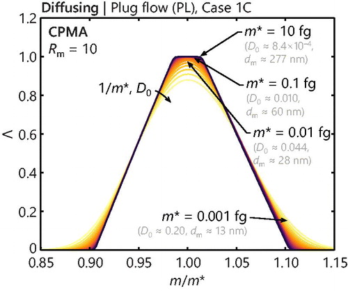
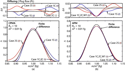
Figure 8. Realizations of the diffusing transfer function under plug flow conditions, for a (a) CPMA and (b) APM, and for a range of representations of the particle migration velocity (Cases 1S-PL through W1-PL). In each case, the transfer function is compared to the finite difference result (dashed line). The top plots show the error between the predicted transfer functions and the finite difference solutions. Scales for each of these plots are the same as in Figure 5, except for the plot containing the difference compared to the finite difference solution for (b). Separate vertical scales are used for the CPMA and APM settings to accentuate the variation in each set of transfer functions.

6. Conclusions

The current work examines a range of methods for evaluating the transfer function of particle mass analyzers, including the CPMA and APM. We first explicated the finite difference approach, which can evaluate the number concentration of particles throughout the device. This established method can visually demonstrate that the CPMA focuses particles of specific characteristics into narrow beams (see Section S.2.1 of the SI), while the APM suffers more significantly from particle losses. The resultant transfer function is used as a baseline for the other approaches discussed in this work.

We next present a framework that can be used to extend the previous particle tracking analysis of Ehara, Hagwood, and Coakley (1996) to consider a wider range of representations of the particle migration velocity, including exact representations and Taylor series approximations. Parabolic and plug axial flow conditions are considered. One’s choice of transfer function should depend on multiple factors:

1. The transfer function for the APM is highly sensitive to the axial flow conditions, while the transfer function for the CPMA is relatively independent of the axial flow conditions. As such, if diffusion is found to be negligible, one should consider using the parabolic forms of the transfer function for the APM but can retain the plug flow assumption for the CPMA. While this will incur a higher computational cost for the APM, the root-finding procedure is helped by the fact that r_s will always exist under these conditions such that the search domain can be restricted.

2. For the CPMA and when using the definition of the particle migration velocity without any approximations, G₀ can only be found by a root-finding procedure, which greatly increases CPU time. Therefore, it is recommended that one use the first-order Taylor series expansion about the center of the gap. This produces nearly identical transfer functions (see Section S.5.7 of the SI) while improving accuracy and avoiding problems about the existence of r_s relative to the case where expansions are taken about r_s (Ehara, Hagwood, and Coakley 1996).

3. If one is considering an APM without significant diffusion and wants fast computation, one should use Equation (49)(49) $$G_0\left(r_{\mathrm{L}}\right)=\frac{1}{m^{1/2}\omega }{\left[\left(m{\omega }^2{r}_{\mathrm{L}}^2-C_0\right)\hspace{0.17em}\text{exp}\hspace{0.17em}\left(-\lambda \right)+C_0\right]}^{1/2}.$$(49) (Case W1-PL) for G₀, which supersedes the previous function derived by Ehara, Hagwood, and Coakley (1996) in that it removes the need to use a Taylor series approximation. Practitioners should be aware that this will generally underestimate the peak because of the plug flow assumption.

4. Second-order Taylor series expansions should be avoided as they are prone to numerical artifacts, such as secondary peaks, and result in little or no improvement to the overall representation of the transfer function.

The cases where closed form expressions are available for the transfer function are summarized in Table 2 and in Section S.5.1 of the Supplemental Information. Implicit in these conclusions is the unintuitive result that the CPMA transfer functions are often easier to compute than APM transfer functions. This is a result of the CPMA transfer function being less sensitive to the axial flow conditions such that the closed form expressions for the plug flow conditions are reasonably accurate. This nearly voids the benefits of using triangular approximation of the transfer function, giving practitioners a model of similar computation effort and improved accuracy.

The above analysis is also extended to include diffusion in the transfer functions. Closed form expressions are often possible for plug flow conditions, while parabolic flow conditions require significant numerical effort and are not considered in this work. As plug flow conditions are sufficient for many CPMA settings, this presents a novel and simple way of computing transfer functions that include diffusion while significantly reducing the computational effort relative to the finite difference schemes used previously.

The present transfer functions can also be evaluated for the case of uncharged and multiply charged particles, as discussed in Section S.5.6 in the Supplemental Information.

Future work can use these new transfer functions to both speed up deconvolution of the instrument functions and further optimize device performance (e.g., following Tajima et al. (2011)).

Additional information

Funding

This work has been funded by the Natural Science and Engineering Research Council of Canada (2015-05905, PDF-516743-2018, FlareNet Research Network) and the Killam Foundation (Postdoctoral Fellowship).

References

- Beranek, J., D. Imre, and A. Zelenyuk. 2012. Real-time shape-based particle separation and detailed in situ particle shape characterization. Anal. Chem. 84 (3):1459–65.
- Berg, H. C. (ed.). 1993. Random walks in biology. In Diffusion: Microscopic theory, 5–16. Princeton: Princeton University Press.
- Bond, T. C., S. J. Doherty, D. W. Fahey, P. M. Forster, T. Berntsen, B. J. DeAngelo, M. G. Flanner, S. Ghan, B. Kärcher, D. Koch, et al. 2013. Bounding the role of black carbon in the climate system: A scientific assessment. J. Geophys. Res. Atmos. 118 (11):5380–552.
- Broda, K. N., J. S. Olfert, M. Irwin, G. P. Schill, G. R. McMeeking, E. G. Schnitzler, and W. Jäger. 2018. A novel inversion method to determine the mass distribution of non-refractory coatings on refractory black carbon using a centrifugal particle mass analyzer and single particle soot photometer. Aerosol Sci. Technol 52 (5):567–78. doi: 10.1080/02786826.2018.1433812.
- Charvet, A., S. Bau, N. E. P. Coy, D. Bémer, and D. Thomas. 2014. Characterizing the effective density and primary particle diameter of airborne nanoparticles produced by spark discharge using mobility and mass measurements (tandem DMA/APM). J. Nanoparticle Res. 16 (5):2418–28.
- Dubey, P., and S. Dhaniyala. 2008. Analysis of scanning DMA transfer functions. Aerosol Sci. Technol. 42 (7):544–55. doi: 10.1080/02786820802220258.
- Durdina, L., B. T. Brem, M. Abegglen, P. Lobo, T. Rindlisbacher, K. A. Thomson, G. J. Smallwood, D. E. Hagen, B. Sierau, and J. Wang. 2014. Determination of PM mass emissions from an aircraft turbine engine using particle effective density. Atmos. Environ. 99:500–7. doi: 10.1016/j.atmosenv.2014.10.018.
- Ehara, K., C. Hagwood, and K. J. Coakley. 1996. Novel method to classify aerosol particles according to their mass-to-charge ratio—Aerosol particle mass analyser. J. Aerosol Sci. 27 (2):217–34. doi: 10.1016/0021-8502(95)00562-5.
- Hagwood, C., K. Coakley, A. Negiz, and K. Ehara. 1995. Stochastic modeling of a new spectrometer. Aerosol Sci. Technol. 23 (4):611–27. doi: 10.1080/02786829508965342.
- Johnson, T. J., J. S. Olfert, R. Cabot, C. Treacy, C. U. Yurteri, C. Dickens, J. McAughey, and J. P. R. Symonds. 2014. Steady-state measurement of the effective particle density of cigarette smoke. J. Aerosol Sci. 75:9–16. doi: 10.1016/j.jaerosci.2014.04.006.
- Johnson, T. J., J. P. Symonds, and J. S. Olfert. 2013. Mass–mobility measurements using a centrifugal particle mass analyzer and differential mobility spectrometer. Aerosol Sci. Technol. 47 (11):1215–25. doi: 10.1080/02786826.2013.830692.
- Knutson, E. O., and K. T. Whitby. 1975. Aerosol classification by electric mobility: Apparatus, theory, and applications. J. Aerosol Sci. 6 (6):443–51. doi: 10.1016/0021-8502(75)90060-9.
- Kuwata, M. 2015. Particle classification by the tandem differential mobility analyzer–particle mass analyzer system. Aerosol Sci. Technol. 49 (7):508–20. doi: 10.1080/02786826.2015.1045058.
- Kuwata, M., and Y. Kondo. 2009. Measurements of particle masses of inorganic salt particles for calibration of cloud condensation nuclei counters. Atmos. Chem. Phys. 9 (16):5921–32. doi: 10.5194/acp-9-5921-2009.
- Lall, A. A., W. Rong, L. Mädler, and S. K. Friedlander. 2008. Nanoparticle aggregate volume determination by electrical mobility analysis: Test of idealized aggregate theory using aerosol particle mass analyzer measurements. J. Aerosol Sci. 39 (5):403–17. doi: 10.1016/j.jaerosci.2007.12.010.
- Landau, L. D., and E. M. Lifshitz. 1987. Fluid mechanics. 2nd ed. Toronto: Pergamon Press Canada Ltd.
- McMurry, P. H., X. Wang, K. Park, and K. Ehara. 2002. The relationship between mass and mobility for atmospheric particles: A new technique for measuring particle density. Aerosol Sci. Technol. 36 (2):227–38. doi: 10.1080/027868202753504083.
- Myhre, G., D. Shindell, F.-M. Bréon, W. Collins, J. Fuglestvedt, J. Huang, D. Koch, J.-F. Lamarque, D. Lee, B. Mendoza, et al. 2013. Anthropogenic and natural radiative forcing. In Climate change 2013: The physical science basis. Contribution of working group I to the fifth assessment report of the intergovernmental panel on climate change, ed. T. F. Stocker, et al., 659–740 Cambridge: Cambridge University Press.
- Olfert, J. S., M. Dickau, A. Momenimovahed, M. Saffaripour, K. Thomson, G. Smallwood, M. E. J. Stettler, A. Boies, Y. Sevcenco, A. Crayford, and M. Johnson. 2017. Effective density and volatility of particles sampled from a helicopter gas turbine engine. Aerosol Sci. Technol. 51 (6):704–14. doi: 10.1080/02786826.2017.1292346.
- Olfert, J. S. 2005. A numerical calculation of the transfer function of the fluted centrifugal particle mass analyzer. Aerosol Sci. Technol. 39 (10):1002–9. doi: 10.1080/02786820500380222.
- Olfert, J. S., and N. Collings. 2005. New method for particle mass classification—The couette centrifugal particle mass analyzer. J. Aerosol Sci. 36 (11):1338–52. doi: 10.1016/j.jaerosci.2005.03.006.
- Olfert, J. S., J. P. R. Symonds, and N. Collings. 2007. The effective density and fractal dimension of particles emitted from a light-duty diesel vehicle with a diesel oxidation catalyst. J. Aerosol Sci. 38 (1):69–82. doi: 10.1016/j.jaerosci.2006.10.002.
- Park, K., F. Cao, D. B. Kittelson, and P. H. McMurry. 2003. Relationship between particle mass and mobility for diesel exhaust particles. Environ. Sci. Technol. 37 (3):577–83. doi: 10.1021/es025960v.
- Pratsinis, S. E. 1998. Flame aerosol synthesis of ceramic powders. Prog. Energy Combust. Sci. 24 (3):197–219. doi: 10.1016/S0360-1285(97)00028-2.
- Reavell, K., J. P. R. Symonds, and M. G. Rushton. 2011. Simplified approximations to centrifugal particle mass analyser performance. Poster presented at the European Aerosol Conference, Manchester, UK, September 4.
- Scheckman, J. H., P. H. McMurry, and S. E. Pratsinis. 2009. Rapid characterization of agglomerate aerosols by in situ mass—Mobility measurements. Langmuir 25 (14):8248–54. doi: 10.1021/la900441e.
- Schmid, O., E. Karg, D. E. Hagen, P. D. Whitefield, and G. A. Ferron. 2007. On the effective density of non-spherical particles as derived from combined measurements of aerodynamic and mobility equivalent size. J. Aerosol Sci. 38 (4):431–43. doi: 10.1016/j.jaerosci.2007.01.002.
- Shin, W. G., G. W. Mulholland, S. C. Kim, J. Wang, M. S. Emery, and D. Y. H. Pui. 2009. Friction coefficient and mass of silver agglomerates in the transition regime. J. Aerosol Sci. 40 (7):573–87. doi: 10.1016/j.jaerosci.2009.02.006.
- Stolzenburg, M. R. 1988. An ultrafine aerosol size distribution measuring system. PhD diss., University of Minnesota.
- Sipkens, T. A., J. S. Olfert, and S. N. Rogak. 2019. MATLAB tools for PMA transfer function evaluation. doi: 10.5281/zenodo.3513260.
- Stolzenburg, M. R. 2018. A review of transfer theory and characterization of measured performance for differential mobility analyzers. Aerosol Sci. Technol. 52 (10):1194–218. doi: 10.1080/02786826.2018.1514101.
- Stolzenburg, M. R., and P. H. McMurry. 2008. Equations governing single and tandem DMA configurations and a new lognormal approximation to the transfer function. Aerosol Sci. Technol. 42 (6):421–32. doi: 10.1080/02786820802157823.
- Tajima, N., N. Fukushima, K. Ehara, and H. Sakurai. 2011. Mass range and optimized operation of the aerosol particle mass analyzer. Aerosol Sci. Technol. 45 (2):196–214. doi: 10.1080/02786826.2010.530625.
- Taylor, G. I. 1923. VIII. Stability of a viscous liquid contained between two rotating cylinders. Philos. Trans. R. Soc. London Ser. A. 223 (605-615):289–343. doi: 10.1098/rsta.1923.0008.
- Thomas, L. H. 1949. Elliptic problems in linear difference equations over a network. New York: Columbia University.