Particle formation from vapors emitted from glowing wires: Theory and experiments

Abstract

A coupled CFD-aerosol dynamics (CFD-AD) model is developed for the simulation of formation and growth characteristics of particles generated from glowing wires. The governing equations of the model include Navier-Stokes framework for the fluid flow and general dynamic equation for the aerosol particles. The formulation uniquely couples standard k-e scheme (including mass, momentum, energy and boundary layer equations) with aerosol dynamics equations (nucleation, coagulation, condensation and deposition) through residence time. Spatial and temporal characteristics of evolving aerosol spectrum can be simulated utilizing experimentally measured input parameters and wire compositional data. The coupling of CFD and aerosol dynamics offers better insights in comparison to standalone aerosol microphysics models. The results indicate that buoyancy effect is one of the key influencer in glowing wire systems. The CFD-AD was validated by comparing simulations with results obtained from six controlled experiments performed with a laboratory made hot wire nanoparticle generator. Condensation Particle Counter (CPC) and Scanning Mobility Particle Sizer (SMPS) were used for the measurement of total number concentration and number size distribution at the outlet of generator cell during these experiments. Model-predicted results were found to be following the trend of experimentally observed values. The developed model is computationally fast (fully implicit) and numerically stable. It can be used efficiently for studying the behavior of generated particles from glowing wires and other similar complex systems such as plasma torch aerosol generator, etc.

Copyright © 2019 American Association for Aerosol Research

Editor:

• Nicole Riemer

Introduction

Different methods are available to generate nanoparticle aerosols for laboratory purposes and industrial applications. These include generation from liquid phase via (Brust et al. 1994; Giersig and Mulvaney 1993), atomization of solutions (Yonezawa and Kunitake 1999; Boies et al. 2011a), crystallization of drops (Ranz et al. 1952) and generation in direct vapor phase (Sattler et al. 1980). The later includes phase change processes via furnace, flame, plasma, laser reactors, spark discharges and glowing wires (Khan et al. 2014; Jung et al. 2006; Jiang et al. 2004). In glowing wire technique, material is evaporated using a heated (glowing) wire and vapors are thermally quenched by a gas stream for nucleation (Nolan and Kennan 1948; O’Connor et al. 1959; O’Connor and Roddy 1966). A significant advantage of glowing/hot wire generator (HWG) is that it allows a precise control over the aerosol characteristics and contamination (Peineke et al. 2006, 2009). Owing to its exceptional characteristics, HWG has been used in past for different applications such as generating aerosol particles for surface coating (Boies et al. 2011b), as a particle size magnifier (Kangasluoma et al. 2013, 2015), etc. It is also used as a high number concentration source (Khan et al. 2014), as a calibrator of nanoparticle aerosol instruments (Hering et al. 2017), and for validation of aerosol dynamic (evolution) codes (Peineke and Schmidt-Ott 2008). Apart from core aerosol research, it finds application in diverse areas such as health (Zhang et al. 2005; Stark and Pratsinis 2002), combustion effects (Lin et al. 2005; Wang et al. 2017), aircraft emissions (Wong et al. 2008), environmental remediation (Zhang 2003), drug delivery (Cho et al. 2008) and contamination control (Gaborski et al. 2010).

The studies mentioned above were primarily performed to characterize particles generated from HWG, study their evolution dynamics and utilize the properties for various domains. Relatively fewer studies focused on the theoretical aspects related to HWG and the particles generated from HWG (Peineke et al. 2006; Jeon et al. 2003) are reported. Simulation of the generation process and the subsequent particle characteristics becomes challenging due to high temperatures, phase transition, dynamics in nuclei mode (<20 nm particle diameter) size ranges, spatial gradients and fast growth time-scales. In HWG and similar systems, dynamics of the bulk carrier and the suspended particles is interlinked due to the mass, momentum and energy transfer between the vapor and the particulate phase. Local thermodynamic conditions such as thermal gradients, convective and eddy currents, partial and saturation vapor pressure, condensational sinks, mixing efficiencies etc. affect the transfer mechanisms. These conditions are also linked with complex phenomena, e.g., entrainment fluid motion (vorticity of fluid, turbulence effects, etc.) having potential to perturb aerosol characteristics. It is a well-known fact that the aerosol parameters such as size, number concentration, polydispersity, structure and morphology are strongly coupled with the bulk fluid flow through residence time (Brown et al. 2006). Understanding of such interdependency is the first step towards characterizing and controlling the birth, life and fate of the nanoparticle aerosols. Any inaccuracy in quantifying the separate effects and the chained features may eventually lead to erroneous features in the system behavior. For systems involving two-phase processes, a coupled computational fluid dynamics- aerosol dynamics model can provide better insights than solving general dynamic equation adopting analytical (Lushnikov 1976) or numerical (Laakso et al. 2002) approach. Computational flow dynamics CFD techniques with limitations have been adopted in aerosol studies for 2 D (Lu et al. 1996; Nazaroff and Cass 1989; Adam et al. 1994; Stratmann and Whitby 1989) and 3 D cases (Nguyen et al. 2015). Lu et al. (1996) developed a CFD model for aerosol particle distribution in a ventilated chamber, without growth dynamics. Brown et al. (2006) studied heat and mass transfer effect on nucleation, coagulation and condensation process but did not study deposition which is important for closed systems. No efforts have been made to extend CFD methods for glowing wire systems possibly due to limited capability of commercial CFD codes for handling complex aerosol dynamics (Fluent 2009). As the lumped parameter approach cannot precisely handle spatial heterogeneity of process as well as aerosol parameters, CFD-aerosol coupling becomes quite applicable and relevant for HWG systems. Such coupling is capable of incorporating steep temperature gradients, fast time-scales, spatial heterogeneity in fluid parameters and deposition effects in framework of growth and evolution characteristics.

In this work, a CFD-AD model has been developed to simulate the characteristics of generated particles from HWG system. This model uses the spatial profile of temperature and flow velocity around the glowing wire and incorporates buoyancy effects and wall functions in the formulation. Dynamic implicit numerical scheme was used to solve mass, momentum and energy transfer in optimal time. Standard models for nucleation (Lai and Nazaroff 2000; Pirjola et al. 1999; Raes and Janssens 1986), condensation (Lai and Nazaroff 2000), coagulation (Lai and Nazaroff 2000; Vohra et al. 2017) and deposition (Crump and Seinfeld 1981) have been used. The developed model (CFD-AD) has been validated with results obtained from experiments performed in laboratory-made HWG (Khan et al. 2014). Grimm CPC and SMPS (Joshi et al. 2012) have been employed to measure time evolution of integral number concentration (≥4.5 nm) and size distribution (5–350 nm) at the outlet of HWG cell. Relevant input parameters (such as temperature of wire and surrounding space in glowing condition, wire characteristics, etc.) have been measured and used for simulations. This model, shown as a validated CFD coupled aerosol dynamics model abbreviated as CFD-AD, can be used as a standalone tool for hot wire generator (particle generation from glowing wires) and other similar complex applications.

Model description

This model (CFD-AD) couples $k-ϵ$ scheme with aerosol dynamics formulation adopted by Ghosh et al. (2017) and Lai and Nazaroff (2000). $k-ϵ$ turbulence scheme has been shown to be accurate for handling natural convection and buoyancy (Rincón-Casado et al. 2017) in past. Essential fluid properties, i.e., velocity, temperature, density, pressure and turbulent viscosity have been estimated for the fluid flow representing experimental conditions. Standard $k-ϵ$ framework has been modified to include buoyancy in convective scheme (Rincón-Casado et al. 2017). The combined model is then solved at each node of the mesh for each time step. The governing equations of the model are described below:

Mass balance equation

(1) $$\frac{\partial {\rho }_{\mathit{air}}}{\partial t}+\frac{\partial ({\rho }_{\mathit{air}}{u}_i)}{\partial x_i}=0$$(1)

Where x_i represents direction for X and Y, u_i represents corresponding velocities and ρ_air denotes the density of air.

Momentum equation

The equation representing conservation of momentum for the present context is modified by including buoyancy in the framework as follows (2) $$\frac{\partial ({\rho }_{\mathit{air}}{u}_i)}{\partial t}+\frac{\partial ({\rho }_{\mathit{air}}{u}_i{u}_j)}{\partial x_i}=-\frac{\partial P}{\partial x_i}+\frac{\partial }{\partial x_i}\left({\mu }_{\mathit{eff}}\frac{\partial u_i}{\partial x_i}\right)+{\rho }_{\mathit{air}}{g}_i$$(2)

where P is the system pressure (same as atmospheric pressure here), $g_i\approx g$ is the acceleration due to gravity Last term used in Equation (2)(2) $$\frac{\partial ({\rho }_{\mathit{air}}{u}_i)}{\partial t}+\frac{\partial ({\rho }_{\mathit{air}}{u}_i{u}_j)}{\partial x_i}=-\frac{\partial P}{\partial x_i}+\frac{\partial }{\partial x_i}\left({\mu }_{\mathit{eff}}\frac{\partial u_i}{\partial x_i}\right)+{\rho }_{\mathit{air}}{g}_i$$(2) accounts for the buoyancy force under constant gravity. Effective viscosity (μ_eff) used in Equation (2)(2) $$\frac{\partial ({\rho }_{\mathit{air}}{u}_i)}{\partial t}+\frac{\partial ({\rho }_{\mathit{air}}{u}_i{u}_j)}{\partial x_i}=-\frac{\partial P}{\partial x_i}+\frac{\partial }{\partial x_i}\left({\mu }_{\mathit{eff}}\frac{\partial u_i}{\partial x_i}\right)+{\rho }_{\mathit{air}}{g}_i$$(2) can be expressed as the sum of viscosity of air (μ) and turbulent viscosity (μ_t) quantifying the contribution of turbulence in flow. μ_t can be calculated from standard $k-ϵ$ equations as follows: (3) $${\mu }_t=\frac{{\rho }_{\mathit{air}}{C}_{\mu }{k}^2}{ϵ}$$(3) where $C_{\mu }$ is a constant value in standard $k-ϵ$ model taken as 0.09 (Mohammadi and Pironneau 1993), k of $k-ϵ$ model used is expressed as part of the following equation (4) $$\frac{\partial ({\rho }_{\mathit{air}}k)}{\partial t}+\frac{\partial ({\rho }_{\mathit{air}}k{u}_i)}{\partial x_i}=\frac{\partial }{\partial x_i}\left[\right(\mu +\frac{{\mu }_t}{{\sigma }_k}\left)\frac{\partial k}{\partial x_i}\right]+G_k+G_b-{\rho }_{\mathit{air}}ϵ$$(4) where σ_k is the constant term, with value equal to 1. G_k is the production of turbulent kinetic energy, which is a common term in all $k-ϵ$ models and G_b is the production of turbulent kinetic energy due to buoyant forces considering system is under a gravitation field (Rincón-Casado et al. 2017), described as (5) $$G_k=-{\rho }_{\mathit{air}}\overline{u_i^{\prime }}\overline{u_j^{\prime }}\frac{\partial u_j}{\partial x_i}$$(5) (6) $$G_b={\beta }_{th}{g}_i\left(\frac{{\mu }_t}{P{r}_t}\right)\frac{\partial T_{\mathit{air}}}{\partial x_i}$$(6) where $\overline{u_i^{\prime }}$ is the mean of the fluctuating velocity component of u_i. Pr_t is the turbulence Prandtl number, a dimensionless parameter expressing the ratio of momentum diffusivity to thermal diffusivity and is taken to be 0.72 (Rincón-Casado et al. 2017), T_air is the air temperature and β_th is the thermal expansion coefficient, described as (7) $${\beta }_{th}=-\frac{1}{{\rho }_{\mathit{air}}}\left(\frac{\partial {\rho }_{\mathit{air}}}{\partial x_i}\right)$$(7)

The ϵ equation of the standard $k-ϵ$ turbulence model is expressed as (8) $$\frac{\partial ({\rho }_{\mathit{air}}ϵ)}{\partial t}+\frac{\partial ({\rho }_{\mathit{air}}ϵu_i)}{\partial x_i}=\frac{\partial }{\partial x_i}\left[\right(\mu +\frac{{\mu }_t}{{\sigma }_{ϵ}}\left)\frac{\partial ϵ}{\partial x_i}\right]+G_k+{\rho }_{\mathit{air}}{C}_1{S}_{ϵ}+S_{ϵ}-\left(C_2{\rho }_{\mathit{air}}\frac{{ϵ}^2}{K}\right)+C_{1e}ϵ\left(\frac{G_k+C_{3e}{G}_b}{K}\right)$$(8) where $S_{ϵ}$ is the external source term and is optional. The ${\sigma }_{ϵ},$ C₁, C₂ and $C_{1ϵ}$ are constant terms in standard $k-ϵ$ model, with their values as 1.3, 0.44, 1.9 and 1.44, respectively (Wilcox et al. 1998; Rincón-Casado et al. 2017). The coefficient term $C_{3ϵ}$ can be calculated as follows (9) $$C_{3ϵ}=\tanh \left|\frac{u_j}{u_i}\right|$$(9)

Energy balance equation

Energy conservation equation for the present context has been written in terms of temperature as follows (10) $$\frac{\partial ({\rho }_{\mathit{air}}{T}_{\mathit{air}})}{\partial t}+\frac{\partial ({\rho }_{\mathit{air}}{u}_i{T}_{\mathit{air}})}{\partial x_i}=\frac{\partial }{\partial x_i}\left(\right(\frac{\mu }{Pr}+\frac{{\mu }_t}{P{r}_t}\left)\frac{\partial T_{\mathit{air}}}{\partial x_i}\right)+\frac{\partial Q_{\mathit{thi}}}{\partial t}$$(10) where T_air is the simulated air temperature and Q_th denotes the heat source term. For the case of heat generation due to electrical heating, Q_th can be calculated from the source-sink balance combining Joule’s law (Comte-Bellot 1976), convection loss (Comte-Bellot 1976) and radiation loss (Cohen and Glicksman 2015) described as (11) $$m_{\mathit{wire}}{c}_p\frac{\partial \mathit{Qth}}{\partial t}=I^2{R}_{\mathit{circuit}}-K_{\mathit{thermal}}{L}_{\mathit{wire}}\pi (T_{\mathit{wire}}-T_{\mathit{air}})NU-e_{\mathit{rad}}{\sigma }_{\mathit{rad}}{A}_{\mathit{wire}}(T_{\mathit{wire}}^4-T_{\mathit{air}}^4)$$(11)

In Equation (11)(11) $$m_{\mathit{wire}}{c}_p\frac{\partial \mathit{Qth}}{\partial t}=I^2{R}_{\mathit{circuit}}-K_{\mathit{thermal}}{L}_{\mathit{wire}}\pi (T_{\mathit{wire}}-T_{\mathit{air}})NU-e_{\mathit{rad}}{\sigma }_{\mathit{rad}}{A}_{\mathit{wire}}(T_{\mathit{wire}}^4-T_{\mathit{air}}^4)$$(11) the first term on the right-hand side is for the heat generated due to current flow in the circuit which was taken from the experimental conditions, the second term is for heat loss due to convection and the last term is for radiative heat loss to surroundings. In Equation (11)(11) $$m_{\mathit{wire}}{c}_p\frac{\partial \mathit{Qth}}{\partial t}=I^2{R}_{\mathit{circuit}}-K_{\mathit{thermal}}{L}_{\mathit{wire}}\pi (T_{\mathit{wire}}-T_{\mathit{air}})NU-e_{\mathit{rad}}{\sigma }_{\mathit{rad}}{A}_{\mathit{wire}}(T_{\mathit{wire}}^4-T_{\mathit{air}}^4)$$(11) I is for current, R is resistance of the circuit, K_thermal is thermal conductivity of wire material, L_wire is the length of the wire, m_wire is the wire mass, c_p is the specific heat capacity of wire material, T_wire is the wire temperature, e_rad is the radiation coefficient of the material, A_wire is the surface area of the wire and σ_rad is the Stefan-Boltzmann constant. The values of these parameters are given in the experimental section in Table 1. Nusselt number (NU) used in this equation was calculated for flat plate surface geometry (discussed in experimental section; Bodoia and Osterle 1962) as (12) $$NU=0.68+\frac{0.670{(R{a}_{\mathit{wire}})}^{1/4}}{{[1+{(\frac{0.492}{Pr})}^{9/16}]}^{4/9}}$$(12) where Ra_wire is the Raleigh number and can be described as (13) $$R{a}_{\mathit{wire}}=G{r}_{\mathit{wire}}Pr$$(13) where Gr_wire is the Grashof number for length of wire, described as (14) $$G{r}_{\mathit{wire}}=\frac{g{L}_{\mathit{wire}}(T_{\mathit{wire}}-T_{\mathit{air}})}{T_{\mathit{air}}{\mu }^2}$$(14)

Table 1. Parameters used for model calculation.

Item	Parameter name	Parameter value
Nichrome wire (in the form of a coil as shown in Figure 1)	Length	0.03 m
	Mass	0.0011 kg
	Inner diameter	0.011 m
	Input Power	10 & 30 W
	Specific heat capacity (cp)	450 J$k{g}^{-1}{K}^{-1}$
	Radiation coefficient (erad)	0.15 to 0.4 (Makino et al. 1982)
	Thermal conductivity (Kthermal)	2.5 $W{m}^{-1}{K}^{-1}$
	Stefan boltzmann constant (erad)	$5.6\times {10}^{-8}$ W$m^{-2}{K}^{-4}$
Chamber dimension	Length	0.12 m
	Height	0.06 m
Model input	Smallest grid size	1 mm
	Growth factor for grid size	1.05 (Rincón-Casado et al. 2017)
	Aerosol size bins	25, 50 and 100
	Aerosol size range	1 to 300 nm

For the case of 30 watt electrical power applied to the glowing wire, maximum Gr_wire is calculated to be approximately $1.6\times {10}^7;$ which is far higher than the estimated average Reynolds number (Re $\approx$ 424) in the computational domain. This indicates that only free convection can be considered as the major driving force for generating turbulence in the system (Bergman et al. 2011).

Equation for mass transfer

Vapor concentration profile (source term for aerosol formation) in the cell can be obtained by solving mass transfer, i.e., advection-diffusion equation which is shown below: (15) $$\frac{\partial ({\rho }_{\mathit{air}}C)}{\partial t}+\frac{\partial ({\rho }_{\mathit{air}}{u}_{i}C)}{\partial x_i}=(\frac{\mu }{Sc}+\frac{{\mu }_t}{Sc})\frac{{\partial }^{2}C}{\partial x_i^2}+C_{\mathit{source}}-I_{nu}{n}_{cr}$$(15)

In this equation, C specifies the concentration of vapor molecules emitted from the heated wire material and Sc denotes the Schmidt number. The last two terms on the right-hand side (RHS) are for vapor generation rate from the wire itself and loss rate due to nucleation process. Vapor source term (C_source) for this case was calculated by using Kays (2012) equation (16) $$C_{\mathit{source}}=\frac{K_{\mathit{conc}}(\mathit{Pvs}-P_{\mathit{surrounding}})}{R{T}_{\mathit{air}}}$$(16) where R is the gas constant, Pvs is a saturation vapor pressure of wire material (Alcock et al. 1984), P_surrounding is the partial vapor pressure and K_conc is the mass transfer coefficient in terms of Sherwood number (Sh), which can be expressed as (17) $$K_{\mathit{conc}}={\alpha }_{\mathit{conc}}Sh$$(17) where α_conc is the diffusion coefficient of the vaporized material. Sherwood number (Sh) used in above equation was calculated for the wire/flat surface from the following equation (18) $$Sh=0.664(R{e}^{0.5}S{c}^{1/3})$$(18) where Re is for Reynolds number which can be expressed as (19) $$Re=\frac{{\rho }_{\mathit{air}}u{L}_{\mathit{wire}}}{\mu }$$(19) where L_wire is the length of wire see Table 1 and u is the natural flow velocity.

General dynamics and transport equation of aerosol

In the most general form; aerosol formation, growth and transport in the cell volume (surface deposition included) can be mathematically expressed as (20) $$\begin{array}{c}\frac{\partial N(V,x,t)}{\partial t}+\frac{\partial u(x,t)N(V,x,t)}{\partial x}=(D{p}_l+{\mu }_t)\left[\frac{{\partial }^{2}N(V,x,t)}{\partial x^2}\right]+I_{nu}(x,t)n_{cr}(x,t)\\ +{\int }_0^{v}K{g}_{V-\overline{V},\overline{V}}^{x,t}N(V-\overline{V},x,t)N(\overline{V},x,t)d\overline{V}-{\int }_0^{\infty }K{g}_{V,\overline{V}}^{x,t}N(\overline{V},x,t)d\overline{V}-\lambda (V,x,t)N(V,x,t)\end{array}$$(20)

In above equation x represents direction, V is for volume of the particles and N represents number concentration. Second term in LHS and first term in RHS quantify aerosol transport due to advection and diffusion. Second term in RHS are for particle formation due to nucleation (Laakso et al. 2002). The next two terms are for particle coagulation (Ghosh et al. 2017; Vohra et al. 2017). In above formulation, Kg is the coagulation coefficient, n_cr is the critical number of molecules for nucleation. The numerical form of the above Equation (20)(20) $$\begin{array}{c}\frac{\partial N(V,x,t)}{\partial t}+\frac{\partial u(x,t)N(V,x,t)}{\partial x}=(D{p}_l+{\mu }_t)\left[\frac{{\partial }^{2}N(V,x,t)}{\partial x^2}\right]+I_{nu}(x,t)n_{cr}(x,t)\\ +{\int }_0^{v}K{g}_{V-\overline{V},\overline{V}}^{x,t}N(V-\overline{V},x,t)N(\overline{V},x,t)d\overline{V}-{\int }_0^{\infty }K{g}_{V,\overline{V}}^{x,t}N(\overline{V},x,t)d\overline{V}-\lambda (V,x,t)N(V,x,t)\end{array}$$(20) , (Pirjola et al. 1999; Raes and Janssens 1986) has been shown below Equation (21)(21) $$\begin{array}{c}\frac{\partial N_{i,l}}{\partial t}+\frac{\partial u_i{N}_{i,l}}{\partial x_i}=(D{p}_l+{\mu }_t)\left[\frac{{\partial }^2{N}_{i,l}}{\partial x_i^2}\right]+I_{nu}\frac{n_{cr}^i-n_{i,l-1}}{n_{i,l}-n_{i,l-1}}{f}_{n_{cr}^i,[n_{i,l-1},n_{i,l}]}+I_{nu}\frac{n_{i,l+1}-n_{cr}^i}{n_{i,l+1}-n_{i,l}}{f}_{n_{cr}^i,[n_{i,l},n_{i,l+1}]}\\ +\sum _{j=1}^l\sum _{k=j}^l\frac{K{g}_{j,k}^i}{1+{\delta }_{j,k}^i}{N}_{i,j}^t{N}_{i,k}^t-N_{i,l}^t\sum _{j=1}^{\mathit{nclass}}K{g}_{l,j}^i{N}_{i,j}^t-N_{i,l}^t{\lambda }_{i,l}\end{array}$$(21) . (21) $$\begin{array}{c}\frac{\partial N_{i,l}}{\partial t}+\frac{\partial u_i{N}_{i,l}}{\partial x_i}=(D{p}_l+{\mu }_t)\left[\frac{{\partial }^2{N}_{i,l}}{\partial x_i^2}\right]+I_{nu}\frac{n_{cr}^i-n_{i,l-1}}{n_{i,l}-n_{i,l-1}}{f}_{n_{cr}^i,[n_{i,l-1},n_{i,l}]}+I_{nu}\frac{n_{i,l+1}-n_{cr}^i}{n_{i,l+1}-n_{i,l}}{f}_{n_{cr}^i,[n_{i,l},n_{i,l+1}]}\\ +\sum _{j=1}^l\sum _{k=j}^l\frac{K{g}_{j,k}^i}{1+{\delta }_{j,k}^i}{N}_{i,j}^t{N}_{i,k}^t-N_{i,l}^t\sum _{j=1}^{\mathit{nclass}}K{g}_{l,j}^i{N}_{i,j}^t-N_{i,l}^t{\lambda }_{i,l}\end{array}$$(21)

where i represents directional coordinate for X and Y. j,k represent size classes of the coagulating particles and l represents the updated size after coagulation (j,k,l covering entire size range), nclass means the final size class of the size distribution, f is the delta function for the case of nucleation, similar to that of coagulation. The coagulation terms used in above equation also allows the interaction of monomer with l-mer. Kronecker’s delta function for the case of coagulation with respect to size can be described as (22) $${\delta }_{n_j+n_k,[n_l,n_{l+1}]}=\{\begin{array}{cc}0,\hfill & n_j+n_k\ne [n_l,n_{l+1}]\hfill \\ 1,\hfill & n_j+n_k=[n_l,n_{l+1}]\hfill \end{array}$$(22)

The last right hand side term of the Equation (21)(21) $$\begin{array}{c}\frac{\partial N_{i,l}}{\partial t}+\frac{\partial u_i{N}_{i,l}}{\partial x_i}=(D{p}_l+{\mu }_t)\left[\frac{{\partial }^2{N}_{i,l}}{\partial x_i^2}\right]+I_{nu}\frac{n_{cr}^i-n_{i,l-1}}{n_{i,l}-n_{i,l-1}}{f}_{n_{cr}^i,[n_{i,l-1},n_{i,l}]}+I_{nu}\frac{n_{i,l+1}-n_{cr}^i}{n_{i,l+1}-n_{i,l}}{f}_{n_{cr}^i,[n_{i,l},n_{i,l+1}]}\\ +\sum _{j=1}^l\sum _{k=j}^l\frac{K{g}_{j,k}^i}{1+{\delta }_{j,k}^i}{N}_{i,j}^t{N}_{i,k}^t-N_{i,l}^t\sum _{j=1}^{\mathit{nclass}}K{g}_{l,j}^i{N}_{i,j}^t-N_{i,l}^t{\lambda }_{i,l}\end{array}$$(21) is for wall deposition calculated using simulated velocity from $k-ϵ$ model, u_i, under the presence of gravity (Vohra et al. 2017). Particle diffusion coefficient (Dp) used above has been calculated from model temperature (T_air) and size of particles (d_p) (Rudyak 2013) as follows: (23) $$Dp=\frac{A+Q}{3\varphi }{N}_{AV}{\left(\frac{m_v}{2\pi }\right)}^{1/2}\frac{{(K{T}_{\mathit{air}})}^{3/2}}{{\rho }_{\mathit{air}}}\frac{1}{{(d_p)}^2}$$(23)

where $\varphi$ is a constant depending gas molecule interaction (Rudyak et al. 2009), N_AVis Avogadro’s number, d_p is the particle diameter and $(A+Q),$ the constant for modified Cunningham slip correction factor, described as (24) $$(A+Q)={(A+Q)}_0{\left(\frac{T_{\mathit{air}}}{T_0}\right)}^J$$(24) where ${(A+Q)}_0$ is the constant 1.657 and T₀ is 295, J is $\approx 1.6$ for particle diameter (d_p) less than $\approx 3.5$ nm and close to unity for particle diameter greater than $\approx 4$ nm.

Equation for aerosol formation (nucleation term)

The simulated temperature (T_air) and vapor concentration (C) distribution from fluid dynamics model have been used for calculating nucleation rate (I_nu) expressed as (25) $$I_{nu}=R_{ab}CZ\hspace{0.17em}\text{exp}\hspace{0.17em}\left(\frac{-\mathit{delG}}{K{T}_{\mathit{air}}}\right)$$(25) where R_ab is the average condensation rate (Laakso et al. 2002), Z is the zeldowich nonequilibrium factor (Laakso et al. 2002), K is for Boltzmann constant and delG is for nucleation barrier energy which can be expressed as (26) $$\mathit{delG}=\frac{-4\pi r_{\mathit{cri}}^{3}K{T}_{\mathit{air}}\hspace{0.17em}\text{log}\hspace{0.17em}S}{3v_{\mathit{mole}}}+4\pi \sigma r_{\mathit{cri}}^2$$(26) where v_mole is the molecular volume, σ is for surface tension of vaporized wire material (McNallan and Debroy 1991), S is the ratio between partial vapor pressure (P_surrounding) with saturation vapor pressure (Pvs) (Alcock et al. 1984) and r_cri is the critical radius of nucleating particles, generally this is taken as the first bin for the model. But, if the model predicted critical nucleation size is less than the molecular size of the evaporating material, then the molecular size is considered as the first bin. The r_cri can be described as (27) $$r_{\mathit{cri}}=\frac{2\sigma v_{\mathit{mole}}}{K{T}_{\mathit{air}}\hspace{0.17em}\text{log}\hspace{0.17em}S}$$(27)

The model framework discussed above is applicable for any aerosol generation and evolution context but specifically modified for the cases where particles are formed under glowing wire conditions (Burtscher et al. 1984; Magnusson et al. 1999; Müller et al. 1987, etc). These modifications pertain to the inclusion of buoyancy term in the Navier-Stokes Equation (2)(2) $$\frac{\partial ({\rho }_{\mathit{air}}{u}_i)}{\partial t}+\frac{\partial ({\rho }_{\mathit{air}}{u}_i{u}_j)}{\partial x_i}=-\frac{\partial P}{\partial x_i}+\frac{\partial }{\partial x_i}\left({\mu }_{\mathit{eff}}\frac{\partial u_i}{\partial x_i}\right)+{\rho }_{\mathit{air}}{g}_i$$(2) , source term in energy balance Equation (10)(10) $$\frac{\partial ({\rho }_{\mathit{air}}{T}_{\mathit{air}})}{\partial t}+\frac{\partial ({\rho }_{\mathit{air}}{u}_i{T}_{\mathit{air}})}{\partial x_i}=\frac{\partial }{\partial x_i}\left(\right(\frac{\mu }{Pr}+\frac{{\mu }_t}{P{r}_t}\left)\frac{\partial T_{\mathit{air}}}{\partial x_i}\right)+\frac{\partial Q_{\mathit{thi}}}{\partial t}$$(10) and vapor source dynamics (Section 2.4). The formulation calculates the values of governing parameters (temperature, density, vapor concentration) and can be used for studying spatial and temporal evolution of aerosol characteristics (number concentration, size distribution). The model was computationally simulated in Matlab parallel software (2016 version) and experimentally validated as a part of this work. All relevant parameters (system and process related) and constants used in the model are shown in Table 1.

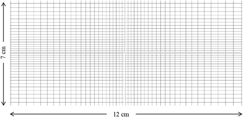
Model setup and numerical scheme

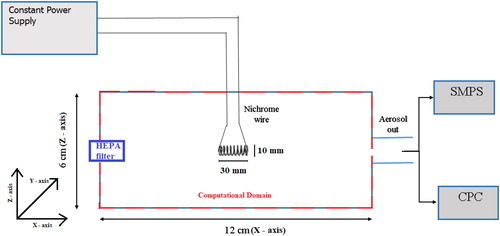
Numerical simulations for the present case were performed for 2 D geometry in order to reduce computational cost. This approximation is justified for the present case as the main flow is driven by natural convection (opposite to the direction of gravity). Experimental validation of temperature profile inside the HWG chamber also justified the 2-D approach. Approximating the case to 2 D fluid flow, fluid properties were estimated in X-Z plane and subsequently convoluted with aerosol dynamical equation at designated nodes (Lu et al. 1996). The physical problem considered in this work is a two-dimensional projection of a cylindrical chamber, made of stainless steel with length and diameter of 12 cm and 6 cm, respectively, which are of the same geometrical configuration as the one used in experiments (see Figure 1). Nichrome coil (0.1 mm diameter, 20 turns) used as vapor source was projected as a rectangular box (3 cm x 1 cm), source of heat for simulations. The chamber was divided into small variable grids with growth ratio 1.05. The minimum grid size was taken as 1 mm x 1 mm at the center of the chamber. With this configuration, meshes with proportional growth are achieved along with smaller discretization errors. The number of grids in the X and Y direction are varied depending on the size of the enclosure. Subsequently Navier-Stokes equations describing the fluid motion for a given set of boundary conditions were employed. These equations, along with the turbulence, energy equation and aerosol dynamics are solved at each grid of the mesh. All simulations were performed in absence of external forced flow (no guided flow except natural convection), similar to experimental measurements. This model couples $k-ϵ$ scheme for simulating turbulence in the bulk part with enhanced wall function model at the boundary layer. In order to obtained accurate numerical solution, meshing of the computational domain is an important step, specially for the boundary layer, where steep gradients in flow dynamics create a highly convective zone. For this reason, enhanced wall function (Rincón-Casado et al. 2017) has been shown to increase accuracy near the boundary layer. Radiation coefficient (specifying radiation loss of wire in glowing condition) was taken as 0.28–0.3 (Makino et al. 1982) The model simulations are performed for aerosol size distribution from 1 to 300 nm after performing grid independency tests for three different (25, 50, and 100) logarithm size bins. Results of grid independency test for one of the cases (30-watt power) have been demonstrated in Figure A3 (see Appendix).

Figure 1. Experimental setup.

Validation of model sections for limiting cases

As the combined model used in this work is complex and involves fluid as well as particle dynamics, it was important to validate sub-modules separately, by either taking specific cases or against published results. These sub-modules include particle nucleation, coagulation and deposition coupled with bulk fluid flow. Nucleation scheme used in the developed model was validated against results of the model discussed by Laakso et al. (2002). The formulations used for coagulation and aerosol deposition have also been validated in our previous work (Vohra et al. 2017; Ghosh et al. 2017). Modified $k-ϵ$ formulation after including buoyancy has been validated for the case discussed in Rincón-Casado et al. (2017). Grid independency test was performed for output variables viz. number concentration and number size distribution at the outlet of the generator. It was found that these variables changed by a maximum of 5% on reducing grid spacing by a factor of 10. So, grid size 1 mm with growth factor 1.05 was selected for simulations performed by using the developed model. This was in accordance with previously reported studies (Brown et al. 2006). A separate grid independency test for the standalone $k-ϵ$ module was also performed and the results are presented in the Appendix.

Experimental setup

Six experiments were performed in controlled conditions in HWG chamber. Figure 1 shows the schematic diagram of power supply set-up and instrumentation employed for aerosol particle generation and measurements. A constant power supply was used to maintain the power (10-, 20-, and 30-watt electrical power input) given to glowing wire. Temperature of the wire and the other regions of the chamber was measured in a separate series of experiments. K-type thermocouple was employed for these measurements and the obtained results were linked to the simulations. For comparison with model simulated results, GRIMM 5.403 condensation particle counter (CPC) (measuring aerosols having diameter larger than 4.5 nm) was used to measure integral aerosol number concentration, while GRIMM Scanning mobility particle sizer (SMPS) (5-350 nm in 45 size channels) was employed for measuring number size distribution. In addition, X-ray dispersion (XRD) techniques were utilized for determining the chemical characteristic of the wire, both before (unburnt) and after (burned) carrying out the experiment. One end of the generator was connected to CPC and SMPS for aerosol measurements and all other ports (not shown here) were connected with HEPA filters. Although HWG has provisions to transport generated particles using a carrier gas (air or any other working gas), this selection helped to focus on the role of buoyancy driven convective flows. One end of the generator was connected to CPC and SMPS for aerosol measurements while an excess port was used for flow balancing as shown in Figure 1.

Hot wire generator

The hot wire generator (Figure 1) consists of a metallic coil (1 mm diameter, 30 mm long, 20 turns) covered by stainless steel providing an interaction volume of 450 cm³ for the generated nanometer range metal aerosols. For the 2-D model approach, wire has been considered as a flat plate with equivalent length of 30 mm and height of 10 mm. The upper part of the generator was specially fabricated for electrical connection of the metal wire (handling currents in Ampere range) in the generator volume. A separate controller has been used to maintain fixed input power in the circuit. Horizontal sampling ports have been provided which may be used to guide the generated aerosols to the measuring equipment or to other larger experimental chambers. The specific chemical composition of the wire has been shown in the Appendix.

Results and discussion

Simulation of vapor and aerosol characteristics

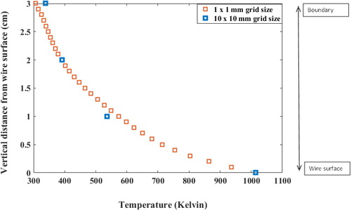
The developed CFD-AD model was used to calculate the essential characteristics of fluid flow namely velocity, temperature, density and viscosity. Accurate prediction of spatial temperature profile is crucial as it is directly linked to aerosol microphysical model, specifically for estimating nucleation rate profile in the chamber (Laakso et al. 2002; Pirjola et al. 1999). For the case of aerosol formation through electrically heated wire surface, temperature of the surface as well as nearby space is at significantly higher temperature compared to the other regions of the chamber. Such a scenario is expected to create nucleation zones where conversion of vapor to particle is highly probable. Further, the spatial temperature profile is also dependent on the buoyancy forces generated by temperature differences, for which Navier-Stokes (N-S) equation was modified by including $k-ϵ$ turbulent scheme (Rincón-Casado et al. 2017). As a first step, model simulated steady state temperature profile in the chamber was compared with the measured temperature during the experiments. Figure 2 compares the average spatial temperature profile generated from six controlled experiments with results obtained from simulations performed with respect to the experimental conditions (for all input electrical powers = 10, 20, and 30 watt).

Figure 2. Steady state spatial temperature profile in HWG cell: experimental measurements and simulations.

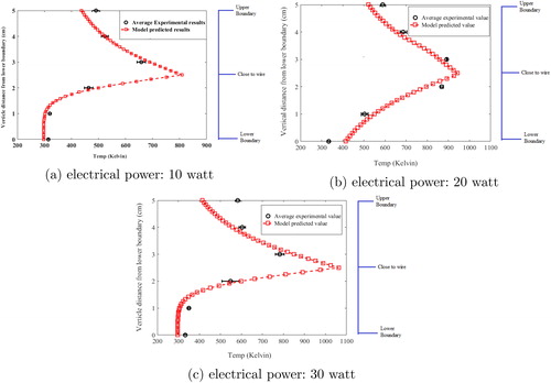
In Figure 2, average values for the measured temperature are plotted as black circles with error bars (one standard deviation), for the six experiments. The red squares denote the model simulated values. Temperature profile shown in this figure is for vertical line passing through the mid-plane of the glowing wire. The region around the wire has been divided into three sub-zones: upper boundary, close to wire and lower boundary, as shown in the above figure. Evidently, model predicted temperature values match well with the observed experimental data except at points near the upper boundary layer. The best correlation between simulated and experimental data is observed for the 10-watt case. The 30-watt results show relatively least correlation with experimental data, while 20-watt results are intermediate between the two. This is possibly due to the inaccuracies in the wall function used for the model in the turbulent convective zone. The effect is more pronounced for higher convection at 30-watt input power. The difference in temperature profile affects the vapor generation as shown in Figure 4. The heat accumulation in the upper boundary region resulted in non-homogeneous temperature distribution. This indicates that the upward convection due to the turbulence created by buoyancy is more significant than the heat diffusion (Rincón-Casado et al. 2017). Such a non-homogeneous distribution of temperature results in nucleation zones very close to the wire surfaces which may lead to rapid formation of aerosol particles (Herlach and Palberg 2016) of nano sizes in those zones.

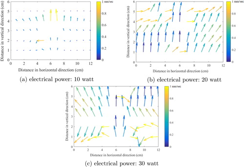
Figure 3 shows the model simulated steady state vapor velocity profile for all input power cases, viz. 10, 20, and 30 watts. All velocity profiles show that the buoyancy driven convection is the major source of velocity generation in HWG system. For the case of 10-watt input power, we observe weaker velocity field (mean velocity 0.12 mm/sec) compared to 20-watt input power (mean velocity 0.21 mm/sec) and 30-watt input power (mean velocity 0.27 mm/sec). An apparently distinct chaotic profile of fluid velocity distribution may have an impact on the aerosol dynamics, by influencing the particle transport, deposition and coagulation mechanisms.

Figure 3. Simulated steady state spatial velocity profile.

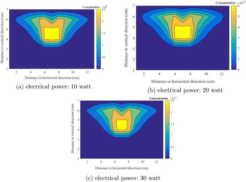
Apart from the temperature gradients and velocity profiles, which result in affecting vapor pressure and critical cluster size, source term of vapor molecules is also important for nucleation process. Therefore, it would be prudent to investigate vapor concentration profile without allowing nucleation process (Figure 4). This figure represents the steady state vapor concentration profile inside the chamber estimated from mass transfer Equation (15(15) $$\frac{\partial ({\rho }_{\mathit{air}}C)}{\partial t}+\frac{\partial ({\rho }_{\mathit{air}}{u}_{i}C)}{\partial x_i}=(\frac{\mu }{Sc}+\frac{{\mu }_t}{Sc})\frac{{\partial }^{2}C}{\partial x_i^2}+C_{\mathit{source}}-I_{nu}{n}_{cr}$$(15) ). Similar to the behavior of temperature inside the chamber, vapor profile also follows an upper region drift consequent to buoyant forces. The total vapor concentration reached up to $\approx {10}^8$ (10 watt case), $\approx {10}^{10}$ (20 watt case) and $\approx {10}^{12}$ (30 watt case) number of molecules $c{m}^{-3}.$ High vapor concentration can enhance the nucleation process significantly specially for 20- and 30-watt cases, leading to more nucleates. This leads to higher condensation and coagulation rates.

Figure 4. Steady state metal vapor concentration profile (inhibited nucleation conditions) inside the chamber.

In the next step, simulated vapor concentration profile was coupled with GDE model (Equation (21(21) $$\begin{array}{c}\frac{\partial N_{i,l}}{\partial t}+\frac{\partial u_i{N}_{i,l}}{\partial x_i}=(D{p}_l+{\mu }_t)\left[\frac{{\partial }^2{N}_{i,l}}{\partial x_i^2}\right]+I_{nu}\frac{n_{cr}^i-n_{i,l-1}}{n_{i,l}-n_{i,l-1}}{f}_{n_{cr}^i,[n_{i,l-1},n_{i,l}]}+I_{nu}\frac{n_{i,l+1}-n_{cr}^i}{n_{i,l+1}-n_{i,l}}{f}_{n_{cr}^i,[n_{i,l},n_{i,l+1}]}\\ +\sum _{j=1}^l\sum _{k=j}^l\frac{K{g}_{j,k}^i}{1+{\delta }_{j,k}^i}{N}_{i,j}^t{N}_{i,k}^t-N_{i,l}^t\sum _{j=1}^{\mathit{nclass}}K{g}_{l,j}^i{N}_{i,j}^t-N_{i,l}^t{\lambda }_{i,l}\end{array}$$(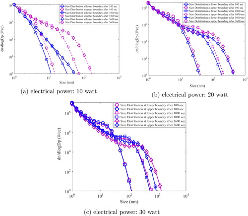21) )) and aerosol number characteristics were estimated for all size bins and all nodes as explained previously. Aerosol mobility sizer used in this work measured size distribution of particles from 5 nm to 300 nm. Hence simulation results for particle number concentration and size distribution were also obtained from 5 nm to 300 nm. Evolution of model simulated number size distribution for all input powers at different times (100, 1000 and 3600 s) for different regions of the chamber has been shown in Figures 5 and 6. These regions include two in horizontal direction (core and wall boundary) and two in vertical direction (lower and upper boundary).

Figure 5. Model simulated particle size distribution in two regions: core (close to wire) and wall boundary (close to measuring instruments) of the HWG system.

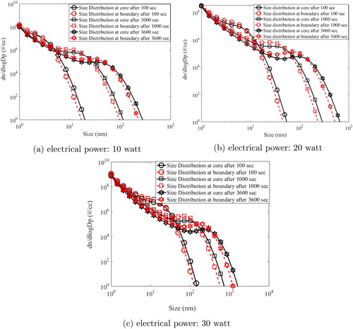
Figure 6. Model simulated particle size distribution in two regions (upper and lower boundary) of the HWG system.

In the above figure, grid average size distribution at the center of the chamber (core) is denoted as black squares while red circles denote the grid average size distribution at the wall boundary (close to measuring instruments). As the time progresses, aerosol size distribution evolves rapidly for all the cases. The shift in the mode is much higher for the case of 30 watts (Figure 5c) in comparison to 10 and 20 watts. While mode of particle size distribution (after 3600 s) at the boundary simulated for the case of 10 watt was $\approx 100$ nm, it was $\approx 1000$ nm for 30 watt input power. It is interesting to observe that the mode size at boundary increased almost 10 times when the input power increased 3 times. This is due to the increased growth rate from higher number of monomers resulting from high nucleation rate in 30-watt case. In addition, almost similar size distribution at the core and boundary at all times is noted. This indicates that the particles are well mixed. In similar direction, evolution of number concentration is also plotted at same time steps but for lower and upper boundary of HWG (Figure 6).

It can be seen from the above figure that number size distribution evolved significantly for 20- and 30-watt cases. For these powers, homogeneity of size distribution profile for both regions also signifies uniform mixing patterns. However, for the case of 10-watt power, buoyancy was seen to affect the aerosol dynamics. While number size distribution was found to be different at lower and upper boundary, the modal evolution with time was also different. This is due to the dominance of buoyant current transporting particles preferentially to the upper boundary. For higher powers, higher nucleation rate results in faster growth offsetting the transport of freshly formed particles to the upper boundary.

Comparison of model predictions and experimental observations

The experimental measurements for number concentration and number size distribution were performed at the outlet of the hot wire chamber (see Figure 1). Therefore, simulated results of only the boundary layer average grid (1 × 1 cm) close to outlet were used for this comparison. The time series of total number concentration of aerosol particles (4.5 nm to 300 nm size bins) for the three input power cases are shown in Figure 7.

Figure 7. Temporal evolution of total number concentration: experiments and simulations.

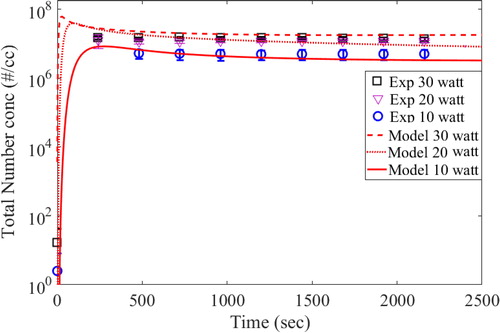
The red lines (solid and broken) in the above figure are drawn for the model predicted results for all three input power cases. Experimental results for 10, 20, and 30 watts have been averaged for six experiments performed for each case and have been shown as blue circle, purple triangle and black rectangle, respectively. Errors bars at one standard deviation are also plotted with these symbols in the figure. The number concentration at zero seconds (if any) is the background concentration of the system/chamber which exists before start of the experiments. As observed, model could predict the evolution of total number concentration reasonably well for all the cases. The difference noted for the initial times is due to the warm-up time taken by the wire before becoming red hot. Whereas the model assumes the wire to become instantly red hot, it took some time to reach that condition during measurements. However, profile measured by experiments was seen to follow the predicted trend after about 500 s. Total number concentration was also seen to be saturating for each case indicating the balance between the source rate and the depletion rate in small volume of the HWG cell. As a follow-up step, we also compared the number size distribution of the generated particles for all input powers, after 8 min and 1 h of the start of the glowing (shown in Figures 8 and 9, respectively).

Figure 8. Particle size distribution: model and experiments (after 8 min).

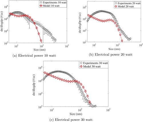
Figure 9. Particle size distribution: model and experiments (after 1 h).

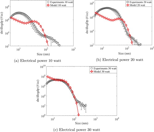
As can be seen for the case of input power as 10 watts (Figure 8a), model predictions are remarkably close to experimental values up to 100 nm particle diameter. For higher size ranges, model under-predicts the experimentally measured number size distribution. For 20-watt input power, model under-predicts the experimental results (Figure 8b). The comparison for the case of 30-watt input power yields mixed success wherein model can be seen to be close to experimental values for particle diameter lesser than 10 nm and higher than 60 nm (see Figure 8c). After 1 h, similar inferences but with overall better accuracy were obtained for the present context (Figure 9). The most probable reason accounting for the observed differences between model predictions and experimental measurements is the assumed spherical shape of the generated particles. Metal particles generated from HWG systems have been shown to possess fractal nature (Tsai et al. 1994) which may significantly modify the coagulation rates (Lee et al. 2000). In addition to shape factor induced inaccuracies, errors in the estimation of vapor emission rate (which was not measured experimentally due to limitations) may also contribute to differences (Peineke et al. 2006). Another aspect is related to the charge on the generated particles which also modifies the evolution dynamics (Ghosh et al. 2017). The current model treats particles as electrically neutral which may not be true. However, the model is successful in capturing the essential features and the coupling of CFD with aerosol dynamics paves the way for further improvements.

Conclusion

This work discusses the development of a model which can be used efficiently to study evolution of number concentration and size distribution of nanoparticles generated from glowing wire conditions. The developed model was tested against results obtained from experiments performed using hot wire generator. Incorporation of CFD in aerosol dynamics framework provides a realistic platform to study natural convection driven systems or applications. Aerosol dynamics sub-modules (nucleation, coagulation, wall deposition) have been coupled with Navier-Stokes equations modified to include buoyancy-coupled $k-ϵ$ turbulence model. Coupled flow-aerosol dynamics equation was solved numerically using implicit scheme. Measured wire composition and temperature (wire surface and cell domain) were used as input for the model simulations. Model simulations showed significant effect of fluid properties on the dynamics of aerosol particles. The role of buoyancy was highlighted by observation and interpretation of nucleation zones in the planes above the wire axis. The model was validated against measured temporal evolution of total number concentration and size distribution at the outlet of hot wire generator cell. Experimentally averaged and simulated total number concentrations were found to be closely matching, except at initial times. Steady state number size distribution matched very well for sub 10 nm particle diameters while reasonable differences were noticed for higher size ranges. Detailed CFD and aerosol dynamics for HWG system has been considered, however, there is scope for further improvement. Introduction of charge in aerosol dynamics (Ion-induced nucleation, charged particle coagulation, charged condensation and ion-induced deposition) and fractal dimension in coagulation model can be explored in future. Although tuned specifically for the present context (i.e., aerosol generation from hot wire generator), the model can also be used for diverse applications, e.g., emission of particles from hot zones (chimneys, exhaust), fires and atmospheric cloud dynamics.

Nomenclature
ρair	=	density of air
Awire	=	surface area of wire
C	=	vapor concentration
cp	=	specific heat capacity of wire material
delG	=	Gibbs free energy
Dpl	=	particle diffusion coefficient
erad	=	radiation coefficient
g	=	acceleration due to gravity
Gb	=	turbulent kinetic energy due to buoyancy force
Gk	=	turbulent kinetic energy
Grwire	=	Grashof number
I	=	circuit current
I nu	=	nucleation rate
K	=	Boltzmann constant
Kthermal	=	thermal conductivity
Kg	=	coagulation coefficient
l, j	=	size bins
mv	=	mass of gas molecule
mwire	=	mass of wire
N	=	aerosol concentration
N AV	=	Avogadro’s number
ncr	=	critical number for nucleation
Nsl	=	source of particles
NU	=	Nusselt number
P	=	chamber pressure
Psurrounding	=	partial vapor pressure
Pr	=	Prandtl number
Prt	=	turbulent Prandtl number
Pvs	=	saturation vapor pressure
Qth	=	source of heat
R	=	gas constant
Rab	=	average condensation rate
Rcircuit	=	resistance of the circuit
rcri	=	critical radius
Rawire	=	Raleigh number
Re	=	Reynolds number
S	=	saturation ration
Sc	=	Schmidt number
Sh	=	Sherwood number
Tair	=	air temperature
Twire	=	hot wire temperature
u	=	flow velocity
vmole	=	molecular volume of wire material

Greek letters
βth	=	thermal expansion coefficient
${\delta }_{l,m},{\delta }_{l+m,Q}$	=	Kronecker delta function with respect to charges
μ	=	air viscosity
μeff	=	effective viscosity
μt	=	turbulent viscosity
αconc	=	diffusion coefficient
λl	=	particle deposition rate
σ	=	surface tension
σrad	=	Stefan-Boltzmann constant

Appendix

Grid independency test for $k-ϵ$

model: Mesh structure used for simulations performed in computational domain has been shown in Figure A1. As can be observed, variable mesh sizing (more meshes near the wire) was adopted for simulations.

Figure A1. Mesh of the computational domain.

For performing grid independency, we performed a standalone model simulation of our $k-ϵ$ model for upper part of the hot wire generator (which is more important for natural convection). Results are shown in Figure A2. As can be seen, temperature values changed lesser than 5% corresponding to the decrease of grid spacing by a factor of 10.

Figure A2. Simulated temperature profile (grid independency).

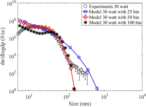
Size bin sensitivity test has been performed for the developed model for several cases and a representative result has been shown in Figure A3. This figure compares the number size distribution (10 watt input power, after 1 h of operation) measured during experiments with model simulations predicted for three different bin sizes viz. 25, 50, and 100 bins representing entire size distribution. It can be inferred that results were found to be independent of bin size for higher number of bins (50 and 100). The model simulations presented in this work used bin size of 100 covering number size distribution from 4.5 to 300 nm.

Figure A3. Size bin sensitivity test for 30 watt case.

Chemical composition of wire

The specific chemical composition (single or composite) of the wire can be determined through Energy Dispersive X-ray Spectroscopy (EDS) analysis (Kanda 1991) which had been used as an input parameter (calculating vapor production rate) of the coupled model. In the present work, nichrome wire was used for generating metal aerosol, and both EDS and XRD results indicate same metal composition. Figure A4a shows the EDS image of the section of wire which was used to obtain wire composition in terms of weight percentage of it’s components. Figure A4b represents the EDS spectrum of the wire section. The estimated weight percentages of wire components corresponding to EDS image have been shown in Table A1.

Figure A4. Image of the wire and the corresponding EDS spectrum.

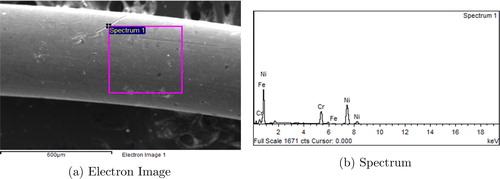
Table A1. Percentage of metal composition for experimental wire.

Metal composition	Weight percentage
Cr	21.33%
Ni	78.66%
Fe	0.01%

Acknowledgments

The authors are thankful to Pallavi Khandare and Amruta Nakhwa for providing help during experiments. They are also indebted to Professor Pratim Biswas for his support in the correction of the manuscript.

Additional information

Funding

The present study was supported in part by Health, Safety and Environmental group, Bhabha Atomic Research Center, Government of India. The authors gratefully acknowledge the financial support provided by Board of Research in Nuclear Science (BRNS), Department of Atomic Energy (DAE), Government of India to conduct this research under project no. 36(2,4)/15/01/2015-BRNS.

References

- Adam, N., K. Cheong, S. Riffat, and L. Shao. 1994. Measurement and modelling of aerosol particle flow in an environmental chamber. In Document-air infiltration Centre AIC PROC, 625. Oscar Faber Plc.
- Alcock, C., V. Itkin, and M. Horrigan. 1984. Vapour pressure equations for the metallic elements: 298–2500k. Canadian Metallurg. Quart. 23 (3):309–13. doi:10.1179/cmq.1984.23.3.309.
- Bergman, T. L., F. P. Incropera, D. P. DeWitt, and A. S. Lavine. 2011. Fundamentals of heat and mass transfer. Hoboken, NJ: John Wiley & Sons.
- Bodoia, J., and J. Osterle. 1962. The development of free convection between heated vertical plates. J. Heat Transfer 84 (1):40–3. doi:10.1115/1.3684288.
- Boies, A. M., P. Lei, S. Calder, and S. L. Girshick. 2011. Gas-phase production of gold-decorated silica nanoparticles. Nanotechnol. 22 (31):315603. doi:10.1088/0957-4484/22/31/315603.
- Boies, A. M., P. Lei, S. Calder, W. G. Shin, and S. L. Girshick. 2011. Hot-wire synthesis of gold nanoparticles. Aerosol Sci. Technol. 45 (5):654–63. doi:10.1080/02786826.2010.551145.
- Brown, D. P., E. I. Kauppinen, J. K. Jokiniemi, S. G. Rubin, and P. Biswas. 2006. A method of moments based CFD model for polydisperse aerosol flows with strong interphase mass and heat transfer. Computers Fluids 35 (7):762–80. doi:10.1016/j.compfluid.2006.01.012.
- Brust, M., M. Walker, D. Bethell, D. J. Schiffrin, and R. Whyman. 1994. Synthesis of thiol-derivatised gold nanoparticles in a two-phase liquid–liquid system. J. Chem. Soc., Chem. Commun. (7):801–2. doi:10.1039/C39940000801.
- Burtscher, H., A. Schmidt-Ott, and H. C. Siegmann. 1984. Photoelectron yield of small silver and gold particles suspended in gas up to a photon energy of 10 ev. Zeitschrift für Phys. B. Condensed Matter. 56 (3):197–9. doi:10.1007/BF01304172.
- Cho, K., X. Wang, S. Nie, Z. Chen, and D. M. Shin. 2008. Therapeutic nanoparticles for drug delivery in cancer. Clin. Cancer Res. 14 (5):1310–6. doi:10.1158/1078-0432.CCR-07-1441.
- Cohen, E., and L. Glicksman. 2015. Thermal properties of silica aerogel formula. J. Heat Transfer 137 (8):081601. doi:10.1115/1.4028901.
- Comte-Bellot, G. 1976. Hot-wire anemometry. Annu. Rev. Fluid Mech. 8 (1):209–31. doi:10.1146/annurev.fl.08.010176.001233.
- Crump, J. G., and J. H. Seinfeld. 1981. Turbulent deposition and gravitational sedimentation of an aerosol in a vessel of arbitrary shape. J. Aerosol Sci. 12 (5):405–15. doi:10.1016/0021-8502(81)90036-7.
- Fluent, A. 2009. 12.0 Theory guide. Ansys Inc, 5.
- Gaborski, T. R., J. L. Snyder, C. C. Striemer, D. Z. Fang, M. Hoffman, P. M. Fauchet, and J. L. McGrath. 2010. High-performance separation of nanoparticles with ultrathin porous nanocrystalline silicon membranes. ACS Nano. 4 (11):6973–81. doi:10.1021/nn102064c.
- Ghosh, K., S. Tripathi, M. Joshi, Y. Mayya, A. Khan, and B. Sapra. 2017. Modeling studies on coagulation of charged particles and comparison with experiments. J. Aerosol Sci. 105:35–47. doi:10.1016/j.jaerosci.2016.11.019.
- Giersig, M., and P. Mulvaney. 1993. Preparation of ordered colloid monolayers by electrophoretic deposition. Langmuir 9 (12):3408–13. doi:10.1021/la00036a014.
- Hering, S. V., G. S. Lewis, S. R. Spielman, A. Eiguren-Fernandez, N. M. Kreisberg, C. Kuang, and M. Attoui. 2017. Detection near 1-nm with a laminar-flow, water-based condensation particle counter. Aerosol Sci. Technol. 51 (3):354–62. doi:10.1080/02786826.2016.1262531.
- Herlach, D. M., and T. Palberg. 2016. Experimental studies of crystal nucleation: metals and colloids. arXiv Preprint arXiv:1605.03511
- Jeon, I.-D., M. Barnes, D.-Y. Kim, and N. M. Hwang. 2003. Origin of positive charging of nanometer-sized clusters generated during thermal evaporation of copper. J. Crystal Growth 247 (3–4):623–30. doi:10.1016/S0022-0248(02)02058-4.
- Jiang, H., S. Manolache, A. C. L. Wong, and F. S. Denes. 2004. Plasma-enhanced deposition of silver nanoparticles onto polymer and metal surfaces for the generation of antimicrobial characteristics. J. Appl. Polymer Sci. 93 (3):1411–22. doi:10.1002/app.20561.
- Joshi, M., B. Sapra, A. Khan, S. Tripathi, P. Shamjad, T. Gupta, and Y. Mayya. 2012. Harmonisation of nanoparticle concentration measurements using GRIMM and TSI scanning mobility particle sizers. J. Nanoparticle Res. 14 (12):1268. doi:10.1007/s11051-012-1268-8.
- Jung, J. H., H. C. Oh, H. S. Noh, J. H. Ji, and S. S. Kim. 2006. Metal nanoparticle generation using a small ceramic heater with a local heating area. J. Aerosol Sci. 37 (12):1662–70. doi:10.1016/j.jaerosci.2006.09.002.
- Kanda, K. 1991. Energy dispersive x-ray spectrometer. US Patent 5,065,020.
- Kangasluoma, J., M. Attoui, H. Junninen, K. Lehtipalo, A. Samodurov, F. Korhonen, N. Sarnela, A. Schmidt-Ott, D. Worsnop, M. Kulmala, and T. Petäjä. 2015. Sizing of neutral Sub 3 nm tungsten oxide clusters using airmodus particle size magnifier. J. Aerosol. Sci. 87:53–62. doi:10.1016/j.jaerosci.2015.05.007.
- Kangasluoma, J., H. Junninen, K. Lehtipalo, J. Mikkilä, J. Vanhanen, M. Attoui, M. Sipilä, D. Worsnop, M. Kulmala, and T. Petäjä. 2013. Remarks on ion generation for CPC detection efficiency studies in Sub-3-nm size range. Aerosol. Sci. Technol. 47 (5):556–63. doi:10.1080/02786826.2013.773393.
- Kays, W. M. 2012. Convective heat and mass transfer. Tata McGraw-Hill Education.
- Khan, A., P. Modak, M. Joshi, P. Khandare, A. Koli, A. Gupta, S. Anand, and B. Sapra. 2014. Generation of high-concentration nanoparticles using glowing wire technique. J. Nanoparticle Res. 16 (12):2776. doi:10.1007/s11051-014-2776-5.
- Laakso, L., J. M. Mäkelä, L. Pirjola, and M. Kulmala. 2002. Model studies on ion-induced nucleation in the atmosphere. J. Geophys. Res.: Atmospheres 107(D20):4427. doi:10.1029/2002JD002140.
- Lai, A. C., and W. W. Nazaroff. 2000. Modeling indoor particle deposition from turbulent flow onto smooth surfaces. J. Aerosol. Sci. 31 (4):463–76. doi:10.1016/S0021-8502(99)00536-4.
- Lee, D. G., J. S. Bonner, L. S. Garton, A. N. Ernest, and R. L. Autenrieth. 2000. Modeling coagulation kinetics incorporating fractal theories: a fractal rectilinear approach. Water Res. 34 (7):1987–2000. doi:10.1016/S0043-1354(99)00354-1.
- Lin, C.-C., S.-J. Chen, K.-L. Huang, W.-I. Hwang, G.-P. Chang-Chien, and W.-Y. Lin. 2005. Characteristics of metals in nano/ultrafine/fine/coarse particles collected beside a heavily trafficked road. Environ. Sci. Technol. 39 (21):8113–22. doi:10.1021/es048182a.
- Lu, W., A. T. Howarth, N. Adam, and S. B. Riffat. 1996. Modelling and measurement of airflow and aerosol particle distribution in a ventilated two-zone chamber. Building Environ. 31 (5):417–23. doi:10.1016/0360-1323(96)00019-4.
- Lushnikov, A. 1976. Evolution of coagulating systems: Iii. coagulating mixtures. J. Colloid Interface Sci. 54 (1):94–101. doi:10.1016/0021-9797(76)90288-5.
- Magnusson, M. H., K. Deppert, J.-O. Malm, J.-O. Bovin, and L. Samuelson. 1999. Gold nanoparticles: production, reshaping, and thermal charging. J. Nanoparticle Res. 1 (2):243–51. doi:10.1023/A:1010012802415.
- Makino, T., H. Kawasaki, and T. Kunitomo. 1982. Study of the radiative properties of heat resisting metals and alloys:(1st report, optical constants and emissivities of nickel, cobalt and chromium). Bull. JSME 25 (203):804–11. doi:10.1299/jsme1958.25.804.
- McNallan, M., and T. Debroy. 1991. Effect of temperature and composition on surface tension in Fe-Ni-Cr alloys containing sulfur. MTB. 22 (4):557–60. doi:10.1007/BF02654294.
- Mohammadi, B., and O. Pironneau. 1993. Analysis of the k-epsilon turbulence model.
- Müller, U., A. Schmidt-Ott, and H. Burtscher. 1987. First measurement of gas adsorption to free ultrafine particles: O 2 on ag. Phys. Rev. Lett. 58 (16):1684. doi:10.1103/PhysRevLett.58.1684.
- Nazaroff, W. W., and G. R. Cass. 1989. Mathematical modeling of indoor aerosol dynamics. Environ. Sci. Technol. 23 (2):157–66. doi:10.1021/es00179a003.
- Nguyen, T., A. Gerboud, and F. Garnier. 2015. 3D-modelling and simulation of thermodynamic process and aerosol precursors transformations in high-pressure turbine (hpt) of an aircraft engine with different operating conditions.
- Nolan, P. J., and E. Kennan. 1948. Condensation nuclei from hot platinum: size, coagulation coefficient and charge-distribution. In Proceedings of the Royal Irish Academy. Section A: Mathematical and Physical Sciences, 171–90. JSTOR.
- O’Connor, T., and A. Roddy. 1966. The production of condensation nuclei by heated wires. J. Rech. Atmos. 2:239–44.
- O’Connor, T., W. Sharkey, and C. O’Brolchain. 1959. On condensation nuclei produced at heated surfaces. Geofisica pura e applicata 42 (1):109–16. doi:10.1007/BF02113395.
- Peineke, C., M. Attoui, R. Robles, A. Reber, S. Khanna, and A. Schmidt-Ott. 2009. Production of equal sized atomic clusters by a hot wire. J. Aerosol. Sci. 40 (5):423–30. doi:10.1016/j.jaerosci.2008.12.008.
- Peineke, C., M. Attoui, and A. Schmidt-Ott. 2006. Using a glowing wire generator for production of charged, uniformly sized nanoparticles at high concentrations. J. Aerosol. Sci. 37 (12):1651–61. doi:10.1016/j.jaerosci.2006.06.006.
- Peineke, C., and A. Schmidt-Ott. 2008. Explanation of charged nanoparticle production from hot surfaces. J. Aerosol. Sci. 39 (3):244–52. doi:10.1016/j.jaerosci.2007.12.004.
- Pirjola, L., M. Kulmala, M. Wilck, A. Bischoff, F. Stratmann, and E. Otto. 1999. Formation of sulphuric acid aerosols and cloud condensation nuclei: an expression for significant nucleation and model comprarison. J. Aerosol. Sci. 30 (8):1079–94. doi:10.1016/S0021-8502(98)00776-9.
- Raes, F., and A. Janssens. 1986. Ion-induced aerosol formation in a h2o-h2so4 system—II. numerical calculations and conclusions. J. Aerosol. Sci. 17 (4):715–22. doi:10.1016/0021-8502(86)90051-0.
- Ranz, W., W. Marshall, et al. 1952. Evaporation from drops. Chem. Eng. Prog. 48 (3):141–6.
- Rincón-Casado, A., F. Sánchez de la Flor, E. Chacón Vera, and J. Sánchez Ramos. 2017. New natural convection heat transfer correlations in enclosures for building performance simulation. Eng. Appl. Comput. Fluid Mech. 11 (1):340–56. doi:10.1080/19942060.2017.1300107.
- Rudyak, V. Y. 2013. Viscosity of nanofluids. why it is not described by the classical theories. Adv. Nanoparticles 2 (3):266. doi:10.4236/anp.2013.23037.
- Rudyak, V Y., S. Dubtsov, and A. Baklanov. 2009. Measurements of the temperature dependent diffusion coefficient of nanoparticles in the range of 295–600k at atmospheric pressure. J. Aerosol. Sci. 40 (10):833–43. doi:10.1016/j.jaerosci.2009.06.006.
- Sattler, K., J. Mühlbach, and E. Recknagel. 1980. Generation of metal clusters containing from 2 to 500 atoms. Phys. Rev. Lett. 45 (10):821. doi:10.1103/PhysRevLett.45.821.
- Stark, W. J., and S. E. Pratsinis. 2002. Aerosol flame reactors for manufacture of nanoparticles. Powder Technol. 126 (2):103–8. doi:10.1016/S0032-5910(02)00077-3.
- Stratmann, F., and E. Whitby. 1989. Numerical solution of aerosol dynamics for simultaneous convection, diffusion and external forces. J. Aerosol. Sci. 20 (4):437–40. doi:10.1016/0021-8502(89)90077-3.
- Tsai, D., J. Kovacs, Z. Wang, M. Moskovits, V. M. Shalaev, J. Suh, and R. Botet. 1994. Photon scanning tunneling microscopy images of optical excitations of fractal metal colloid clusters. Phys. Rev. Lett. 72 (26):4149. doi:10.1103/PhysRevLett.72.4149.
- Vohra, K., K. Ghosh, S. Tripathi, I. Thangamani, P. Goyal, A. Dutta, and V. Verma. 2017. Submicron particle dynamics for different surfaces under quiescent and turbulent conditions. Atmosph. Environ. 152:330–44. doi:10.1016/j.atmosenv.2016.12.013.
- Wang, Y., G. Sharma, C. Koh, V. Kumar, R. Chakrabarty, and P. Biswas. 2017. Influence of flame-generated ions on the simultaneous charging and coagulation of nanoparticles during combustion. Aerosol. Sci. Technol. 51 (7):833–44. doi:10.1080/02786826.2017.1304635.
- Wilcox, D. C., et al. 1998. Turbulence modeling for CFD. vol. 2. Canada: DCW industries La Canada.
- Wong, H.-W., P. E. Yelvington, M. T. Timko, T. B. Onasch, R. C. Miake-Lye, J. Zhang, and I. A. Waitz. 2008. Microphysical modeling of ground-level aircraft-emitted aerosol formation: roles of sulfur-containing species. J. Propulsion Power 24 (3):590–602. doi:10.2514/1.32293.
- Yonezawa, T., and T. Kunitake. 1999. Practical preparation of anionic mercapto ligand-stabilized gold nanoparticles and their immobilization. Colloids Surf. A: Physicochem. Eng. Aspects 149 (1–3):193–9. doi:10.1016/S0927-7757(98)00309-4.
- Zhang, W.-X. 2003. Nanoscale iron particles for environmental remediation: an overview. J. Nanoparticle Res. 5 (3/4):323–32. doi:10.1023/A:1025520116015.
- Zhang, Z.,. C. Kleinstreuer, J. Donohue, and C. Kim. 2005. Comparison of micro-and nano-size particle depositions in a human upper airway model. J. Aerosol. Sci. 36 (2):211–33. doi:10.1016/j.jaerosci.2004.08.006.