Performance characteristics of the low-cost Plantower PMS optical sensor

Abstract

Low-cost sensors have become very popular in recent years for monitoring air pollutants. Commonly, they are calibrated by correlating their signals with reference instrument measurements and using a machine learning model to account for the influence of air properties. As particle properties vary over location, such calibration models are only relevant to measurements made at the calibration location during a limited time period. For a more general operation of these sensors it is critical that their measurement performance is established using the calibration approaches commonly for research grade instruments. Without loss the generality, here we conducted an experimental study with size-classified, composition and concentration varied particles to determine the response function of a popular low-cost sensor, Plantower PMS5003. The sensor response in all the size channels is analyzed using Tikhonov regularization and quadratic programing method with the constraints of nonnegative and monotonic response with particle size. We show that the shape of the response function is closely related to the light scattering response, consistent with what might be expected for an optical sensor. The response function shows that signals in all size channels have a complex dependence on particle material and size distribution. Accurate determination of particle mass and number distributions from the sensor signals in different channels is, thus, not straightforward. The response function calculation is validated by comparing sensor measured and predicted signals using polydispersed particles. The obtained response functions provide critical insight into the operation of a popular low-cost sensor and guidance on interpretation of its results.

Copyright © 2019 American Association for Aerosol Research

1. Introduction

Health effects resulting from exposure to airborne particles is one of the major contributors to global burden of disease. Critical to mitigating air pollution at a location is to understand particle emissions from different sources and the magnitude of their contribution to local air quality. Local air pollution has significant spatial and temporal variation, and its monitoring requires the simultaneous deployment of a large number of air quality instruments or sensors (e.g., He and Dhaniyala 2012). Routine air quality monitoring is made at coarse spatial (∼10 km or more) and temporal (∼1 to 24 h) resolution that does not help in identifying micro-sources. Also, conventional monitoring instruments are expensive and difficult to maintain, thus, making it difficult to expand the monitoring networks using these technologies. Recognizing the need for a fast expansion of air monitoring networks, there has been widespread interest in using low-cost sensors for ambient monitoring (Snyder et al. 2013). Low-cost sensor networks have been used for air quality monitoring in Taiwan, Beijing, and California (www.airwatchbayarea.org).

There is, however, concern about the accuracy and precision of measurements made with low-cost sensors (Kelly et al. 2017). Accuracy is affected because most low-cost sensors do not directly count particles or measure their mass concentration, but estimate it based on light scattering signals. Precision is of concern because these sensors are mass produced and the consistency of measurements across units and over time is not always known. Some recent evaluation of low-cost sensors have shown that the performance of these units is dependent on relative humidity (RH) and temperature (e.g., Jayaratne et al. 2018; Malings et al. 2019). While some of the dependence is likely because of aerosol response to the air properties, the packaging of these sensor units could also contribute to the observed performance dependence. A critical task prior to the deployment of an air pollution monitoring network is, thus, the calibration of low-cost sensor units.

The primary calibration procedure followed in most studies is the co-deployment of a large number of sensors at a field site of preference along with reference instruments to obtain a large volume of field measurement data. These data are then correlated to the reference instrument measurements and a model is built using general regression analysis or other machine learning techniques (e.g., Zimmerman et al. 2018). While the machine learning models are shown to be very effective in reproducing measurements accurately, the accuracy of these models is compromised when it is applied over long time period or at locations away from the calibration region (e.g., Bulot et al. 2019), previously well recognized as “big data hubris” (Lazer et al. 2014). A machine learning model must, thus, be frequently calibrated if the accuracy of the sensors is to be maintained.

In this study, we want to examine the fundamental measurement properties of a sensor unit that is widely used in several low-cost aerosol sensing devices. We experimentally determine the response of the different channels of a low-cost optical sensor (Plantower PMS5003) by challenging the unit with aerosol particles of different compositions, size, and concentration. We introduce the concept of sensor transfer function which can be used for understanding how the unit performance would change as the size distribution or composition of the test aerosol changes. The availability of this sensor performance metric will allow for improved analysis and interpretation of sensor data, and understand the limitations of these units.

2. Method

Most low-cost aerosol sensors use optical techniques and estimate particle number or mass concentrations in different channels based on scattering or extinction of light directed through the sampled particles. In the Plantower PMS5003 sensor, the scattered light is collected ∼90° from the incident direction and the number of particles per 0.1 liter is determined from the intensity of scattered light. The sensor provides data in 6 size channels for accumulated particle number concentration (>0.3, >0.5, >1.0, >2.5, >5.0, and >10.0 µm) and 3 channels for mass concentration (PM1, PM2.5, and PM10). The three mass concentrations are further reported as standard and environment by the sensor manufacturer, though the distinction is not entirely clear. Here we determine the transfer functions for the 6 size channels of number concentration and 3 channels of standard mass concentration.

2.1. Nonnegative matrix factorization

The critical characteristic of a sensor is its transfer function, $T_f,$ which can be defined as the relation between the sensor signal, $S,$ to the number concentration of particles in different sizes. For a selected Plantower channels $i,$ the signal, $S_i,$ can be written as: (1a) $$S_i={\int }_{D_p}^{}{T}_{f,i}\left(D_p\right)\frac{dN}{d{D}_p}d{D}_p$$(1a) where $D_p$ and $dN/d{D}_p$ are the diameter and size distribution of particles sampled by the sensor, and $T_{f,i}\left(D_p\right)$ is the size-dependent transfer function for channel $i.$ Here $T_{f,i}$ accounts for the contribution of several factors to particle measurement efficiency, including: particle penetration, sensor optical detection efficiency, and scaling factor from the manufacturer. The discrete form of the Equation (1a)(1a) $$S_i={\int }_{D_p}^{}{T}_{f,i}\left(D_p\right)\frac{dN}{d{D}_p}d{D}_p$$(1a) can be written as: (1b) $$S_i=\sum _{j=1}^r{T}_{f,i}\left(D_{p,j}\right){\left[\frac{dN}{d{D}_p}\right]}_j\Delta D_p$$(1b) where $r$ is the number of discrete particle diameters for which the transfer function is to be evaluated and $D_{p,j}$ is the central particle diameter of the jth size channel. Recognizing that the term ${\left[\frac{dN}{d{D}_p}\right]}_j\Delta D_p$ represents the number concentration of particles in the $j$th size channel, i.e., ${\left[dN\right]}_j,$ the signal can be expressed in a compact matrix form as: (1c) $$S_i=T_{f,i}\mathrm{*}dN$$(1c)

Ideally, to determine the transfer function of the i^th channel, $T_{f,i},$ the sensor will be exposed to monodispersed particles of various sizes and the signal determined relative to that of a calibration instrument. Given the challenges of generating monodispersed particles over a wide size range, experiments are often conducted with polydispersed particles (e.g., Malings et al. 2019). To better control particle size during sensor calibration, a differential mobility analyzer (DMA) is used as a general tool for providing near mono-mobility particles (Knutson and Whitby 1975). As particles often carry a range of charges, the test aerosol generated from a DMA consists of particles with a range of sizes. The transfer function calculation, therefore, requires a complex inversion of Equation (1c)(1c) $$S_i=T_{f,i}\mathrm{*}dN$$(1c) .

For particle sizes of the test aerosol binned into r channels and for tests conducted under p number of different conditions, say corresponding to different particle size distributions, the number concentration data, $dN,$ is a $r\times p$ matrix. For this test case, the sensor signal for the i^th channel, $S_i,$ is a $1\times p$ matrix, and the transfer function $T_{f,i}$ for the sensor is a $1\times r$ matrix. Using a nonnegative matrix factorization approach, the transfer function $T_{f,i}$ can be determined from Equation (1c)(1c) $$S_i=T_{f,i}\mathrm{*}dN$$(1c) .

The transfer function calculation, however, is complicated by the nature of the data obtained. For a test with the sensor exposed continuously to test aerosol of different conditions, $p$ represents the number of measurement data points in a single channel (i.e., the dataset length for one channel during the calibration period). As the number of tests, p, can be lower or greater than the number of size channels (r), the problem is an ill-posed one. Additionally, the signal from experiments could be very noisy. Thus, additional constraints must be considered during the calculation.

2.2. Tikhonov regularization

To solve for the transfer function, we first transpose both sides of Equation (1c)(1c) $$S_i=T_{f,i}\mathrm{*}dN$$(1c) : (2a) $$S_i^T={dN}^T\mathrm{*}{T}_{f,i}^T$$(2a) where the transposed signal ($S_i^T$) is a $p\times 1$ vector while the transposed transfer function ($T_{f,i}^T$) is a $r\times 1$ vector, and the transposed particle concentration (${dN}^T$) becomes a $p\times r$ matrix. For simplicity of notation, we will consider the equation (2b) $$b=A\mathrm{*}x$$(2b) to represent Equation (2a)(2a) $$S_i^T={dN}^T\mathrm{*}{T}_{f,i}^T$$(2a) .

We use the Tikhonov regularization method (Tikhonov and Arsenin 1977) to solve the ill-posed problem. This regularization method has been widely used for calculation of aerosol size distributions from scanning mobility particle size data (e.g., Wolfenbarger and Seinfeld 1990; Dubey and Dhaniyala 2013). To calculate the transfer function for a selected channel ($x$), a cost function defined as the sum of the accuracy term, the second norm of the residual $\left({‖Ax-b‖}_2^2\right),$ and a smoothness term, is applied. The transfer function is then determined by minimizing the cost function, expressed mathematically as: (3) $$x_{\lambda }=\mathit{argmin}\left({‖Ax-b‖}_2^2+\lambda {‖Lx‖}_2^2\right)$$(3) where ${‖·‖}_2$ is the Euclidean norm, $L$ is a matrix to govern the smoothing method, and regularization parameter $\lambda$ controls the relative contribution of the two terms. There are several methods to help choose an optimal regularization parameter and here we use the L-curve method (Hansen 2008).

2.3. Quadratic programing

For the square of Euclidean norm, there exists the below relationship (e.g., Garda and Galias 2014) (4) $${‖Ax-b‖}_2^2+\lambda {‖Lx‖}_2^2=x^T\left(A^{T}A+\lambda L^{T}L\right)x-2{\left(A^{T}b\right)}^{T}x+b^{T}b$$(4)

Therefore, the Equation (3)(3) $$x_{\lambda }=\mathit{argmin}\left({‖Ax-b‖}_2^2+\lambda {‖Lx‖}_2^2\right)$$(3) has the form of a constrained quadratic programing problem (e.g., Wang and Yang 2008), (5) $$x_{\lambda }=\mathit{argmin}\left(\frac{1}{2}{x}^{T}Hx+f^{T}x\right)$$(5) where (6a) $$H=2\left(A^{T}A+\lambda L^{T}L\right)$$(6a) (6b) $$f=2A^{T}b$$(6b)

In the quadratic programing, we constrained the transfer functions to be nonnegative. The sensor transfer functions were then obtained by solving the Tikhonov regularization problem with a constrained quadratic programing method.

Our initial calculations showed that the calculated transfer functions in general had a non-negative slope, but were noisy, despite the use of Tikhonov regularization. To ensure smoothness of our solution, we additionally constrained the solution to be monotonically increasing. To ensure both non-negativity and monotonic increase, the quadratic programing was finally solved with the constrains: $Q·x\le 0,$ where $Q$ is the appropriate parameter matrix and x is the transfer function.

3. Experiments

For the tests conducted to determine Plantower PMS5003 transfer function, three such units were acquired and connected to an Arduino microcontroller for recording data. The units were placed in a chamber (volume ∼50 liter), and test particles were injected into the chamber. Particles of two different compositions, ammonium sulfate, and sodium chloride, were generated using a nebulizer. The particles were first passed through a dryer and then charge conditioned using a “neutralizer” (TSI 3077a). The generated particles were then size selected by passing them through a DMA (TSI 3081). The DMA was operated with an aerosol flowrate of 0.3 lpm and sheath flow of 3.0 lpm. The particle concentrations in the chamber were measured using a Condensation Particle Counter (CPC, TSI 3786). A Wide Range Particle Spectrometer (WPS, MSP Corp.) and an Aerodynamic Particle Sizer (APS, TSI 3321), were used to provide size distribution measurements over the broad range of 10 nm to 20 µm. The temperature and relative humidity (RH) in the chamber were monitored in the chamber during the experiments. The schematic diagram of the experiment setup is shown in Figure 1.

Figure 1. Schematic diagram of the experiment setup for sensor calibration.

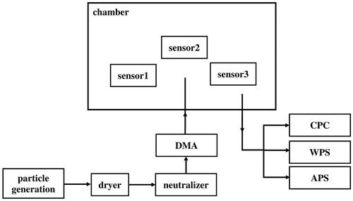
The DMA was operated to output particles with singly-charged equivalent diameter of 0.1, 0.3, 0.5, and 0.7 µm. The particles from the DMA include multiply-charged particles of the same mobility. The mobility-classified particles from the DMA were injected into the chamber and sampled by the sensors and the reference instruments. Data from the sensors and the different instruments were continuously collected using an external data acquisition system. Between tests with particles of different mobilities, the chamber was cleaned by passing clean air for at least 10 min to minimize background particle concentration.

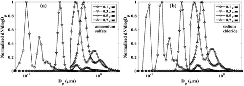
The size distributions of the different mobility-classified test particles, obtained using the combination of APS and WPS, are shown in Figure 2. As expected, several modes of multiply charged particles are generated for all the test particles. The maximum contribution of larger particles are seen when sodium chloride particles with singly-charged diameter of 0.1 µm are selected. As light scattering signatures have a strong dependence on particle size, the presence of even a small number of the larger multiply-charged particles must be considered in our data analysis. To improve data quality for inversion, we eliminated the contribution of small particles in the tail of the size distribution. This size distribution modification affected less than 10% of the total concentration and was done to minimize noise in the size distribution. The small particles have a relatively minimal contribution to the sensor light scattering signal but the noisy nature of the sampled particle size distribution complicates inversion.

Figure 2. Size distribution of particles used for sensor calibration. (a) Ammonium sulfate; (b) sodium chloride.

During the experiments, inside the chamber the temperature was in the range of 22 °C to 25 °C, and the RH varied in the range of 50% to 70%. The particle number concentration ranged from ∼50 to 6000 cm⁻³.

4. Results

4.1. Time series

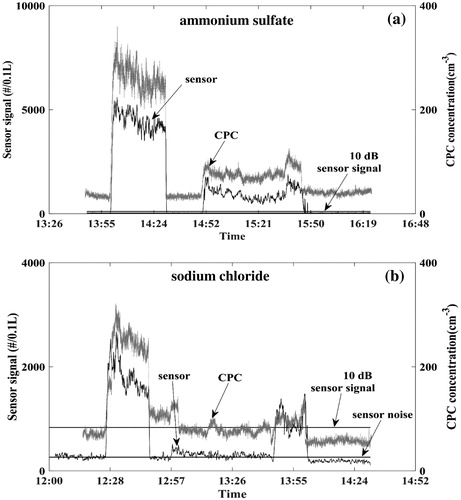
Time series data of total particle number concentration measurements from one of the tested Plantower sensors (i.e., Channel >0.3 µm) and the CPC are shown in Figure 3 for 0.5 and 0.7 µm testing particles. The signals are largely coincident with each other. When the chamber is cleaned, i.e., between the chamber tests, the particle number concentration is typically <100 cm⁻³. The combination of sensor noise and background signal are labeled as noise in the figures. The sensor noise is mainly contributed by the electrical and thermal properties of the sensor components, and the background signal is the response of particles detected by the CPC. To control data quality for sensor transfer function analysis, the data are screened based on the 10 dB signal criteria (i.e., signal below ∼3.2 times of the noise is removed for further analysis). For the two types of particles tested on different days, the background particle concentration levels are different. Based on the data filtration criteria listed above, almost the entire ammonium sulfate data are good for analysis while some of the data obtained with sodium chloride had to be eliminated.

Figure 3. Time series of Plantower sensor number concentration signal at the channel >0.3 µm when 0.5 and 0.7 µm particles are tested: (a) ammonium sulfate; (b) sodium chloride.

4.2. Transfer function

Applying the 10 dB screened sensor signal and following the method detailed in Section 2, the transfer functions for the different sensor channels are obtained using two types of test particles [NaCl and (NH₄)₂SO₄] used in our experiments. Using the DMA generated (NH₄)₂SO₄ particles of varying sizes (0.1, 0.3, 0.5, and 0.7 µm), the calculated sensor transfer function for the first particle number concentration channel (>0.3 µm) is shown in Figure 4. Tests with different sized particles allow for transfer function calculation over different size range. Combining results from all the test particles, transfer functions were obtained over a broad size range.

Figure 4. Calculated sensor transfer function at channel >0.3 µm using the method described in Section 2. The experimental data of ammonium sulfate particles of sizes 0.1, 0.3, 0.5, and 0.7 µm are used for the calculation.

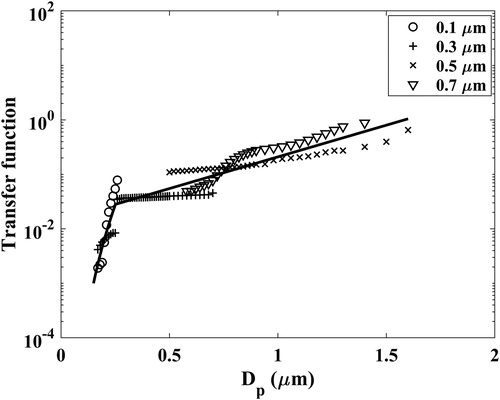
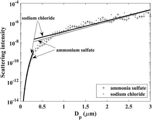
The spread in the transfer function values calculated with the different DMA-classified particles reflects the uncertainty in the inversion results. A single final sensor transfer function for a selected channel is established with a regression fit to the calculated transfer functions. For simplicity, a log-log linear fit (log(signal) vs log(particle diameter)) is used to represent the transfer functions for a size range of <∼0.3 µm and a log-linear [log(signal) vs particle diameter] fit is used for a size range of >∼0.3 µm. The choice of these fitting functions is consistent with the shape of the single particle light scattering curves which is illustrated in Figure 5. The dimensionless Mie scattering intensities corresponding to the illumination and detection geometry parameters of the Plantower sensor (scattering angle of 90^° and light wavelength of ∼0.65 µm) for ammonium sulfate and sodium chloride particles are calculated as a function of particle size (Mätzler 2002). Using the same form of the fitting equation for the two size ranges, as in Figure 4, the scattering curves of particles of the two compositions can be reasonably captured. As the Plantower sensor operates on the principle of light-scattering for particle number measurements, it is not surprising that the shape of the transfer function matches that of the Mie scattering curve.

Figure 5. Light scattering curve with particle size. The markers are the corresponding values calculated from the Mie scattering theory, and the curves are the fitted ones.

The transfer function calculation and fit function analysis is then extended to all 6 size channels of number concentration measurement. Considering that the Mie scattering curve is only dependent on particle effective refractive index for given wavelength and scattering angle, it is reasonable to assume that the same slope can be used to describe the transfer functions of all 6 size channels for a specific particle type. This assumption is confirmed with the fits for the transfer function for the different channels as shown in Figure 6. Unlike the number concentration transfer functions, for the mass concentration (PM) channels, it is seen that a second order curve is required to fit the log-linear transfer function. The transfer functions of all 3 PM channels can be fit with lines of the same slope, as shown in Figures 6h–i.

Figure 6. Sensor transfer function calculated from Tikhonov regularization (the markers) and the curve fitting (the lines) in the two size ranges (<0.3 µm and >0.3 µm) for the channel: (a) >0.3 µm; (b) >0.5 µm; (c) >1.0 µm; (d) >2.5 µm; (e) >5.0 µm; (f) >10 µm; (g) PM1; (h) PM2.5; (i) PM10.

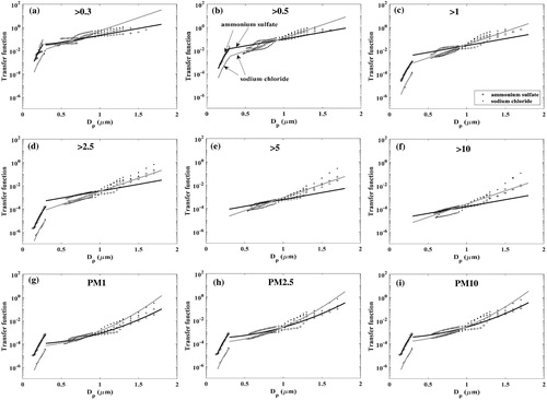
The sensor signal is seen to drop dramatically for particle diameters smaller than 0.3 µm, consistent with the lower detection size reported in the Plantower manual. The low sensitivity of the sensor in this size range (<0.3 µm) results in small, noisy signals that translate to significant uncertainty in our calculated signal response. Additionally, uncertainty in the test particle size distribution further adds to the calculated transfer function uncertainty in this size range.

As the slope of the curve fit are same for the different channels, the intercept of the curves distinguishes the channel transfer functions. The values of the transfer function slopes and intercepts, obtained with a fit over a size range of ∼0.1 µm to 1.7 µm, are listed in Table 1. We expect the slope of the transfer functions to vary with particle composition while the intercept will be dependent on both the composition and the channel size range. Additional tests using particles of different compositions is required to establish a relation between the transfer function parameters and particle properties.

Table 1. Parameters for the sensor transfer function curve fit shown in Figure 6.

Ammonium sulfate particles

Test particle size range

<0.3 µm

>0.3 µm

Sensor channel

>0.3

>0.5

>1

>2.5

>5

>10

PM1

PM2.5

PM10

>0.3

>0.5

>1

>2.5

>5

>10

PM1

PM2.5

PM10

slope

7.05

5.72

1.74

0.92

intercept

2.74

2.06

1.12

−0.11

–

–

−0.19

−0.17

−0.14

−2.20

−2.68

−3.33

−4.18

−4.83

−5.48

−3.87

−3.70

−3.44

Sodium chloride particles

Test particle size range

<0.3 µm

>0.3 µm

Sensor channel

>0.3

>0.5

>1

>2.5

>5

>10

PM1

PM2.5

PM10

>0.3

>0.5

>1

>2.5

>5

>10

PM1

PM2.5

PM10

slope

6.66

5.95

2.65

1.39

intercept

1.49

0.80

−0.13

−1.36

–

–

−1.35

−1.33

−1.30

−2.99

−3.47

−4.12

−4.97

−5.62

−6.27

−4.26

−4.09

−3.82

5. Validation and application

The sensor transfer function is obtained from the calibration experiments using monodispersed particles. For independent validation, the sensors were challenged with polydispersed particles generated by nebulizing 2.5% ammonium sulfate solution using the similar setup shown in Figure 1 without a DMA. Three Plantower PMS5003 sensors, different from those used during the calibration experiment, were used for this validation test. The tests were conducted with total particle number concentrations ranging from 3e4 and 5e4 cm⁻³.

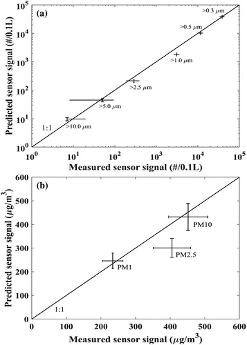
Particle size distributions were repeatedly measured five times using the reference instrument (WPS). The sensor signals were then predicted considering the obtained transfer function in Section 4 and the particle size distributions measured by the WPS instrument. The predicted and measured sensor signals for all the 9 channels are shown in Figures 7 (number concentrations in Figure 7a and PM in Figure 7b). Also shown in the figure is a comparison between the measurement and the prediction for the different channels. The predicted sensor signal closely matches measured values for most channels. The greatest deviations are observed for the >1.0 µm number concentration channel and PM2.5 values. For both the >1.0 µm number concentration and PM2.5 channel, the predictions are slightly lower than the measurements.

Figure 7. Comparison between the measured sensor signal and the prediction from the transfer function developed in this study (a) particle number concentration for the six size channels; (b) three particle mass concentrations. The uncertainty in measured signal value is determined using error propagation of the maximum deviation from the average value of the three sensors during the entire experimental validation period. The uncertainty in predicted values is defined as the standard deviation of total particle number concentration measured by the CPC during the validation period.

Note that, previous studies have shown that RH can affect measurements of some optical-based low-cost sensors (e.g., Jayaratne et al. 2018). In our experiments, calibration was conducted with dry particles and with air humidity in the chamber at 50%–70% RH, while the air humidity in the validation experiment was <10% RH. Even though the two humidities are quite different, the nature of the test particles is likely the same as these particles should not experience any deliquescence in the chamber when RH < 70% (Vlasenko et al. 2017).

The sensor transfer functions can be used to understand the theoretical sensor response under different particle test conditions. We examine the sensor response under two scenarios – ideally single size of ammonium sulfate particle: 0.2 and 1.0 µm. From the results shown in Figure 8, the following observations are made:

Figure 8. Predicted sensor signal for ammonium sulfate particles based on the transfer function fitting curves in Table 1. (a) Size distribution signal from 1000 cm⁻³ 0.2 µm particles; (b) size distribution signal from 10 cm⁻³ 1.0 µm particles; (c) PM signal from 1000 cm⁻³ 0.2 µm particles; (d) PM signal from 10 cm⁻³ 1.0 µm particles. The dashed lines at (c) and (d) are calculated mass concentrations based on spherical particle assumption.

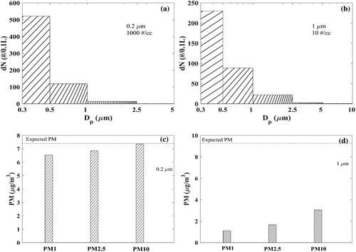
1. Even when the sensors are exposed to particles smaller than the listed lowest detection size (0.3 µm), a finite sensor signal response will be observed in all channels, as shown for 0.2 µm monodisperse particles in Figure 8a.

2. The Plantower sensor signals always show a monotonically decreasing particle size distribution with increasing diameter channel, regardless of the actual particle size distribution. As shown in Figure 8b, even for 1.0 µm monodisperse particles, the strongest signal is detected in the first channel rather than at the channel corresponding to the test particle size.

3. The mass concentrations (PM) are under-estimated by the sensor for both particle sizes, as shown in Figures 8c and d. The under-estimation is seen to be greater when the particles are larger in size. Based on the transfer functions, the Plantower sensor responds more like a nephelometer than a single particle scattering spectrometer. Our predictions of underestimation of PM by Plantower is consistent with that expected from nephelometers (Tryner et al. 2019).

The example in Figure 8 demonstrates the importance of a calibration model for a low-cost sensor in great detail. As the sensor response strongly depends on the particle size distribution and refractive index, any changes in ambient particle properties will affect sensor accuracy. Using the physical property based calibration model, a relatively accurate particle size distribution could potentially be retrieved from the low-cost sensor signal. Additionally, if particle size distribution is known, it might be possible to obtain other particle information, such as effective refractive index, using knowledge of the sensor transfer function.

6. Conclusion

The use of low-cost sensors for ambient monitoring requires knowledge of the sensor performance characteristics. A critical element of sensor performance is its size-dependent detection efficiency or transfer function. Here, we make the first ever determination of transfer function of a popular low-cost sensor, Plantower PMS5003, using particles of two compositions (ammonium sulfate and sodium chloride) generated using a DMA. To calculate the transfer function, we first describe the signal equation of the sensor. The signal is then inverted using Tikhonov regularization to calculate the sensor transfer functions. Experiments conducted with mono-mobility particles corresponding to singly-charged 0.1, 0.3, 0.5, and 0.7 µm particles provide a rich data set for transfer function calculation. Using a quadratic programing method with the constraints of monotonic increase with particle size and non-negativity, the sensor transfer function is calculated for the 9 channels of the Plantower sensor. Our results show that the transfer function curves for the number concentration channels have similar characteristics as the Mie scattering curve.

The calculated transfer functions are then validated with an independent experiment using polydispersed particles. The calculated signals in the different channels are seen to match measured values with reasonable accuracy, which indicates that the physical-property based transfer function can be useful for calibration of a low-cost aerosol sensor. Using the transfer function to examine the sensor response for two different monodispersed particles, it is seen that (1) the as-reported particle number distributions from the 6 channels of the sensor may not reflect actual size distributions and can be significantly erroneous; (2) the reported PM values may be an under-estimate, especially for larger sized particles. This first study on the transfer functions of the Plantower PMS5003 sensor provides us with a critical theoretical basis to understand and improve the accuracy of the sensor response when operated under different ambient conditions.

Additional information

Funding

We would like to thank the funding support for this project from the New York State Energy Research and Development Authority (NYSERDA, Grant No. 119410).

References

- Bulot, F. M. J., S. J. Johnston, P. J. Basford, N. H. C. Easton, M. Apetroaie-Cristea, G. L. Foster, A. K. R. Morris, S. J. Cox, and M. Loxham. 2019. Long-term field comparison of multiple low-cost particulate matter sensors in an outdoor urban environment. Sci. Rep. 9 (1):7497. doi: 10.1038/s41598-019-43716-3.
- Dubey, P., and S. Dhaniyala. 2013. Improved inversion of scanning electrical mobility spectrometer data using a new multiscale expectation maximization algorithm. Aerosol. Sci. Technol. 47 (1):69–80. doi: 10.1080/02786826.2012.728014.
- Garda, B., and Z. Galias. 2014. Tikhonov regularization and constrained quadratic programming for magnetic coil design problems. Int. J. Appl. Math. Comput. Sci. 24 (2):249–57. doi: 10.2478/amcs-2014-0018.
- Hansen, P. C. 2008. Regularization tools: A matlab package for analysis and solution of discrete ill-posed problems. Version 4.1 for Matlab 7.3. Informatics and Mathematical Modelling. Technical University of Denmark, Lyngby, Denmark. doi: 10.1007/BF02149761.
- He, M., and S. Dhaniyala. 2012. Vertical and horizontal concentration distributions of ultrafine particles near a highway. Atmos. Environ. 46:225–36. doi: 10.1016/j.atmosenv.2011.09.076.
- Jayaratne, R., X. Liu, P. Thai, M. Dunbabin, and L. Morawska. 2018. The influence of humidity on the performance of a low-cost air particle mass sensor and the effect of atmospheric fog. Atmos. Meas. Tech. 11 (8):4883–90. doi: 10.5194/amt-11-4883-2018.
- Kelly, K. E., J. Whitaker, A. Petty, C. Widmer, A. Dybwad, D. Sleeth, R. Martin, and A. Butterfield. 2017. Ambient and laboratory evaluation of a low-cost particulate matter sensor. Environ. Pollut. 221:491–500. doi: 10.1016/j.envpol.2016.12.039.
- Knutson, E. O., and K. T. Whitby. 1975. Aerosol classification by electric mobility: Apparatus, theory, and applications. J. Aerosol Sci. 6 (6):443–51. doi: 10.1016/0021-8502(75)90060-9.
- Lazer, D., R. Kennedy, G. King, and A. Vespignani. 2014. Big data. The parable of Google Flu: Traps in big data analysis. Science 343 (6176):1203–5. doi: 10.1126/science.1248506.
- Malings, C., R. Tanzer, A. Hauryliuk, P. K. Saha, A. L. Robinson, A. A. Presto, and R. Subramanian. 2019. Fine particle mass monitoring with low-cost sensors: Corrections and long-term performance evaluation. Aerosol Sci. Technol.:1–40. doi: 10.1080/02786826.2019.1623863.
- Mätzler, C. 2002. Matlab functions for Mie scattering and absorption. Research Report No. 2002-08, University of Bern, Institute of Applied Physics, Bern.
- Snyder, E. G., T. H. Watkins, P. A. Solomon, E. D. Thoma, R. W. Williamas, G. S. W. Hagler, D. Shelow, D. A. Hindin, V. J. Kilaru, and P. W. Preuss. 2013. The changing paradigm of air pollution monitoring. Environ. Sci. Technol. 47 (20):11369–77. doi: 10.1021/es4022602.
- Tikhonov, A., and V. Arsenin. 1977. Solutions of ill-posed problems. Washington, DC: John Wiley & Sons.
- Tryner, J., N. Good, A. Wilson, M. L. Clark, J. L. Peel, and J. Volckens. 2019. Variation in gravimetric correction factors for nephelometer-derived estimates of personal exposure to PM2.5. Environ. Pollut. 250:251–61. doi: 10.1016/j.envpol.2019.03.121.
- Vlasenko, S. S., H. Su, U. Pöschl, M. O. Andreae, and E. F. Mikhailov. 2017. Tandem configuration of differential mobility and centrifugal particle mass analysers for investigating aerosol hygroscopic properties. Atmos. Meas. Tech. 10 (3):1269–80. doi: 10.5194/amt-10-1269-2017.
- Wang, Y., and C. Yang. 2008. Regularizing active set method for retrieval of the atmospheric aerosol particle size distribution function. J. Opt. Soc. Am. A 25 (2):348–56. doi: 10.1364/JOSAA.25.000348.
- Wolfenbarger, J. K., and J. H. Seinfeld. 1990. Inversion of aerosol size distribution data. J. Aerosol. Sci. 21 (2):227–47. doi: 10.1016/0021-8502(90)90007-K.
- Zimmerman, N., A. A. Presto, S. P. N. Kumar, J. Gu, A. Hauryliuk, E. S. Robinson, and A. L. Robinson, and R. Subramanian. 2018. A machine learning calibration model using random forests to improve sensor performance for lower-cost air quality monitoring. Atmos. Meas. Tech. 11 (1):291–313. doi: 10.5194/amt-11-291-2018.