Evaluation of low-cost optical particle counters for monitoring individual indoor aerosol sources

Abstract

Low-cost optical particle counters (OPC) have gained increasing attention in recent years in exposure studies. Previous studies reported that the OPCs’ performance varies considerably with type of particles being measured; however, little information on their performance in monitoring common indoor aerosols is available. Given the significance of exposure to indoor aerosols and their associated adverse health effects, this experimental study investigates the performance of low-cost OPCs in monitoring individual aerosols that are commonly found indoors in a controlled chamber environment. Performances of four low-cost OPCs were examined under exposure to varying concentrations of biological (dust mite, pollen, cat, and dog fur) and non-biological (monodisperse silica and melamine resin) aerosols. Each particle sample was dispersed into the chamber using a computer-controlled syringe injection system, while size-resolved particle number concentrations were simultaneously measured by four low-cost OPCs (OPC N2, IC Sentinel, Speck, and Dylos) as well as a lab-grade reference sensor (AeroTrak). The study results showed measurable effects of particle size, particle type, and concentration on the low-cost OPC responses. Particle concentration had the most dominant effect on the linearity of low-cost sensors. Results also revealed that the sensor responses to four biological particles follow a similar pattern and converge to a linear line as the number concentration increases above 5 cm⁻³. As for non-biological particles, the OPC responses were more varied depending on the particle type and size, especially in the concentration range <10 cm⁻³. Calibration equations developed in this study provide baseline information for correcting low-cost OPC readings when utilized to measure concentrations of individual indoor aerosol sources.

Copyright © 2019 American Association for Aerosol Research

EDITOR:

• Kihong Park

1. Introduction

Human exposure to airborne particulate matter (PM) is detrimental to human health and well-being (Pope III et al. 2002; Danesh Yazdi et al. 2019). High cost of PM sensors has been a barrier to the long-term PM monitoring with sufficient spatial and temporal resolution (Castell et al. 2017). However, recent emergence of low-cost PM sensor technology has enabled real-time PM monitoring with high spatiotemporal resolution in both indoor and outdoor environments (Rai et al. 2017). Such capabilities have opened new horizons in the exposure science for various applications such as 1) integrating PM sensors into building systems to control occupant exposure to indoor PM (Kumar, Martani, et al. 2016; Kumar, Skouloudis, et al. 2016); 2) establishing outdoor PM monitoring networks with high spatiotemporal resolutions (Jiao et al. 2016); and 3) increasing public awareness about air pollution through projects such as Citizen Science (Bandini, Mosca, and Palmonari 2007; Jovašević-Stojanović et al. 2015).

Many of low-cost PM sensors in the market are light-scattering based optical particle counters (OPCs). In most OPCs, a pump-driven sheath airflow directs the sampled particles into the sensing region that is illuminated by a focused light beam. The light source is usually broadband (white light) or monochromatic (laser or LED). As the sampled particles pass through the sensing region, they scatter light at different rates depending on their size, shape, and the light wavelength (Bohren and Huffman 2004). The amount of light scattering is detected over a specific range of angles and translated to an electronic pulse (Horvath 2009). The electronic pulse height is then converted to particle size using Mie theory so that size-resolved particle number counts are measured by an OPC (Kulkarni, Baron, and Willeke 2011; Hinds 2012).

Although many low-cost OPCs overall have a similar working principle, they vary with light source wavelength, light scattering detection angle, and number of particle size bins. Also, while most OPCs use a pump to sample ambient air and send it to the sensing region, some sensors utilize passive sampling methods such as natural convection (Weekly et al. 2013). To address the necessity of independent scientific investigation of low-cost sensor performance, several researchers have conducted field and laboratory studies of observational and experimental nature (see Table S1 in the online supplementary information [SI] for a summary of the studies on low-cost sensors tested in this study). Sousan et al. (2016) tested Dylos1700 (Dylos, Riverside, CA) sensor in a chamber with salt, Arizona road dust (ARD), welding fume, and diesel exhaust particles. Their results showed that particle detection efficiency ranged from 0.04% to 108% for particle sizes of 0.1 to 5 µm. The linear calibration slope for linear response region varied dramatically with particle type (i.e., 2.6 for salt particles and 54 for diesel fume particles). Similar influence of particle type on the PM sensor performance was found by Manikonda et al. (2016) while testing Dylos1700, Dylos1100 pro (Dylos, Riverside, CA), and Speck (Airviz Inc., Pittsburgh, PA) sensors in a chamber emission study with cigarette smoke and Arizona Test Dust (ATD). In another laboratory chamber study by Wang et al. (2015), three low cost PM sensors (PPD42NS-Shinyei, DSM501A-Samyoung, and GP2Y1010AU0F-Sharp) were tested by comparing the sensor responses to NaCl particles, sucrose, NH₄NO₃ particles, and atomized PSL particles sized in 300, 600, 900 nm. Besides lab experiments, field co-location campaigns were conducted and revealed the influence of surrounding microenvironment on the performance of low-cost particle sensors (Patel et al. 2017; Steinle et al. 2015; Gao, Cao, and Seto 2015; Kelly et al. 2017; Mukherjee et al. 2017; Zikova, Hopke, and Ferro 2017). Another study (Snyder et al. 2013) also warned of detrimental consequences of rushing to apply low-cost sensors to a specific field measurement without proper performance evaluation and quality control. One major concern of using low-cost PM sensor networks has been the quality of the collected data and long-term calibration drift. In order to mitigate this issue, recently, machine learning and data fusion algorithms are being used (Zimmerman et al. 2017; Castell et al. 2018). Taken together, controlled laboratory and field studies have shown that particle type, size, and concentrations being measured are major influencing factors for the performance of low-cost OPCs.

However, very little information is available about the performance of low-cost PM sensors in detecting indoor aerosols. Especially, none of the controlled laboratory studies have examined performance of low-cost PM sensors in measuring common indoor biological aerosols. Given this background, the objective of the present study is to evaluate the performance of low-cost PM sensors in monitoring individual aerosols that are commonly found indoors while varying particle type, size, and concentration, and to examine how the sensor responses differ between biological and non-biological aerosols.

2. Materials and methods

Four low-cost PM sensors were tested in a controlled environmental chamber while varying particle type, size, and concentration level. The following sections describe details of data collection (Section 2.1), sensors characteristics (Section 2.2), tested biological and non-biological particle characteristics (Section 2.3), and data analysis method (Section 2.4).

2.1. Test chamber set-up and experimental protocol

Figure 1 illustrates the laboratory experimental set-up. A 0.76 × 0.76 × 0.42 m particle dispersion chamber was used to test the low-cost PM sensors in a controlled environment. In order to test the sensors under exposure to varied particle concentrations, the experiment was designed in a particle-decay fashion. For the particle decay test, a pulse injection of particles into the chamber was performed. The particle injection was made by using a syringe, as it was easily detached, cleaned, and replaced for multiple tests. A computer-controlled system was designed to inject the particles into the chamber. The particle injection system dispersed the particles inside the chamber by colliding two airflow jets (a particle-laden air jet and a particle-free air jet) in the middle of the chamber. As shown in Figure 1, the particle-laden air jet was delivered from the bottom center inlet that was supplied by Line 1, while the particle-free air jet was from the top center inlet supplied by Line 2. The particle-free airflow was directly supplied to the chamber after passing a HEPA filter (TSI Inc., Shoreview, MN); however, particle-laden airflow in Line 1 involved another step to add test particles to the HEPA-filtered airflow before supplying it to the chamber. A syringe was used to add the desired amount of test particles into the airflow (see Figure 1).

Figure 1. Schematic of the chamber experiment set-up.

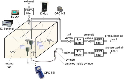
A combination of the solenoid and ball valves were used to control the airflow in each of the two pressurized airflow lines. Solenoid valves, which were controlled by a computer program, were used to open and close the airflow lines while ball valves were used to modulate the airflow rate passing through each line. The ball valves were used to set a specific airflow rate before the test was started. To ensure the accuracy and consistency of airflow rates throughout different tests, a flow meter was used to measure the airflow rate in each line. After setting the position of the ball valve before the test, it was not changed anymore during the test. To control the airflow rate between 0% and 100% of the desired airflow rate, which was set by the ball valve, solenoid valves were used. In order to prevent infiltration of aerosols, the chamber was over-pressurized during the experiment. A port connected to a one-way valve and a HEPA filter was used to create a dedicated filtered exhaust path for the over-pressurized chamber airflow and avoid exfiltration of test particles into the lab environment. The exhaust port (shown in Figure 1) was located at the top back left corner of the chamber.

Four mixing fans were running at the four corners of the chamber to enhance a well-mixed condition in the chamber. However, since the well-mixed condition is not always achieved perfectly, we designed the chamber, particle injection, and sampling in a way that, even in the event of the well-mixed condition not being met, sensors could sample similar particle distribution and concentration. The tested sensors were placed inside the chamber such that they have a similar radial distance from the particle injection inlet - at the center of the chamber - and also at a similar height from the chamber floor. Besides using the mixing fans to improve the aerosol mixing in the chamber environment, the sensor location arrangement allows for homogeneous aerosol sampling by the sensors.

Nine 2.5-h particle-decay test cases were conducted. Each test was performed using the following six steps:

1. Before each test, all chamber surfaces as well as the particle injection line were thoroughly cleaned and washed to remove any residual particles from previous tests.

2. The specific amount of test particles needed to create the desired maximum particle number concentration in the chamber was calculated, measured, and added to the syringe.

3. The intent of setting a maximum particle number concentration was mainly not to exceed the detection limit of the reference device. Most of the tested particles were polydisperse, therefore for calculating the particle mass for injection, the geometric mean particle size and density were used. It should be noted that the calculated amount of mass for injection was not meant to be an exact representation of number concentration of any specific size fraction, but rather an estimate of total number concentration that does not go beyond the maximum limit of the reference device. Note that as each experiment was designed as a particle concentration decay test, the sensors were exposed to a range of concentrations from the maximum and all the way down to the background level.

4. Particle-free air at a volumetric flow rate of 9 L/min was supplied to the chamber for at least 30 min to flush the chamber until the reference PM sensors report PM counts of close to zero. Four mixing fans were running at the four corners of the chamber to achieve a well-mixed condition.

5. Background PM monitoring was performed by all sensors for initial 5 min (minutes 0 to 5 of the test).

6. A signal was sent to the solenoid valve in Line 1 to supply 18 L/min of filtered air flow to the syringe and inject the particles into the chamber for 2 min (minutes 5 to 7 of the test).

7. The solenoid valve in Line 1 was closed and the particles decay started. Size-resolved particle concentrations were monitored until it reached the background levels (minutes 7 to 150 of the test).

2.2. Sensor specifications

The present study examined performance of four different low-cost PM sensors: 1) OPC N2 (Alphasense Ltd., Essex, UK), 2) IC Sentinel (Oberon Inc., State College, PA, USA), 3) Speck (Airviz Inc., Pittsburgh, PA, USA), and 4) Dylos (Dylos, Riverside, CA, USA). Figure S1 in the SI shows four low-cost sensors and the reference sensor examined in this study. All tested low-cost sensors are optical-based particle counters that measure the particle number concentrations. AeroTrak (TSI 9306, TSI, Inc., Shoreview, MN, USA) was used as the reference monitor, given that it is a lab-grade optical particle counter and can measure particle number concentrations in the 0.3–14 µm diameter range with six particle size bins (0.3–0.5 µm, 0.5–1.0 µm, 1.0–2.5 µm, 2.5–5 µm, 5–10 µm, and >10 µm). The counting efficiency of AeroTrak is 50% at 0.3 µm and 100% for particles >0.45 µm. Manufacturer calibration was performed for our tests and the size-resolved uncertainty of AeroTrak ranged from 3.6 to 4.1% for the particle size range of 0.3–10 µm (see Table S2 in the SI). Table 1 summarizes the detailed light source and flow characteristics and of the tested low-cost sensors.

Table 1. Summary of the tested particle sensor characteristics.

Low-cost and reference sensors	Particle detection technology	Light source wavelength (nm)	Detection size range (µm)	# of bins	Bin size cuts (µm)	Flow rate (L/min)	Measurement time resolution (s)	Concentration detection limit
OPC N2 (Alphasense)	Laser diode	658^2	0.38–17	16	0.46, 0.66, 0.92, 1.20, 1.47, 1.83, 2.54, 3.50, 4.50, 5.75, 7.25, 9.00, 11.00, 13.00, 15.00, 16.75	Sampling: 0.22, total:1.2	1	3.40 × 10^11 particles/m^3
IC Sentinel	Laser diode, 10 mW	650^3	0.5-NR^6	4	0.5, 1, 5, 10	1.5	120	1.32 × 10^11 particles/m^3
Speck^1	LED	850^4	0.5–3	1	2	NR^6	30	NR^6
Dylos (DC1100)	NR^6	650	>1	2	1,5	0.283	60	NR^6
AeroTrak (TSI 9306)	Enhanced active cavity HeNe laser	785^5	0.3–14	6	0.3, 0.5, 1.0, 3.0, 5.0, 10.0	2.83	1	1.40 × 10^11 particles/m^3 at 5% coincidence loss

1: Uses DSM501A (Syhitech DSM501, Syhitech Co., Ltd) sensor.

2: Laser diode.

3: Laser diode, 10 mW.

4: LED.

5: Enhanced active cavity HeNe laser.

6: Not reported.

2.3. Tested particles characteristics

The low-cost PM sensors were tested with nine different dry powder particle batches. Table 2 summarizes the detailed characteristics of the tested particles. These batches included biological and non-biological as well as monodisperse and polydisperse particles. Four types of biological particles commonly found in indoor environments (Bardana Jr 2001) were used to test the PM sensors; 1) dust mite (Indoor Biotechnologies Inc., Charlottesville, VA, USA), 2) pollen (GREER, Lenoir, NC, USA), 3) cat fur, 4) and dog fur. Detailed descriptions of preparing cat fur and dog fur dust particles are provided in a previous study (Salimifard et al. 2015, 2017). Besides the four types of biological particles, the tests included four batches of monodisperse non-biological particles (microparticles Gmbh, Berlin, Germany): 1) melamine resin (MF-R) in 1.041 µm, 2) melamine resin (MF-R) in 2.81 µm, 3) silicon dioxide (SiO₂-R) in 0.977 µm, 4) silicon dioxide (SiO₂-R) in 2.81 µm. In addition, polydisperse quartz particles (crushed quartz #10 bt # 4339, Particle Technology Limited, UK) were tested. Figure 2 shows size distributions of the polydisperse biological and quartz particles.

Figure 2. Particle size distribution of tested polydisperse particles during the first minute of particle injection measured by the reference sensor (AeroTrak, TSI): (a) dust mite, (b) pollen, (c) cat fur, (d) dog fur, and (e) quartz.

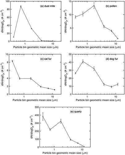
Table 2. Summary of the tested particles.

Particle type	Size distribution type	Size range (µm)	Biological/ non-Biological	Density (kg/m^3)	Shape	Roughness	Refractive index
Dust mite	Polydisperse	0.58–48^a	Biological	1140^a	Rounded**^,b	Smooth	–
Pollen	Polydisperse	–	Biological	850^b	Near spherical^b	–	1.5^c
Cat fur	Polydisperse	0.58–409^a	Biological	1000^a	Fibers^a	Rough	1.35–1.43^d
Dog fur	Polydisperse	0.58–35^a	Biological	1000^a	Fibers^a	Rough	1.37–1.55^d
Melamine resin (MF-R)	Monodisperse	1.041 ± 0.03*, 2.81 ± 0.06*	Non-biological	1510^e	Spherical^e	Smooth^e	1.68^e
Silicon dioxide (SiO2-R)	Monodisperse	0.977 ± 0.026*, 2.81 ± 0.1*	Non-biological	1850^e	Spherical^e	Smooth^e	1.5^f
Crushed quartz (>95% of SiO2)	Polydisperse	0.58–22.5^a	Non-biological	2650^a	Varied***^,a	Smooth	1.544^b

* Size ± standard deviation.

** With prismatic edges resulted from the ball mill crushing effect).

*** Varied from squares to rectangles (5/1 ratios maximum).

^aParticle size distribution is shown in Figure 2 and density information is based on a previous study (Salimifard et al. 2017).

^bHinds (2012).

^cGullvåg (1964).

^dYan et al. (2015).

^eAs provided by the manufacturer.

^fRadhakrishnan (1947).

2.4. Data analysis

In analyzing the performance of the low-cost sensors, particles smaller than 2.5 µm are particularly the focus of this study. The main reason for selection of this size range is that the size range representing PM_2.5 is the only size range that all tested sensors in this study have in common. Moreover, PM_2.5 is the size range that most other available low-cost sensors cover (Rai et al. 2017; Jovašević-Stojanović et al. 2015) and also the focus of many other particle sensing studies (Kelly et al. 2017; Gao, Cao, and Seto 2015; Zikova, Hopke, and Ferro 2017; Johnson et al. 2018; Holstius et al. 2014; Steinle et al. 2015; Yanosky, Williams, and MacIntosh 2002). As particle size detection range varies with sensor, size bins representing the particle smaller than 2.5 µm that had the closest overlap with other sensors were selected for each sensor. For instance, Speck sensor covers a particle size bin of 0.5–3 µm, while AeroTrak measures particles in a size range of 0.3–3 µm. Note that the contribution of particles >2.5 µm to total number concentration is marginal (see Figure 2). Table 3 summarize information about particle size detection range for each sensor.

Table 3. Tested sensors’ size bins representing particles smaller than 2.5 µm.

Low-cost and reference sensors	Size detection range (µm)
OPC N2 (Alphasense)	0.38–3
IC Sentinel	0.5–5
Speck	0.5–3
Dylos (DC1100)	1–5
AeroTrak (TSI 9306)	0.3–3

The low-cost sensors tested in this study had different time resolutions ranging from 1 s to 2 min. In order to compare sensor readings against each other, all the recorded data were time-averaged in 2-min intervals. After synchronizing the monitoring time-interval for all sensors, the performance of low-cost sensors was examined using a regression analysis.

Linear regression coefficients provide straightforward indicators of a sensor performance compared to the reference instrument. If sensor readings perfectly match the reference instrument readings, the regression model exhibits an intercept of 0 and a slope of 1. If the intercept and slope coefficients are significantly different from 0 and 1, respectively, it suggests fixed and proportional systematic biases with respect to the reference sensor. The coefficient of determination (R²) measures the correlation between the test and reference sensors, while the root mean square error (RMSE) gauges the precision of the test sensor compared to the reference sensor (Yanosky, Williams, and MacIntosh 2002). Linear regression is commonly used in the literature for analyzing the performance of a sensor of interest (dependent variable) versus the reference sensor (independent variable). Among several regression models, Ordinary Least Squares (OLS) is the suitable and most commonly used model in sensor performance and calibration analysis (Holstius et al. 2014; Manikonda et al. 2016; Patel et al. 2017; Wang et al. 2015; Sousan et al. 2017).

Once the linear regression model (Equation (1)(1) $$y=\mathrm{FB}+\mathrm{PB}\times x$$(1) ) for a low-cost sensor is developed, a calibration equation (Equation (3)(3) $${\mathrm{NC}}_{\mathrm{LCS},\mathrm{corrected}}=-\frac{\mathrm{FB}}{\mathrm{PB}}+\left(\frac{1}{\mathrm{PB}}\right){\mathrm{NC}}_{\mathrm{LCS}}$$(3) ) can be calculated to address the fixed and proportional biases. (1) $$y=\mathrm{FB}+\mathrm{PB}\times x$$(1) (2) $$x=-\frac{\mathrm{FB}}{\mathrm{PB}}+\left(\frac{1}{\mathrm{PB}}\right)y$$(2) (3) $${\mathrm{NC}}_{\mathrm{LCS},\mathrm{corrected}}=-\frac{\mathrm{FB}}{\mathrm{PB}}+\left(\frac{1}{\mathrm{PB}}\right){\mathrm{NC}}_{\mathrm{LCS}}$$(3)

where,

• x (independent variable) is the number concentration measured by the reference sensor ($\#/{\mathrm{cm}}^3$),

• y (dependent variable) is the number concentration measurement of the low-cost sensor estimated by the linear regression model ($\#/\mathrm{c}{\mathrm{m}}^3$),

• FB is the fixed bias (intercept of the regression model) ($\#/{\mathrm{cm}}^3$),

• PB is the proportional bias (slope of the regression model),

• ${\mathrm{NC}}_{\mathrm{LCS}}$ is the number concentration measured by the low-cost sensor ($\#/{\mathrm{cm}}^3$), and

• ${\mathrm{NC}}_{\mathrm{LCS},\mathrm{corrected}}$ is the corrected low-cost sensor number concentration ($\#/{\mathrm{cm}}^3$).

In order to quantify the uncertainty of the estimated calibration curves, repetition measurements for three test particles (dust mite particles and non-biological monodisperse particles of silicon dioxide and melamine resin) were conducted (see Figure S2 in the SI). The variation in the regression slope of low-cost sensor responses versus the reference sensor for multiple repetition measurements was calculated as a measure of the experimental uncertainty.

3. Results and discussion

3.1. Temporal particle concentration measurement

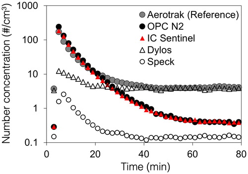
Figure 3 shows the concentration profiles of dust mite particles measured by the four low-cost sensors and the reference sensor over the background, emission, and decay periods. Note that tests with other types of particles exhibited similar trends. According to the experiment results, OPC N2 and IC Sentinel readings are fairly close to those of reference sensor when measuring higher concentration ranges (emission and early decay period); however, they underestimate concentrations in lower concentration ranges (background and late decay sampling periods). Speck and Dylos sensors consistently underestimate particle concentrations in higher concentrations, while their performance in lower concentration was varied during various tests. The discrepancies in the concentration profile and decay rate between the reference sensor and low-cost sensors reflect fixed and proportional biases for a given low-cost sensor. The following section provides details of such biases based on the regression analysis.

Figure 3. Time-series of dust mite particle number concentrations for the size range <2.5 µm measured by four low-cost sensors and the reference sensor. The test consists of three phases; 1) background level (minutes 0–5), 2) particle injection (minutes 5–7), and 3) particle concentration decay (minutes 7–150). Note that other test cases with different particle types and sizes had fairly similar temporal concentration profile trends.

3.2. Performance evaluation using regression analysis

The experiment results revealed that the performance of low-cost sensors is a strong function of particle concentration. Figure 4 shows comparison of the low-cost sensors with the reference sensor in measuring bioaerosol concentrations of 0–20 cm⁻³. All low-cost sensors, across different particle types being measured, showed a non-linear response in low concentrations in which as the sensor response became more linear as concentration increased. As shown in Figure 4, particle number concentration of 5 cm⁻³ is the concentration threshold that divides the non-linear response region (0–5 cm⁻³) and the linear response region (>5 cm⁻³) for biological particles. For the non-linear response region, the R² values are smaller than 0.645 for all four sensors regardless of the particle type. However, for the linear response region (>5 cm⁻³), the R² values are in the range of 0.708–0.999 for all sensors (see more details in Table 4). The clear contrast in R² values between the low and high concentration region reflects the effect of concentration on the linearity of low-cost sensor response.

Figure 4. Particle number concentrations measured by low-cost sensors (y-axis) versus the reference sensor (x-axis). Subplots in the left column (a, c, e, and g) represent the non-linear response region (0–5/cm³). Subplots in the right column (b, d, f, and h) represent the linear response region.

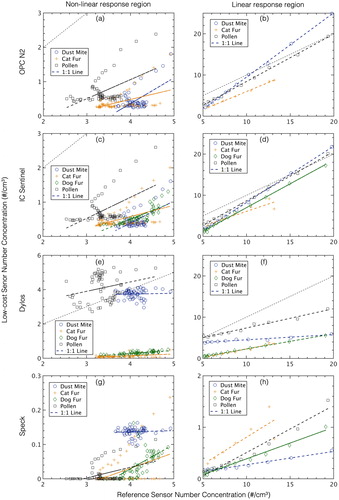
Table 4. Summary of regression analysis results for four tested bioaerosols comparing each low-cost sensor to the lab-grade sensor.

Particle type	Concentration range^a (#/cm^3)	OPC N2				IC Sentinel
		FB^b(#/cm^3)	PB^c	R^2	RMSE (#/cm^3)	FB (#/cm^3)	PB	R^2	RMSE (#/cm^3)
Dust mite	0–5	–2.64	0.751	0.320	0.250	–2.19	0.645	0.342	0.204
	5–20	–6.11	1.56	0.999	0.225	–5.39	1.37	0.999	0.194
Pollen	0–5	–1.17	0.556	0.248	0.350	–1.31	0.611	0.274	0.360
	5–20	–3.08	1.15	0.998	0.276	–3.30	1.20	0.998	0.255
Cat fur	0–5	–0.710	0.298	0.213	0.244	–0.740	0.330	0.213	0.272
	5–20	–2.77	0.875	0.997	0.146	–1.04	0.713	0.850	0.987
Dog fur	0–5	N/A				–1.53	0.508	0.645	0.131
	5–20					–4.53	1.15	0.997	0.278
Particle type		Speck				Dylos
	Concentration range^a (#/cm^3)	FB^b(#/cm^3)	PB^c	R^2	RMSE (#/cm^3)	FB (#/cm^3)	PB	R^2	RMSE (#/cm^3)
Dust mite	0–5	0.123	0.00343	0.00387	0.0125	3.55	0.0459	0.00163	0.259
	5–20	0.0158	0.0258	0.974	0.0214	3.24	0.128	0.918	0.192
Pollen	0–5	–0.0906	0.0310	0.161	0.0256	2.26	0.546	0.0645	0.752
	5–20	–0.404	0.0914	0.961	0.0915	2.71	0.467	0.977	0.360
Cat fur	0–5	–0.151	0.0454	0.176	0.0421	–0.242	0.0975	0.200	0.084
	5–20	–0.244	0.105	0.708	0.223	–1.89	0.418	0.957	0.291
Dog fur	0–5	–0.259	0.0718	0.402	0.0305	–0.443	0.180	0.523	0.0599
	5–20	–0.225	0.0613	0.983	0.0348	–1.39	0.369	0.998	0.0634

^aAs measured by the reference sensor.

^bFixed bias, intercept of regression model.

^cProportional bias, slope of regression model.

The results for each particle type are developed from one test.

Figures 4b, d, f, and h show the response of the low-cost sensors to each type of tested bioaerosols in the linear response region. In the linear response region, variations of the regression slopes (proportional bias) are distinctly smaller for OPC N2 and IC Sentinel (Figures 4b and d, respectively) compared to Dylos and Speck (Figures 4f and h, respectively). Note that the regression slopes for OPC N2 and IC Sentinel are fairly close to 1. However, Speck and Dylos sensors exhibit regression slopes much smaller than 1 with relatively large variations depending on the particle type.

As shown in Figure 4, the linear response concentration region chosen for the linear regression is 5–20 cm⁻³. This concentration region was selected, for it was the concentration region within which all the tested low-cost sensors demonstrated a linear response to the tested bioaerosols. For concentrations higher than 20 cm⁻³, while IC Sentinel and OPC N2 continued to demonstrate a linear response, Dylos and Speck exhibited a positive curvilinear relationship with respect to increased particle concentration until it reached the saturation point, followed by a negative curvilinear relationship (details shown in Figure 5).

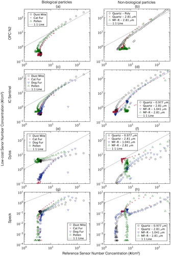
Figure 5. The response of low-cost sensors under exposure to biological (a, c, e, and g) and non-biological (b, d, f, and h) aerosols with respect to the reference sensor.

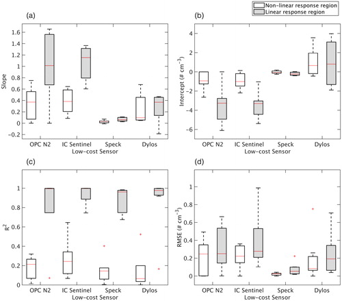
Figures 6a–c illustrate variations of regression slopes (PB), intercepts (FB), and values of R² for the linear and non-linear response regions among the four low-cost sensors. Combination of PB and FB reveals whether the sensor underestimates or overestimates the PM concentration. For OPC N2 and IC sentinel sensors, the slope is above 1 and intercept is below 0, thereby suggesting that at low concentrations they underestimate, whereas, at higher concentrations, they overestimate the PM concentration. The combination of negative intercept and slope below 1 for Speck indicates that Speck underestimates the PM concentration for the whole concentration range. For Dylos, median of the intercept is above zero and slope is below 1, suggesting that Dylos might underestimate or overestimate the PM concentration depending on the concentrations. Despite the presence of the fixed and proportional biases, high coefficient of determination (R²) values for the linear response region (Figure 6c) suggests the potential for developing calibration curves before sensor deployment to a field, based on the measured proportional and fixed biases of a low-cost sensor. The RMSE (Figure 6d) represents the precision of corresponding calibration equations derived from the regression results. Bioaerosol-specific calibration curves, as provided in Table 4, can be developed with the linear regression results.

Figure 6. Regression analysis results of the low-cost sensors with respect to the reference sensor under exposure to common indoor bioaerosols. (a) Slope (proportional bias), (b) intercept (fixed bias), (c) R2 (linearity), and (d) RMSE (calibration precision). Please note that this plot does not include repetition tests. A similar plot that includes the regression results of the 2 repetition tests for dust mite particle is presented in Figure S3in the SI.

Results of uncertainty analysis, provided in Table 5, showed that relative standard errors of the slope estimates ranged 4.39–65.4%. OPC N2 and IC Sentinel had the highest repeatability, with 4.39–7.05% and 8.41–16.0% relative standard errors, respectively. Conversely, Dylos had lower repeatability with 8.09–61.5% and Speck demonstrated the lowest repeatability, with 28.9–65.4% relative standard errors.

Table 5. Variation of the linear regression slopes of low-cost sensors response versus the reference sensor among different repetitions of three test particles.

Particle	Sensor	# of tests	Mean slope	S.E. of slope	Variation of slope
Dust Mite	IC Sentinel	3	1.16	0.0980	8.41%
	OPC N2	2	1.57	0.100	6.39%
	Speck	3	0.0468	0.0307	65.4%
	Dylos	3	0.182	0.112	61.5%
SiO2 – 2.81 µm	IC Sentinel	2	1.13	0.181	16.0%
	OPC N2	3	1.49	0.105	7.05%
	Speck	4	0.0285	0.00917	32.2%
	Dylos	3	0.253	0.0248	9.83%
MF-R – 2.81 µm	IC Sentinel	2	1.00	0.0982	9.82%
	OPC N2	2	1.30	0.0571	4.39%
	Speck	4	0.0398	0.0115	28.9%
	Dylos	4	0.290	0.0235	8.09%

All the tested low-cost sensors are particle counters and report particle number concentration. However, many epidemiological studies and regulatory standards such as National Air Quality Standards (NAAQS) or World Health Organization (WHO) standards are established based on PM_2.5 mass concentrations. In the present study, the low-cost PM sensors showed high linearity in the range >5 cm⁻³. To estimate the PM_2.5 mass concentration equivalent to 5 cm⁻³, the following equation was used: (4) $$m=n\mathrm{ }\rho \frac{\pi }{6\times {10}^6}\mathrm{ }{D}^3$$(4) where, $m$ is mass concentration (µg/m³), n is the number concentration, $\rho$ is density (g/cm³), and $D$ is geometric mean of the bin sizes representing PM_2.5 for the reference sensor.

The lower number concentration limit of 5 cm⁻³ for the linear response region is estimated to be approximately 5.48 µg/m³ for dust mite ($\rho$ ≃ 1.14 g/cm³) and 4.81 µg/m³ for pollen, cat fur, and dog fur ($\rho$ ≃ 1 g/cm³). Several studies have conducted field co-location tests and reported low-cost sensor performance depending on the PM_2.5 concentration. Zikova, Hopke, and Ferro (2017) tested 66 units of Speck in co-location with a reference sensor (Grimm 1.19, Grimm Technologies) in both indoor and outdoor microenvironments in Potsdam, NY. They identified 10 µg/m³ as the lower detection limit for Speck. Another outdoor co-location test conducted in Richmond, California reported an outdoor PM_2.5 concentration range of 0.8–39 µg/m³ (Northcross et al. 2013). A PM monitoring field study in nurseries in Seoul, Korea reported indoor PM_2.5 concentrations with the 10-min average values ranging from 6.6 to 30.6 µg/m³ (Rim et al. 2017). These concentration ranges are higher than the lower concentration limit (4.81–5.48 µg/m³) of the linear response region observed in this study, which suggests that the low-cost sensors can be potentially utilized to monitor particles for field studies. Nonetheless, it should be noted that the calibration equations provided in this study are driven based on single aerosol sources, whereas in actual indoor environments, various combinations of aerosols might be present. The calibration equations presented here are for sensor performance evaluation purpose, and are not meant to be used in lieu of field calibration. Before deploying a low-cost sensor for any field application, they should be calibrated for that specific microenvironment.

3.3. Biological vs. non-biological particles

Figure 5 shows differences in low-cost sensor responses between biological and non-biological particles. Biological particles include dust mite, pollen, cat fur, and dog fur while non-biological particles are quartz particles (SiO₂-R, both polydisperse and monodisperse) and melamine resin particles (MF-R, monodisperse). A strong correlation between particle concentration and linearity of low-cost sensors response is observed for both biological and non-biological particles. In lower concentrations (<10 cm⁻³), the responses are scattered and nonlinear, while the linearity increases with particle concentration. One distinct difference observed between biological and non-biological particles is the concentration level that marks the boundary between nonlinear and linear response regions. The concentration threshold value of the linear response for non-biological particles is about 10 cm⁻³, which is notably larger than that of the biological particles (5 cm⁻³). Figure 5 also shows that responses to the biological particles of OPC N2, IC Sentinel, Speck, and Dylos follow a similar pattern and converge to a linear line as number concentration increases above 5 cm⁻³. As for non-biological particles, the sensor responses are more varied depending on the particle type and particle size.

All bioaerosols tested in the present study are important in indoor particle exposure and respiratory health effects such as asthma. Note that the tested biological particles are polydisperse and in terms of number concentration, a major fraction of the tested bioaerosols is smaller than 2.5 µm (as shown in Figure 2). The relative importance of these bioaerosols varies in different regions of the world (Ormstad 2000). For example, in the UK dust mite is a significant source of asthma sensitization (Mygind et al. 1996), while in Scandinavia, mite allergens are not of significant concern. In Sweden, allergens in cat and dog fur and pollen are more prevalent than dust mite and are also found to be a common cause of asthma sensitization in children (Croner and Kjellman 1992; Munir 1994). Therefore, depending on the local environment and building conditions, specific allergen carrier particles could be of monitoring interest. In regions where a specific bioaerosol is the target of PM monitoring, bioaerosol-specific calibrated sensors in those microenvironments could be applied. However, in most real-world applications, the types or compositions of biological particles are unknown, and low-cost sensors monitor the aggregate of various types of biological particles.

Another challenge in monitoring bioaerosols in indoor environment is the limited information available about their concentration ranges in indoor environment. While airborne concentration characterization of pollen indoors was available, such information was not readily available for dust mite, cat fur, and dog fur. A study of pollen concentration in mobile homes in two different cities of Texas, US, found indoor and outdoor concentrations of pollen ranging between 7.1–17.5 and (grains/m³), respectively, (Sterling and Lewis 1998). Another study in Spain found that pollen grains counts of above 37 (grains/m³) is associated with symptoms in pollinosis patient (Antépara et al. 1995). Another study in Finland, found a significant correlation between nasal symptoms and pollen concentration of even below 30 (grains/m³) (Rantio-Lehtimäki et al. 1991). As for dust mite, cat fur, and dog fur allergens, numerous studies, that have shown the association between their exposure and various adverse health outcomes such as asthma, have sampled those allergens in indoor environment (Leaderer et al. 2002). However, their sampling method usually involves collecting the dust from indoor surfaces and characterizing the concentration level of those allergens in the collected dust (Custovic, Taggart, and Woodcock 1994; Harving, Korsgaard, and Dahl 1993). Therefore, the authors could not find airborne concentration ranges of those allergen-carrier particles in indoor spaces to provide context for the concentrations in which the tested low-cost sensors demonstrated linear response.

The similarity of bioaerosol response and its convergence to a linear calibration line suggests the possibility of developing a linear calibration equation curve for all four bioaerosols. Table 6 presents the linear regression results for the concentration range of 5–20 cm⁻³ and the corresponding calibration equations. IC Sentinel and OPC N2 with R² values of 0.953 and 0.920 showed good performance, while Speck and Dylos have low R² values of 0.593 and 0.373, respectively. The calibration equations in Table 6 provide baseline information for correcting sensor readings when utilizing low-cost sensors to measure indoor biological particles. The findings suggest the potential for developing a linear calibration curve for monitoring common indoor bioaerosols with a low-cost PM sensor.

Table 6. Linear calibration equations developed from tested bioaerosols (dust mite, pollen, cat fur, and dog fur) of smaller than 2.5 µm in concentrations of 5–20/cm³.

Low-cost sensor	Linear regression analysis results				Linear calibration equation
	FB(#/cm^3)	PB	R^2	RMSE (#/cm^3)
OPC N2	–4.92	1.32	0.920	1.66	${\mathrm{NC}}_{\mathrm{LCS},\mathrm{corrected}}=3.73+0.760 {\mathrm{NC}}_{\mathrm{LCS}}$
IC Sentinel	–4.55	1.22	0.953	1.15	${\mathrm{NC}}_{\mathrm{LCS},\mathrm{corrected}}=3.73+0.820 {\mathrm{NC}}_{\mathrm{LCS}}$
Speck	–0.176	0.0633	0.593	0.222	${\mathrm{NC}}_{\mathrm{LCS},\mathrm{corrected}}=2.78+15.8 {\mathrm{NC}}_{\mathrm{LCS}}$
Dylos	0.0210	0.405	0.373	2.22	${\mathrm{NC}}_{\mathrm{LCS},\mathrm{corrected}}=-0.0519+2.47 {\mathrm{NC}}_{\mathrm{LCS}}$

It should be noted that this study did not investigate intra-sensor variability and sensor response drift over time under varied temperature and relative humidity conditions. Investigating the effects of such factors on the long-term performance of low-cost OPCs in monitoring indoor aerosols is warranted for future studies. In this study, the uncertainty of the sensors measurements was calculated based on repetition tests for three of the tested particles. Conducting uncertainty analysis with higher number of tests is suggested for future studies. In addition, while this study focused on evaluating sensors’ performance in monitoring particles within the size bracket representing PM_2.5, performance of these sensors in other size ranges needs to be investigated in future studies. Finally, it should be noted that this experimental study investigated the performance of low-cost sensors in monitoring single aerosol sources; the calibration equations developed herein can serve as baseline references for future calibration studies of complex mixtures of indoor aerosols. Ideally, each sensor would be calibrated for the specific microenvironment in which they are deployed.

3. Conclusion

The present study tested four widely-used low-cost optical particle sensors for measuring four types of biological particles and five types of non-biological particles in a controlled environment chamber. Performances of the low-cost sensors (OPC N2, IC Sentinel, Speck, and Dylos) were evaluated against the reference sensor (AeroTrak TSI).

The study results reveal measurable effects of particle size, particle type, and concentration on the low-cost sensor responses. Particle concentration turns out to be the most influential factor in the sensor response and linear relationship between a low-cost sensor and the reference sensor.

All low-cost sensors showed non-linear responses in low concentration ranges (<5 cm⁻³), while they exhibited more linear responses in higher concentration ranges; they all had high coefficient of determination (R²) values, with OPC N2, IC Sentinel, followed by Dylos having higher R² values than Speck. OPC N2 and IC Sentinel showed overall better performance than Speck and Dylos across all test cases; OPC N2 and IC Sentinel had slope values of closer to 1, indicating that when used uncalibrated, their responses are closer to those of the lab-grade particle sensor compared to Speck and Dylos.

The study results provide basic information on the difference in the low-cost sensor response to biological and non-biological particles. The results suggest potential for developing a linear calibration curve for monitoring common indoor aerosols. However, it should be noted that when deployed in field measurement, low-cost PM sensors measure mixtures of biological and non-biological particles. Future studies are warranted to examine combined mixtures of different types of aerosols.

Acknowledgements

The authors would like to acknowledge assistance of Paul Kremer who was lab manager of Penn State Architectural Engineering Department at the time this experiment was conducted, as well as Sean M. Eagan and Camilla V. McCrary who helped perform laboratory experiments through their undergraduate research experience (REU) training. The authors are also thankful for the valuable and constructive feedback from the reviewers and Aerosol Science and Technology journal editors and especially the editorial assistant, Luba Slabyj, for her support and assistance throughout the review process.

Additional information

Funding

This research was funded by the Penn State Institute of the Energy and Environment (IEE) and American Society of Heating, Refrigerating, and Air-conditioning Engineers (ASHRAE) Graduate Student Grant-in-Aid.

References

- Antépara, I., J. C. Fernández, P. Gamboa, I. Jauregui, and F. Miguel. 1995. Pollen allergy in the Bilbao Area (European Atlantic Seaboard Climate): Pollination forecasting methods. Clin. Exp. Allergy 25 (2):133–40. http://www.ncbi.nlm.nih.gov/pubmed/7750005. doi:10.1111/j.1365-2222.1995.tb01018.x.
- Bandini, S., A. Mosca, and M. Palmonari. 2007. Common-sense spatial reasoning for information correlation in pervasive computing. Appl. Artif. Intel. 21 (4–5):405–25. doi:10.1080/08839510701252676.
- Bardana, E. J. Jr. 2001. Indoor pollution and its impact on respiratory health. Ann. Allergy Asthma Immunol. 87 (6):33–40. doi:10.1016/S1081-1206(10)62338-1.
- Bohren, C. F., and D. R. Huffman. 2004. Absorption and scattering of light by small particles. Wiley. ISBN: 978-0-471-29340-8.
- Castell, N., F. R. Dauge, P. Schneider, M. Vogt, U. Lerner, B. Fishbain, D. Broday, and A. Bartonova. 2017. Can commercial low-cost sensor platforms contribute to air quality monitoring and exposure estimates? Environ. Int. 99:293–302. doi:10.1016/j.envint.2016.12.007.
- Castell, N., P. Schneider, S. Grossberndt, M.F. Fredriksen, G. Sousa-Santos, M. Vogt, and A. Bartonova. 2018. Localized real-time information on outdoor air quality at kindergartens in Oslo, Norway using low-cost sensor nodes. Environ. Res. 165 (August):410–9. doi:10.1016/j.envres.2017.10.019.
- Croner, S., and N.-I.M. Kjellman. 1992. Natural history of bronchial asthma in childhood. A prospective study from birth to 14 years of age. Allergy 47 (2):150–7. doi:10.1111/j.1398-9995.1992.tb00956.x.
- Custovic, A., S. C. Taggart, and A. Woodcock. 1994. House dust mite and cat allergen in different indoor environments. Clin. Exp. Allergy 24 (12):1164–8. http://www.ncbi.nlm.nih.gov/pubmed/7889431. doi:10.1111/j.1365-2222.1994.tb03323.x.
- Danesh Yazdi, M., Y. Wang, Q. Di, A. Zanobetti, and J. Schwartz. 2019. Long-term exposure to PM2.5 and ozone and hospital admissions of medicare participants in the Southeast USA. Environ. Int. 130 (September):104879. doi:10.1016/j.envint.2019.05.073.
- Gao, M., J. Cao, and E. Seto. 2015. A distributed network of low-cost continuous reading sensors to measure spatiotemporal variations of PM2.5 in Xi’an, China. Environ. Pollut. 199 (April):56–65. doi:10.1016/j.envpol.2015.01.013.
- Gullvåg, B. M. 1964. Morphological and quantitative investigations of pollen grains and spores by means of the Françon-Johansson interference microscope. Grana Palynol. 5 (1):3–23. doi:10.1080/00173136409429127.
- Harving, H., J. Korsgaard, and R. Dahl. 1993. House-dust mites and associated environmental conditions in Danish Homes. Allergy 48 (2):106–9. doi:10.1111/j.1398-9995.1993.tb00694.x.
- Hinds, W. C. 2012. Aerosol technology: Properties, behavior, and measurement of airborne particles. Wiley. ISBN: 978-0-471-19410-1.
- Holstius, D. M., A. Pillarisetti, K. R. Smith, and E. Seto. 2014. Field calibrations of a low-cost aerosol sensor at a regulatory monitoring site in California. Atmos. Meas. Tech. 7 (4):1121–31. doi:10.5194/amt-7-1121-2014.
- Horvath, H. 2009. Gustav mie and the scattering and absorption of light by particles: historic developments and basics. J. Quant. Spectrosc. Radiat. Transf. 110 (11):787–99. doi:10.1016/j.jqsrt.2009.02.022.
- Jiao, W., G. Hagler, R. Williams, R. Sharpe, R. Brown, D. Garver, R. Judge, M. Caudill, J. Rickard, M. Davis, et al. 2016. Community air sensor network (CAIRSENSE) Project: Evaluation of low-cost sensor performance in a suburban environment in the Southeastern United States. Atmos. Meas. Tech. 9 (11):5281–92. doi:10.5194/amt-9-5281-2016.
- Johnson, K. K., M. H. Bergin, A. G. Russell, and G. S.W. Hagler. 2018. Field test of several low-cost particulate matter sensors in high and low concentration urban environments. Aerosol Air Qual. Res. 18 (3):565–78. doi:10.4209/aaqr.2017.10.0418.
- Jovašević-Stojanović, M., A. Bartonova, D. Topalović, I. Lazović, B. Pokrić, and Z. Ristovski. 2015. On the use of small and cheaper sensors and devices for indicative citizen-based monitoring of respirable particulate matter. Environ. Pollut. 206:696–704. doi:10.1016/j.envpol.2015.08.035.
- Kelly, K.E., J. Whitaker, A. Petty, C. Widmer, A. Dybwad, D. Sleeth, R. Martin, and A. Butterfield. 2017. Ambient and laboratory evaluation of a low-cost particulate matter sensor. Environ. Pollut. 221:491–500. doi:10.1016/j.envpol.2016.12.039.
- Kulkarni, P., P. A. Baron, and K. Willeke. 2011. Aerosol measurement, ed. P. Kulkarni, P. A. Baron, and K. Willeke. Hoboken, NJ, USA: John Wiley & Sons, Inc. doi:10.1002/9781118001684.
- Kumar, P., C. Martani, L. Morawska, L. Norford, R. Choudhary, M. Bell, and M. Leach. 2016. Indoor air quality and energy management through real-time sensing in commercial buildings. Energy Build. 111:145–53. doi:10.1016/j.enbuild.2015.11.037.
- Kumar, P., A. N. Skouloudis, M. Bell, M. Viana, M. C. Carotta, G. Biskos, and L. Morawska. 2016. Real-time sensors for indoor air monitoring and challenges ahead in deploying them to urban buildings. Sci. Total Environ. 560–561 (August):150–9. doi:10.1016/j.scitotenv.2016.04.032.
- Leaderer, B. P., K. Belanger, E. Triche, T. Holford, D. R. Gold, Y. Kim, T. Jankun, P. Ren, J.-E. McSharry Je, T. A. E. Platts-Mills, et al. 2002. Dust mite, cockroach, cat, and dog allergen concentrations in homes of asthmatic children in the Northeastern United States: Impact of socioeconomic factors and population density. Environ. Health Perspect. 110 (4):419–25. doi:10.1289/ehp.02110419.
- Manikonda, A., N. Zíková, P. K. Hopke, and A. R. Ferro. 2016. Laboratory assessment of low-cost PM monitors. J. Aerosol Sci. 102: 29–40. doi:10.1016/j.jaerosci.2016.08.010.
- Mukherjee, A., L. Stanton, A. Graham, and P. Roberts. 2017. Assessing the utility of low-cost particulate matter sensors over a 12-week period in the Cuyama Valley of California. Sensors 17 (8):1805. doi:10.3390/s17081805.
- Munir, A.K.M. 1994. Exposure to allergens and relation to sensitization and asthma in children. Linköping, Sweden: Linköpings Universitet.
- Mygind, N., R. Dahl, S. Pedersen, and K. Thestrup-Pedersen. 1996. Diagnosis of allergy. Essential allergy. 2nd ed. Oxford: Blackwell Science Ltd.
- Northcross, A. L., R. J. Edwards, M. A. Johnson, Z.-M. Wang, K. Zhu, T. Allen, K. R. Smith, et al. 2013. A low-cost particle counter as a realtime fine-particle mass monitor. Environ. Sci.: Process. Impacts 15 (2):433–9. doi:10.1039/C2EM30568B.
- Ormstad, H. 2000. Suspended particulate matter in indoor air: adjuvants and allergen carriers. Toxicology 152 (1–3):53–68. doi:10.1016/S0300-483X(00)00292-4.
- Patel, S., J. Li, A. Pandey, S. Pervez, R. K. Chakrabarty, and P. Biswas. 2017. Spatio-temporal measurement of indoor particulate matter concentrations using a wireless network of low-cost sensors in households using solid fuels. Environ. Res. 152 (January):59–65. doi:10.1016/j.envres.2016.10.001.
- Pope Iii, C. A., R. T. Burnett, M. J. Thun, E. E. Calle, D. Krewski, K. Ito, and G. D. Thurston. 2002. Lung cancer, cardiopulmonary mortality, and long-term exposure to fine particulate air pollution. JAMA 287 (9):1132. doi:10.1001/jama.287.9.1132.
- Radhakrishnan, T. 1947. The dispersion, briefringence and optical activity of quartz. Proc. Indian Acad. Sci. 25 (3):260. doi:10.1007/BF03171408.
- Rai, A. C., P. Kumar, F. Pilla, A. N. Skouloudis, S. Di Sabatino, C. Ratti, A. Yasar, and D. Rickerby. 2017. End-user perspective of low-cost sensors for outdoor air pollution monitoring. Sci. Total Environ. 607–608:691. doi:10.1016/j.scitotenv.2017.06.266.
- Rantio-Lehtimäki, A., A. Koivikko, R. Kupias, Y. Mäkinen, and A. Pohjola. 1991. Significance of sampling height of airborne particles for aerobiological information. Allergy 46 (1):68–76. http://www.ncbi.nlm.nih.gov/pubmed/2018211. doi:10.1111/j.1398-9995.1991.tb00545.x.
- Rim, D., E. T. Gall, J. B. Kim, and G. N. Bae. 2017. Particulate matter in urban nursery schools: A Case study of Seoul, Korea during Winter Months. Build. Environ. 119:1–10. doi:10.1016/j.buildenv.2017.04.002.
- Salimifard, P., D. Rim, C. Gomes, P. Kremer, and J. D. Freihaut. 2017. Resuspension of biological particles from indoor surfaces: Effects of humidity and air swirl. Sci. Total Environ. 583 (April):241–7. doi:10.1016/j.scitotenv.2017.01.058.
- Salimifard, P., P. Kremer, D. Rim, and J. D. Freihaut. 2015. Resuspension of bacterial spore particles from duct surfaces. Healthy Buildings America, Boulder, CO. doi:10.13140/RG.2.1.5005.6407.
- Snyder, E. G., Watkins, T. H. P. A. Solomon, E. D. Thoma, R. W. Williams, G. S. W. Hagler, David Shelow, D. A. Hindin, V. J. Kilaru, and P. W. Preuss. 2013. The changing paradigm of air pollution monitoring. Environ. Sci. Technol. 47 (20):11369–77. doi:10.1021/es4022602.
- Sousan, S., K. Koehler, L. Hallett, and T. M. Peters. 2017. Evaluation of consumer monitors to measure particulate matter. J. Aerosol Sci. 107:123–33. doi:10.1016/j.jaerosci.2017.02.013.
- Sousan, S., Koehler, K. G. Thomas, J. H. Park, M. Hillman, A. Halterman, Thomas, and M. Peters. 2016. Inter-comparison of low-cost sensors for measuring the mass concentration of occupational aerosols. Aerosol Sci. Technol. 50 (5):462–73. doi:10.1080/02786826.2016.1162901.
- Steinle, S., S. Reis, C. E. Sabel, S. Semple, M. M. Twigg, C. F. Braban, S. R. Leeson, M. R. Heal, D. Harrison, C. Lin, et al. 2015. Personal exposure monitoring of PM 2.5 in indoor and outdoor microenvironments. Sci. Total Environ. 508 (March):383–94. doi:10.1016/j.scitotenv.2014.12.003.
- Sterling, D. A., and R. D. Lewis. 1998. Pollen and fungal spores indoor and outdoor of mobile homes. Ann. Allergy Asthma Immunol. 80 (3):279–85. doi:10.1016/S1081-1206(10)62971-7.
- Wang, Y., J. Li, H. Jing, Q. Zhang, J. Jiang, and P. Biswas. 2015. Laboratory evaluation and calibration of three low-cost particle sensors for particulate matter measurement. Aerosol Sci. Technol. 49 (11):1063–77. doi:10.1080/02786826.2015.1100710.
- Weekly, K., D. Rim, L. Zhang, A. M. Bayen, W. W. Nazaroff, and C. J. Spanos. 2013. Low-cost coarse airborne particulate matter sensing for indoor occupancy detection. In 2013 IEEE International Conference on Automation Science and Engineering (CASE), 32–37. IEEE, Madison, WI, August 17–20. doi:10.1109/CoASE.2013.6653970.
- Yan, L.-Q., C.-W. Tseng, H. W. Jensen, and R. Ramamoorthi. 2015. Physically-accurate fur reflectance. ACM Trans. Graph. 34 (6):1–13. doi:10.1145/2816795.2818080.
- Yanosky, J. D., P. L. Williams, and D. L. MacIntosh. 2002. A comparison of two direct-reading aerosol monitors with the federal reference method for PM2.5 in indoor air. Atmos. Environ. 36 (1):107–13. doi:10.1016/S1352-2310(01)00422-8.
- Zikova, N., P. K. Hopke, and A. R. Ferro. 2017. Evaluation of new low-cost particle monitors for PM2.5 concentrations measurements. J. Aerosol Sci. 105 (March):24–34. doi:10.1016/j.jaerosci.2016.11.010.
- Zimmerman, N., A. A. Presto, S. P. N. Kumar, J. Gu, A. Hauryliuk, E. S. Robinson, A. L. Robinson, and R. Subramanian. 2017. Closing the gap on lower cost air quality monitoring: Machine learning calibration models to improve low-cost sensor performance. Atmos. Meas. Tech. Discuss. 5194:1–36. doi:10.5194/amt-2017-260.