Humidity, density, and inlet aspiration efficiency correction improve accuracy of a low-cost sensor during field calibration at a suburban site in the North-Western Indo-Gangetic plain (NW-IGP)

Abstract

Low-cost particulate matter (PM) sensors are now widely used by concerned citizens to monitor PM exposure despite poor validation under field conditions. Here, we report the field calibration of a modified version of the Laser Egg (LE), against Class III US EPA Federal Equivalent Method PM₁₀ and PM_2.5 β-attenuation analyzers. The calibration was performed at a site in the north-western Indo-Gangetic Plain from 27 April 2016 to 25 July 2016. At ambient PM mass loadings ranging from <1–838 µg m⁻³ and <1–228 µg m⁻³ for PM₁₀ and PM_2.5, respectively, measurements of PM₁₀, PM_2.5 from the LE were precise, with a Pearson correlation coefficient (r) >0.9 and a percentage coefficient of variance (CV) <12%. The original Mean Bias Error (MBE) of ∼−90 µg m⁻³ decreased to −30.9 µg m⁻³ (Sensor 1) and −23.2 µg m⁻³ (Sensor 2) during the summer period (27 April–15 June 2016) after correcting for particle density and aspiration losses. During the monsoon period (16 June–25 July 2016) the MBE of the PM_2.5 measurements decreased from 19.1 µg m⁻³ to 8.7 µg m⁻³ and from 28.3 µg m⁻³ to 16.5 µg m⁻³ for Sensor 1 and Sensor 2, respectively, after correcting for particle density and hygroscopic growth. The corrections reduced the overall MBE to <20 µg m⁻³ for PM₁₀ and <3 µg m⁻³ for PM_2.5, indicating that modified version of the LE could be used for ambient PM monitoring with appropriate correction and meteorological observations. However, users of the original product may underestimate their PM₁₀ exposure.

Copyright © 2020 American Association for Aerosol Research

EDITOR:

• Kihong Park

Introduction

Prolonged exposure to particulate matter (PM) is associated with adverse impacts on human health, leading to pulmonary and cardiovascular diseases (Adar et al. 2014; Brunekreef and Forsberg 2005; Englert 2004; Lin et al. 2002; Pope 2000; Pope and Dockery 2006). Rapid economic growth accompanied by a spur in industrialization, urbanization, and energy consumption has led to increased emissions of PM, which has put the health of citizens at stake. In 2012 alone, 0.6 million premature deaths and a loss of 25 million disability-adjusted life years have been attributed to ambient air pollution in India (Lim et al. 2012).

Traditionally, ambient PM monitoring is carried out at sparsely located research facilities or government environmental monitoring agencies. For instance, in India, under the purview of the National Air Quality Monitoring Program (NAMP), as of October 2019, the Central and State Pollution Control Boards monitor the levels of PM₁₀ and PM_2.5 at ∼793 stations twice a week (24-h sampling at an 8-h sampling interval) resulting in a mere 104 annual observations per station (CPCB 2003, 2019b). As of September 2019, only 200 government-owned continuous air quality monitoring stations in India broadcast real-time PM measurements accessible over the Internet (CPCB 2019a), a degree of coverage inadequate for the purposes of locating pollution point sources, gauging spatio-temporal variations in PM, accurately estimating exposure for a population of 1.25 billion, and devising efficient strategies to reduce ambient PM levels. High investment costs incurred during installation and maintenance of PM analyzers have hindered extensive coverage and widespread availability of measurements.

Recently, due to frequent media attention and growing public awareness, there is a surge in the demand for real-time air quality data by concerned people who wish to monitor and regulate their exposure to ambient pollutants and procure low-cost sensors for their personal use. In the last few years, immense progress has been made in the development of portable, low-cost sensors by small and medium-sized enterprises for providing real-time information on PM levels (Kumar et al. 2015; Snyder et al. 2013). Most of these low-cost PM sensors mentioned above detect particles via a light scattering method (Jiao et al. 2016). These sensors have garnered widespread attention because of their affordability and their ability to quantify PM concentrations at a high spatial and temporal resolution. The data from such sensors are readily available to the user.

Without a doubt, low-cost PM sensors have many promising applications. However, more validation data that allows users to make an informed decision about the quality of data they can expect in a given atmospheric environment is required. Several studies in the last two years have evaluated the performance of a few commercially available particle-sensors in the laboratory. Wang et al. (2015) assessed the performance of three low-cost PM sensors, Shinyei PPD42NS, Samyoung DSM501A, and Sharp against US EPA certified methods under laboratory conditions and reported a high dependence of the performance on particle composition, particle size and relative humidity (RH). Manikonda et al. (2016) also evaluated the performance of four low-cost PM sensors (Speck, Dylos, TSI AirAssure, and UB AirSense) using cigarette smoke and Arizona test dust under standard RH and temperature conditions and found adequate precision for monitoring PM exposure in indoor environments. Austin et al. (2015) evaluated the performance of the Shinyei PPD42NS under laboratory conditions using monodisperse polystyrene spheres and found the sensor appropriate for low to medium concentrations of respirable particles (<100 µg m⁻³). Lab evaluation of PM_2.5 measurements from 241 low-cost PMS3003 sensors (Sayahi et al. 2019) manufactured in two separate batches revealed that the sensors belonging to the first batch (n = 154) overestimated while those belonging to the second batch (n = 88) underestimated ammonium nitrate mass concentration in the chamber when compared against the DustTrak (a light-scattering laser photometer), highlighting that manufacturing level differences also impact the accuracy of low-cost sensors.

Several studies have also evaluated the performance of a few lost-cost PM sensors under ambient conditions. Mukherjee et al. (2017) compared the performance of the low-cost AlphaSense Optical Particle Counter (OPC) with two reference analyzers, namely the GRIMM 11-R OPC and a β-attenuation Monitor (BAM-1020, Met One Instruments) over a 12-week period at a site affected by wind-blown dust in California. Although the sensors demonstrated good correlation (r² = 0.6 to 0.76, hourly average PM₁₀ between 20 to 700 µg m⁻³), they reported only a small fraction (∼20%) of reference (BAM-1020) measured PM_10. Holstius et al. (2014) evaluated the performance of a custom-built platform that employed a Shinyei PPD42NS using the BAM-1020 as a reference at a regulatory monitoring site in California with low ambient PM_2.5 mass concentration between 2 to 21 µg m⁻³. They were able to explain 72% of the variance observed in 24-h PM_2.5 data based on linear corrections. Jiao and coworkers (Jiao et al. 2016) tested five different types of low-cost PM sensors, using the BAM-1020 as a reference, at a site in the south-eastern US with low ambient PM_2.5 levels of ∼10 µg m⁻³; ordinary least squares (OLS) regression between the data sets revealed that only three sensors, namely the Dylos, the Shinyei PPD60PV, and the Shinyei PPDD42NS had an r (Pearson correlation coefficient) value more than 0.5. Nakayama et al. (2018) developed and tested the efficacy of Panasonic PM_2.5 optical sensors by comparing year-round observations at four urban and suburban sites in Japan with Federal Equivalent Methods (FEM) deployed at observatories ∼1.7 to 4 km away and found good correlation with slopes of 0.97 to 1.23 and an r-value of 0.89–0.95 when the daily averaged PM_2.5 concentration varied between 5 to 55 µg m⁻³. They also reported that the low-cost sensors tended to overestimate PM_2.5 at RH >70% when compared to the reference, probably because of the hygroscopic growth of particles. Crilley et al. (2018) also demonstrated a significant positive artifact in PM_2.5 mass concentrations measured by the low-cost AlphaSense OPC PM sensor when compared with the reference (GRIMM) at RH >85%.

There is an urgent need to test the efficacy of such low-cost PM sensors for regular ambient air quality monitoring in extremely polluted environments with high levels of PM and strong seasonality in meteorological conditions to evaluate whether the sensors with their factory calibration can be used in such environments. Evaluating the factory calibration is essential as the targeted end-user of the product does not have the scientific training and experience to perform a site-specific calibration or carry out post-processing of data.

In this article, we focus on the field calibration of a modified version of the Laser Egg (LE), a commercially available low-cost PM sensor that works on the principle of laser-based light scattering. The Laser Egg is designed, manufactured, and distributed by Kaiterra (previously Origins Technology Beijing, China) and is currently priced at around 126 USD. Our analysis focuses particularly on the implication of the assumption that aerodynamic and optical diameters are identical, which we evaluate under both high and low dust conditions, and on the performance of the sensor under high wind speed conditions. For this purpose, two identical LE monitors with modified casings to shield them from rain and solar radiation and an accessory inlet fan were co-located next to the inlets of Class III US EPA FEM compliant PM₁₀ and PM_2.5 β-attenuation analyzers at the IISER Mohali Atmospheric Chemistry Facility, a suburban site in the north-western Indo-Gangetic Plain (NW-IGP) during a 3-month period from 27 April 2016 to 25 July 2016. The performance of the LE sensors was evaluated for regular ambient usage under varied meteorological conditions. The LE monitors also report the levels of ambient temperature and RH, which were contrasted with measurements from the Met One 064 Air Temperature sensor and the Met One 083E RH sensor, respectively.

Experimental section

Study location and instrumentation

The field calibration of the LE air quality monitor was carried out at the IISER Mohali Atmospheric Chemistry Facility (30.667°N, 76.729°E, 310 m above sea level), a suburban site in the NW-IGP (Figure S1a in the online supplemental information (SI)). Detailed site description and the measurement techniques, including data quality assurance protocols, can be found in Sinha, Kumar, and Sarkar (2014), whereas prevalent meteorology for summer and monsoon season has been described in Pawar et al. (2015).

Reference particulate matter (PM₁₀ and PM_2.5) mass concentrations were measured using separate Thermo Fisher Scientific 5014i β-continuous ambient particulate monitors working on the principle of β-attenuation. This instrument has been certified by the US EPA as a Class III Automated Equivalent method: EQPM-1102-50 (for PM₁₀) and EQPM-0609-183 (for PM_2.5) for 24-h average measurements (EPA 2019). Ambient air is drawn through a size-selective inlet at a constant flow rate of 16.67 liters per minute, and the constituent particles are deposited onto a quartz fiber filter tape. The attenuation of β rays emanating from a ¹⁴C source by the deposited particles is used as a metric to estimate PM mass concentration. When the ambient RH is low (<40%), the measurements are made under ambient conditions. However, under high ambient RH conditions (>40%), an inlet heating system in the reference analyzer regulates the sample RH at ∼40% to remove particle-bound water and measures the dry mass of the aerosol. Apart from moisture removal, inlet heating can also result in the loss of semi-volatile aerosol species such as ammonium nitrate and ammonium chloride, which are in a temperature and RH-dependent equilibrium with the gas phase (Eatough et al. 2003; Triantafyllou et al. 2016). These analyzers are accurate up to ±5% and calibrated using a National Institute of Standards and Technology (NIST) traceable mass foil set. They offer a resolution of ∼0.1 µg m⁻³ and precision of ±2 µg m⁻³ (ambient PM <80 µg m⁻³) and 4–5 µg m⁻³ (ambient PM >80 µg m⁻³) (Table S1 in SI). As a regular maintenance protocol, the inlets of both PM₁₀ and PM_2.5 analyzers were cleaned on 28 April 2016, near the beginning of the 3-month calibration period on 27 April 2016. Span calibration for the mass absorption coefficient of the PM analyzers was carried out on 5 May 2016, and the difference obtained was less than 2%.

A dedicated meteorological station (Met One Instruments Inc., Rowlett, USA) provided measurements of wind direction, wind speed, ambient temperature, RH, solar radiation (SR), and rainfall at a temporal resolution of 1 min. Wind speed and wind direction were measured using the Met One 034B Wind Sensor with an accuracy of ±1.1% and ±4°, respectively. Ambient temperature was measured using the Met One 064 Air Temperature sensor with an accuracy of ±0.1 °C. The sensor contains a multi-element thermistor that produces a change in resistance in response to changes in ambient temperature. Ambient reference RH was measured using the Met One 083E sensor (stated accuracy: ±2%), which measures variance in the capacitance of a 1 µm thick dielectric polymer layer in response to changes in RH. SR was measured using a Model 094 Pyranometer comprising a multi-junction differential thermopile, which produces a voltage difference upon absorption of incident photons. Rainfall was measured using the Met One 364-1 precipitation gauge (detection limit: 0.1 mm) with a dual-chambered tipping bucket.

Laser Egg (LE) air quality monitor

The LE air quality monitor, originally designed for indoor PM monitoring (Kaiterra, previously Origins Technology Beijing, China), is a small portable device that provides real-time measurements of PM₁₀ and PM_2.5 mass concentrations and the corresponding Air Quality Index (AQI). Briefly, the monitor works on the principle of laser-based light scattering (mie). A small fan draws in ambient air laden with particles that scatter the laser beam (650 nm wavelength). A photodiode positioned at 90° to the beam detects the scattered light and converts it to particle size and number concentration based on a series of proprietary algorithms, and the monitor eventually reports PM mass concentration and AQI (Zuo et al. 2018). As per the manufacturer’s specifications, the monitor can detect particles in a size range of 0.3 µm–10 µm. Table S1 in the SI provides further details about the LE monitor. The South Coast Air Quality Management District (SCAQMD), a regulatory body that carried out field and laboratory evaluation of several low-cost PM sensors, claims that the LE monitors use Plantower PMS3003 sensors to measure PM. However, this information has not been corroborated by the manufacturer (SCAQMD 2016). The monitors require an active Wi-Fi connection to transmit and store the data on a server and do not possess a secondary data storage option. The real-time data from the sensors can also be remotely accessed via a mobile application called “Breathing Space.”

For this field study, the original LE monitor was modified to make it more rugged for continuous usage under ambient conditions. The sensing assembly and the display unit were placed in an Acrylonitrile Butadiene Styrene (ABS) box to shield them from sunlight and rain. An accessory fan (NIDEC DF251R, flowrate 0.04 m³ min⁻¹) was placed at the inlet facing downwards (Figure S2 in the SI) to increase the airflow into the box. The sensing assembly was placed above the outflow of the inlet fan. Hereafter, “LE” in this text refers to the modified version of the air quality monitor. Two identical LE monitors were co-located next to the inlets of reference PM₁₀ and PM_2.5 analyzers (Figure S1b in the SI) to minimize artifacts arising from the heterogeneous nature of the ambient air.

Data processing and statistical analysis

The LE sensors were deployed from 27 April, 2016 to 25 July 2016. The data from the sensors were initially provided in JSON (JavaScript Object Notation) format, which was converted to CSV (comma separated value) format using a freeware called Opal-Convert. The LE monitor gives the measurement of PM₁₀, PM_2.5, RH, and ambient temperature at a temporal resolution of 5 min. Each parameter was averaged hourly, provided a minimum of 75% data was available for that hour (a minimum of nine 5-min measurements per hour); else that value was considered missing (Badura et al. 2018; Mukherjee et al. 2017; Wang et al. 2019). The availability of hourly averaged data points in % during the calibration period was only 48% and 28% for Sensor 1 and Sensor 2, respectively, because the Wi-Fi connection necessary for transferring data to the cloud server would self-terminate and had to be reset frequently.

Reference PM₁₀ and PM_2.5 analyzers, ambient temperature, and RH sensors yielded data at a temporal resolution of 1 min, which was averaged hourly. The availability of hourly averaged data points in % was 96% and 93% for the PM_10, and PM_2.5 analyzers, respectively, and 100% for the reference ambient temperature and RH sensors.

The PM₁₀, PM_2.5, RH, and temperature measurements obtained from the LE air quality monitors were then assessed for precision, linearity of response, and accuracy by computing a suite of statistical parameters as described below.

Percentage coefficient of variance (CV), (Badura et al. 2018; Crilley et al. 2018; Jiao et al. 2016; Levy Zamora et al. 2019; Sousan et al. 2017; Sousan et al. 2016) was used as an index of the LE monitors’ precision and reproducibility, which were evaluated as per the expression: (1) $$CV\mathrm{ }\left(\mathrm{\%}\right)=\mathrm{ }\frac{1}{n}\sum _{i=1}^n{CV}_i$$(1) where ${CV}_i$ is given by (2) $${CV}_{i\mathrm{ }}\left(\mathrm{\%}\right)=\mathrm{ }\left(\frac{\sigma \mathrm{ }({LE1}_i,\mathrm{ }{LE2}_i)}{\mu \mathrm{ }({LE1}_i,\mathrm{ }{LE2}_i)}\right)\times 100$$(2)

Here, σ and µ represent the standard deviation and mean of the i^th measurement obtained from Sensor 1 (LE1) and Sensor 2 (LE2), respectively.

The LE monitor’s linearity of response for PM measurements was assessed from the slope and the Pearson correlation coefficient, r, obtained after performing a Reduced Major Axis (RMA) regression between the measurements from the low-cost sensor and the corresponding reference instrument using a freeware called Paleontological Statistics (PAST) (Hammer, Harper, and Ryan 2001) as per the algorithm described in Warton et al. (2006). Errors associated with the reference PM analyzer would be particularly high when ambient RH exceeds 40% (∼71% of the time during the field study), resulting in loss of semi-volatile species due to dynamic heating of sampled air, a feature absent in the LE monitor. Hence, RMA regression was preferred over the OLS regression for an unbiased assessment (Ayers 2001) as it accounts for errors in both the independent (reference PM) and dependent (LE PM) variables. For inter-comparing the LE monitor’s RH and ambient temperature measurements with the reference, OLS regression was used.

Karagulian et al. (2019) and Williams et al. (2019) highlighted that slope and correlation coefficient alone are insufficient to comprehensively assess the low-cost sensor performance. Therefore, we also computed the Root Mean Square Error (RMSE) and normalized RMSE (nRMSE) (Sayahi, Butterfield, and Kelly 2019; Zíková, Hopke, and Ferro 2017) to determine the accuracy of the PM₁₀, and PM_2.5 measurements obtained from the two LE sensors as: (3) $$\mathit{RMSE}=\mathrm{ }\sqrt{\frac{1}{n}\sum _{i=1}^n({LE}_i-{\mathit{Ref}}_i)2}$$(3) and (4) $$\mathit{nRMSE}=\mathrm{ }\left(\frac{\mathit{RMSE}}{\sum _{i=1}^n{\mathit{Ref}}_i}\right)\mathrm{ }\times 100$$(4) where ${LE}_i$ and ${\mathit{Ref}}_i$ refer to the i^th measurement obtained from the LE and reference analyzer.

Mean Bias Error (MBE), evaluated as below, was used as an estimate of average bias in the LE sensor’s measurements (Cross et al. 2017; Zimmerman et al. 2018) (5) $$\mathit{MBE}=\mathrm{ }\frac{1}{n}\sum _{i=1}^n({LE}_i-{\mathit{Ref}}_i)$$(5) where ${LE}_i$ and ${\mathit{Ref}}_i$ refer to the i^th measurement obtained from the LE and reference analyzer.

Additionally, the coefficient of divergence (COD) was calculated to estimate the heterogeneity in PM mass concentration from the reference and the LE according to the expression below (6) $$\mathit{COD}=\sqrt{\frac{1}{n}\sum _{i=1}^n\left(\frac{P{M}_i^{\mathit{Ref}}-P{M}_i^{LE}}{{PM}_i^{\mathit{Ref}}+{PM}_i^{LE}}\right)2}$$(6) where ${PM}_i^{\mathit{Ref}}$ refers to i^th PM (PM₁₀ or PM_2.5) measurement from the reference analyzer and ${PM}_i^{LE}$ refers to the corresponding i^th PM measurement from the LE sensor. The value of the COD varies from 0 to 1 with a low value (< 0.2), indicating high homogeneity and vice versa. The COD has been used as a metric in several studies to describe intra-urban heterogeneity in PM concentrations (Massoud et al. 2011; Wilson et al. 2005; Wilson, Kingham and Sturman 2006). Here, we use the value of COD to assess the homogeneity in PM measurements from the reference analyzers and LE air quality monitors. We compute the COD for each hourly averaged measurement point and then study the variation in the daily average value of the COD throughout the calibration period.

Results and discussion

Ambient temperature, relative humidity (RH), and solar radiation (SR)

Figure S3 in the SI shows the hourly averaged values of locally measured meteorological parameters: wind speed, ambient temperature, SR, RH^Ref and absolute humidity (AH^Ref), the hourly median value of wind direction and the hourly sum of rainfall recorded during the calibration period from April, 2016 to July, 2016. The ambient temperature during the calibration period varied from a minimum of 21 °C to a maximum of 42 °C. The average wind speed observed between April 2016 and 25 July 2016 was in the range of 4.1 to 6.8 m s⁻¹. Episodic dust storms were also observed when the wind speeds increased from ∼12 m s⁻¹ to 15 m s⁻¹. The maximum daytime SR was ∼400 W m⁻² on cloudy days and ∼700 W m⁻² on clear days.

The period of April to June had different meteorology characterized by higher wind speeds, higher ambient temperature, and lower RH^Ref in comparison to July. From 27 April 2016 to 2 May 2016, dry conditions were observed with average ambient RH^Ref varying between 9% and 23% and an AH^Ref of 4 to 7 g m⁻³. From 3 May 2016 to 15 June 2016, average ambient RH^Ref varied between 28% and 58%, and AH^Ref fluctuated between 11 and 18 g m⁻³. From 16 June 2016 to 25 July 2016, humid conditions were observed during which AH^Ref fluctuated between 21 and 24 g m⁻³, and the average RH^Ref varied from 61% to 85%.

Thus, the 3-month calibration period allowed for the testing of the efficacy of the LE monitors under varied meteorological conditions.

Particulate matter measurements

PM₁₀ measurements

Figure 1a (top panel) shows the hourly averaged PM₁₀ mass concentrations obtained from the reference β-attenuation analyzer (circular markers in orange) and the two LE air quality monitors (green triangular and blue square markers) for the period from 27 April 2016 to 25 July 2016. The PM₁₀ mass loadings reported by the reference analyzer, and LE Sensors 1 and 2, varied from <1 to 838 µg m⁻³, 3.0 to 270.3 µg m⁻³, and 2.8 to 319.8 µg m⁻³, respectively. The average (1σ ambient variability) of PM₁₀ during the calibration period was 121.0 (87.1) µg m⁻³, 62.8 (41.3) µg m⁻³, and 69.8 (45.2) µg m⁻³ as measured by the reference analyzer, LE Sensor 1 and Sensor 2, respectively (Table 1).

Figure 1. (a, top) Time series plot of hourly averaged PM₁₀ mass concentration from reference analyzer (circular markers in orange) and two Laser Egg (LE) sensors (green triangular and blue square markers, respectively) for the period from 27 April 2016 to 25 July 2016. The shaded portion represents the dry summer period (27 April 2016–15 June 2016) with average RH varying from 9% to 58%, while the unshaded portion represents the wet monsoon period (16 June 2016–25 July 2016) with average RH varying from 61% to 85%. (a, bottom) The daily average value of the coefficient of divergence (COD) for raw PM₁₀ measurements from the LE sensors. Vertical bars represent the daily variability as the 75^th and 25^th percentiles of the COD. (b) Reduced Major Axis (RMA) regression of PM₁₀ from LE Sensor 2 versus Sensor 1. Marginal rugs have been added to show the distribution of data (c) RMA regression of PM₁₀ from the LE sensors versus the reference analyzer. Markers are color-coded according to ambient RH.

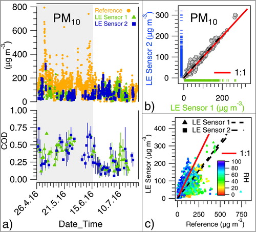
Table 1. Average (1σ ambient variability) of PM₁₀, PM_2.5, ambient temperature, relative humidity, and absolute humidity from the reference analyzers and the two Laser Egg (LE) sensors for the calibration period from 27 April 2016, until 25 July 2016. The number in bracket denotes one sigma ambient variability.

	PM10 (µg m^−3)	PM2.5 (µg m^−3)	Ambient temperature (°C)	Relative humidity (%)	Absolute humidity (g m^−3)
Reference	121.0 (87.1)	50.0 (33.0)	31.5 (3.9)	55.0 (22.4)	17.9 (6.0)
Laser Egg Sensor 1	62.8 (41.3)	51.6 (32.6)	32.8 (7.0)	23.4 (3.0)	7.4 (0.9)
Laser Egg Sensor 2	69.8 (45.2)	62.1 (39.5)	35.1 (7.5)	27.0 (3.4)	8.9 ( 1.0)

High nRMSE (∼73% for both sensors) indicated low accuracy of PM₁₀ measurements from the sensor. Additionally, the two sensors had an MBE of −38.2 µg m⁻³ and −44.9 µg m⁻³, respectively (Table 2), indicating that the LE monitor underestimates PM₁₀. RMA regression of all PM₁₀ measurements acquired during the calibration period from LE Sensors 1 and 2 with reference PM₁₀ reveals a moderate correlation with a slope of 0.62 and 0.61 and a Pearson correlation coefficient (r) value of 0.43 and 0.41 (Table 3), respectively.

Table 2. Table showing the Root Mean Square Error (RMSE), normalized Root Mean Square Error (nRMSE) and Mean Bias Error (MBE) computed for raw and post-correction PM₁₀ and PM_2.5 measurements obtained from Laser Egg sensors denoted as LES1 and LES2.

PM10
	Full Calibration Period (27 April–25 July 2016)		Summer season (27 April–15 June 2016)		Monsoon season (16 June–25 July 2016)
	Raw (LES1/LES2)	Post-correction (LES1/LES2)	Raw (LES1/LES2)	Post-correction (LES1/LES2)	Raw (LES1/LES2)	Post-correction (LES1/LES2)
RMSE (µg m^−3)	75.1/84.3	58.0/69.8	110.7/115.9	77.0/93.1	43.8/40.8	43.8/40.4
nRMSE (%)	73.6/72.3	56.8/59.9	75.3/77.7	52.4/61.8	57.0/46.7	57.0/46.1
MBE (µg m^−3)	−38.2/−44.9	−20.0/−18.1	−91.7/−87.3	−30.9/−23.2	−8.1/−8.6	−13.9/−13.6
PM2.5
	Full Calibration Period (27 April–25 July 2016)		Summer season (27 April–15 June 2016)		Monsoon season (16 June–25 July 2016)
	Raw (LES1/LES2)	Post-correction (LES1/LES2)	Raw (LES1/LES2)	Post-correction (LES1/LES2)	Raw (LES1/LES2)	Post-correction (LES1/LES2)
RMSE (µg m^−3)	31.0/37.9	27.5/32.2	26.1/35.3	29.4/34.4	34.1/40.7	26.1/29.6
nRMSE (%)	69.7/75.5	61.8/64.1	47.3/60.9	53.4/59.4	91.8/97.4	70.1/70.9
MBE (µg m^−3)	6.6/11.2	−1.9/1.3	−11.3/−4.2	−17.2/−12.4	19.1/28.3	8.7/16.5

Table 3. Value of the slope (S), intercept (I), and Pearson correlation coefficient (r) obtained from the regression of Laser Egg sensors (LE Sensor 1 and 2) with Reference (Ref) analyzers and inter-comparison of two LE sensors. % CV (coefficient of variation) depicts the relative precision between two LE sensors. RMA denotes Reduced Major axis regression, and OLS represents Ordinary Least Squares regression.

	PM10 (µg m^−3)	PM2.5 (µg m^−3)	Ambient temperature (°C)	Relative humidity (%)	Absolute humidity (g m^−3)
Comparison of Laser Egg (LE) Sensor with Reference (Ref) sensors
LE Sensor 1 = S × Ref + I	RMA	RMA	OLS	OLS	OLS
	S = 0.62 ± 0.01	S = 1.13 ± 0.02	S = 1.55 ± 0.03	S =0.08 ± 0.00	S = −0.05 ± 0.00
	I = 0	I = 0	I = −15.29 ± 0.95	I = 18.63 ± 0.23	I = (8.32 ± 0.9)×10^6
	r = 0.43	r = 0.54	r = 0.85	r = 0.56	r = −0.31
LE Sensor 2 = S × Ref + I	RMA	RMA	OLS	OLS	OLS
	S = 0.61 ± 0.01	S = 1.23 ± 0.03	S = 1.64 ± 0.04	S = 0.10 ± 0.00	S = −0.04 ± 0.01
	I = 0	I = 0	I = −16.76 ± 1.16	I = 21.57 ± 0.28	I = (9.62 ± 0.13)×10^6
	r = 0.41	r = 0.51	r = 0.88	r = 0.66	r = −0.23
Inter Laser Egg (LE) Sensor Comparison
LE Sensor 2 = S × LE Sensor 1 + I	RMA	RMA	OLS	OLS	OLS
	S =1.04 ± 0.01	S = 1.13 ± 0.01	S = 0.99 ± 0.01	S = 1.07 ± 0.01	S = 1.17 ± 0.01
	I = 0	I = 0	I = 1.76 ± 0.21	I = 2.52 ± 0.26	I = (0.1 ± 0.1) ×10^6
	r = 0.98	r = 0.98	r = 0.99	r = 0.98	r = 0.97
	CV = 7.9%	CV = 11.2%	CV = 3.2%	CV = 11.8%	CV = 11.8%

When hourly averaged PM₁₀ measurements from three identical original LE sensors were compared against a BAM for two months as part of a field evaluation carried out by SCAQMD at an ambient monitoring site in southern California, a similar underestimation, but with a lower r-value (0.2) was reported (SCAQMD 2016). Though the results of the SCAQMD study are preliminary, they reinforce the point that LE monitors do not provide a very accurate measure of ambient PM₁₀ mass concentration. Another low-cost sensor, the AlphaSense OPC-N2, underestimated PM₁₀ (slope of ∼0.2 from OLS, r = 0.7–0.9) compared to reference β-attenuation monitors during a field-calibration at a site characterized by heavy dust loading in California (Mukherjee et al. 2017).

During the two severest dust storms observed during the calibration period on 2 May, 2016, 21:00 Local Time (LT) and 11 June 2016, 21:00 LT, the hourly averaged PM₁₀ mass concentration reported by the reference analyzer was 794 µg m⁻³ and 741 µg m⁻³, respectively while the LE sensors reported 120 µg m⁻³ and 38.4 µg m⁻³ (Figure 1c), respectively. Likewise, a field study carried out in Salt Lake City, Utah reported that Plantower PMS sensors that also work on the principle of laser-based light scattering are not very accurate at measuring PM₁₀ when the ambient PM contains a higher coarse fraction (Sayahi, Butterfield, and Kelly 2019), particularly during dust storm events, when the reference Tapered Element Oscillating Microbalance (TEOM) reported ∼472 µg m⁻³ while the low-cost sensor reported a mass concentration <50 µg m⁻³.

A scatter plot of PM₁₀ measurements from the two LE sensors reveals a slope of 1.04 (Table 3) and an r-value of 0.98, indicating high precision, while a low average CV of 7.9% showed that the measurements were highly reproducible and in compliance with the US EPA standard of CV less than 10% between identical units (EPA 2015). The LE PM₁₀ measurements were more precise than those of another low-cost sensor, the Alphasense OPC-N2, which reported an average CV of ∼22% during a field campaign in the UK (Crilley et al. 2018).

The bottom panel of Figure 1a shows the daily average value of the COD for the two LE sensors. Vertical bars represent the daily variability of the COD as the 75^th and 25^th percentiles. The daily average value of the COD for PM₁₀ from the two low-cost sensors varied from 0.3 to 0.6 during the days (27 April 2016 to 15 June 2016) with low to moderate levels of ambient RH^Ref and high wind speeds (Figure S3). However, from 16 June 2016, with an increase in RH^Ref and AH^Ref and a decrease in wind speeds, PM₁₀ reported by the low-cost sensors became more homogeneous to the reference analyzer with the daily average COD varying from 0.1 to 0.3 which indicates that the accuracy of PM₁₀ measurements from the LE was affected by particle size distribution, possibly wind speed and ambient RH.

PM_2.5 measurements

Figure 2a (top panel) shows the hourly averaged PM_2.5 mass concentration obtained from the reference β-attenuation analyzer (circular markers in orange) and the two LE sensors (green triangular and blue square markers) for the period of 27 April 2016 to 25 July 2016. The ambient PM_2.5 mass loadings reported by the reference analyzer, and LE Sensors 1 and 2, varied from <1 to 228 µg m⁻³, 2.8 to 211.2 µg m⁻³, and 3.2 to 267.8 µg m⁻³, respectively. The average (1σ ambient variability) for PM_2.5 during the calibration period was 50.0 (33.0) µg m⁻³, 51.6 (32.6) µg m⁻³, and 62.1 (39.5) µg m⁻³, as measured by the reference analyzer and LE Sensor 1 and Sensor 2, respectively (Table 1). The RMA of all PM_2.5 measurements acquired from LE Sensors 1 and 2 versus PM_2.5 from the reference analyzer during the calibration period reveal a moderate correlation with an r-value of 0.54 and 0.51 (Table 3, Figure 2c), respectively, which was comparable to few low-cost PM sensors namely Dylos, Shinyei PPD60PV, Shinyei PPDD42NS (Jiao et al. 2016) and AlphaSense (Crilley et al. 2018) but lower than many optical sensors such Panasonic PM_2.5 senor (Nakayama et al. 2018), Nova SDS011 (Liu et al. 2019), Shinyei PPD42NS (Holstius et al. 2014), Plantower PMS7003 (Wang et al. 2019), Plantower PMS3003 (Zheng et al. 2018). When hourly averaged PM_2.5 measurements from three identical original LE sensors were compared against BAM for two months as a part of field evaluation carried out by SCAQMD at an ambient monitoring site in southern California, a higher r-value of 0.8 was reported (SCAQMD 2016).

Figure 2. (a, top) Time series plot of hourly averaged PM_2.5 mass concentration from the reference analyzer (circular markers in orange) and two Laser Egg (LE) sensors (green triangular and blue square markers, respectively) for the period from 27 April 2016 to 25 July 2016. The shaded portion represents the dry summer period (27 April 2016–15 June 2016) with average RH varying from 9% to 58% while the unshaded portion represents the wet monsoon period (16 June 2016–25 July 2016) with average RH varying from 61% to 85%. (a, bottom) The daily average value of the coefficient of divergence (COD) for raw PM_2.5 measurements from the LE sensors. Vertical bars represent the daily variability as the 75^th and 25^th percentiles of the COD. (b) Reduced Major Axis (RMA) regression of PM_2.5 from LE Sensor 2 versus Sensor 1. Marginal rugs have been added to show the distribution of data. (c) RMA regression of PM_2.5 from the LE sensors versus the reference analyzer. Markers are color-coded according to ambient RH.

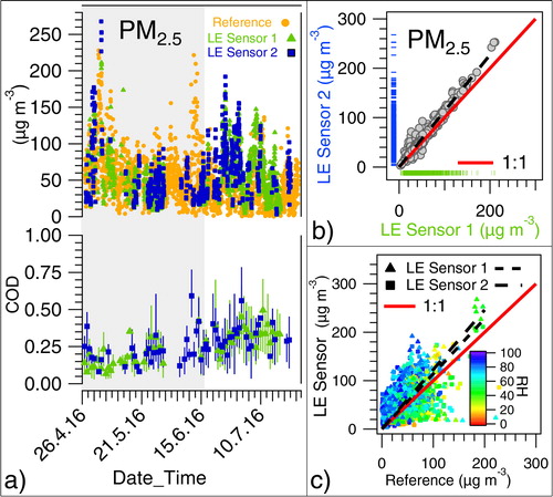
A scatter plot of PM_2.5 measurements from the two LE sensors reveals a slope of 1.13 and an r-value of 0.98, indicating that Sensor 2 moderately overestimated PM_2.5 when compared to Sensor 1 (Table 3, Figure 2b). In this context it is worth noticing that the AH^LE within the outer casing of the LE is always significantly lower than the ambient AH^Ref (Figure S9c in the online SI), indicating that the outer casing may be acting as a dryer and that the outer casing of Sensor 2 had a 5–10% higher RH inside the unit than Sensor 1 (Figure S9a in SI). Hence the difference might primarily be driven by differences in the aerosol wet diameter within the two units. A scatter plot of PM_2.5 measurements from the two LE sensors versus the reference analyzer reveals a slope of 1.13 and 1.23 (Table 3), indicating overestimation. Field evaluations carried out in India (Zheng et al. 2018), China (Barkjohn et al. 2020), and USA (Kelly et al. 2017; SCAQMD 2019) also report the tendency of PMS3003 sensors to overestimate ambient PM_2.5 mass concentrations when compared to FEM measurement techniques.

A CV of 11.2% between the PM_2.5 measurements from the two LE sensors was comparable to that obtained from the Plantower PMSA003 during a field study in Baltimore, Maryland (Levy Zamora et al. 2019) and lower (more precise) than that of another low-cost sensor, the Alphasense OPC-N2, which reported an average CV of ∼25% during a field campaign in the UK (Crilley et al. 2018). However, PM_2.5 measurements from the LE monitors did not meet the US EPA standard of CV less than 10% between identical units (EPA 2015). It seems that the sensor performance could be improved by placing a dryer in the outer casing of both units.

The bottom panel of Figure 2a shows the daily average value of COD for the two LE sensors. Vertical bars represent the daily variability of the COD as the 75^th and 25^th percentiles. The daily average value of COD for the two LE sensors varied from 0.1 to 0.3 during the days (27 April 2016 to 15 June 2016) with low levels (<40%) of RH^Ref (Figure S3), indicating high homogeneity in PM_2.5 measurements. However, from 16 June 2016, with an increase in RH^Ref and AH^Ref, the PM_2.5 measurements from the LE became more heterogeneous in comparison to the reference, with the daily average COD varying from 0.2 to 0.4, which indicates that ambient RH influences the accuracy of PM_2.5 measurements from LE monitors.

Impact of aspiration losses on Laser Egg (LE) accuracy

Particles entering the outer casing of the LE must make a 90° turn with respect to the ambient horizontal wind direction, as is normal for all down-facing inlets. Particle losses are proportional to the particle stokes number (Stk) and the ratio between the external (Uo) and internal (U) velocity of the carrier gas and are hence expected to be larger for larger particles and higher wind speeds.

Hangal and Willeke (1990) gave the following expression for the aspiration efficiency of a 90° sampling inlet: (7) $$\mathit{Aspiration}\mathrm{ }\mathit{efficiency}=1-3\times {\mathit{Stk}}^{\sqrt{\frac{U}{U_o}}}$$(7) where $\mathit{Stk}$ is the particle stokes number given as (8) $$\mathit{Stk}=\mathrm{ }\frac{{\rho }_{p{d}_{p\mathrm{ }}^2}{U}_o}{18\mu D}$$(8) and U is the inlet velocity, Uo is the wind speed, dp is the particle diameter, $\rho$ is the particle density, µ is the air viscosity, and D is the characteristic inlet dimension.

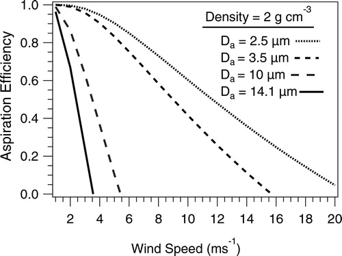
Figure 3 shows the aspiration efficiency of the LE inlet as a function of the wind speed for particles with varying aerodynamic diameters. It is evident that smaller particles have larger aspiration efficiency at any given wind speed. Moreover, for the inlet sampling configuration of the LE monitor, a particle with an aerodynamic diameter of 10 µm, which corresponds to an optical equivalent diameter of 6 to 7 µm for mineral dust, will not be aspirated into the detection chamber beyond external wind speeds of 6 ms⁻¹. Therefore, the LE monitor is expected to underestimate PM₁₀ in comparison to the reference analyzer (which has close to 100% inlet efficiency for the full ambient wind speed range), particularly when the PM₁₀ aerosol is dominated by coarse mode dust particles and wind speeds are high. However, at the average wind speeds (4.1 to 6.8 ms⁻¹) observed in our study period, the LE measures PM₁₀ thanks to its modified inlet.

Figure 3. Aspiration efficiency of the Laser Egg (LE) inlet as a function of external wind speed (U_o) for particles with varying aerodynamic diameters (D_a) and a density of 2 g cm⁻³.

So far, only two other studies (Mukherjee et al. 2017; Sayahi, Butterfield, and Kelly 2019) have looked at the impact of wind speed on PM measurements from low-cost sensors. Mukherjee et al. (2017) reported that the Airbeam (a low-cost OPC) underestimated PM_2.5 compared to the GRIMM (reference OPC) when wind speeds were between 1 to 3 ms⁻¹ but overestimated at higher wind speeds, which is opposite to what we observe in our study, and possibly related to the blunt shape of the Airbeam sensor. Vanderpool et al. (2018) reported sampling effectiveness above 100% for super isokinetic sampling and below 100% for sub isokinetic sampling with a blunt PQTSP sampler in a wind tunnel study. Another study (Sayahi, Butterfield, and Kelly 2019) did not explicitly analyze the impact of wind speed on the accuracy of PM measurements, but instead observed the direct correlation between hourly averaged PM_2.5 and PM₁₀ measured from Plantower PMS (PMS1003 and PMS5003) sensors and wind speed (varied between 0.08 to 5.9 ms⁻¹) and found no discernible trend (r² <0.138) during a long-term field evaluation carried out at Salt Lake City, Utah from 2016 to 2017.

In a field evaluation study of several low-cost PM_2.5 sensors carried out in Atlanta (USA) and Hyderabad (India), Johnson et al. (2018) used a single 25 mm DC fan (reported flow of 67 LPM) at the inlet of a box housing a single sensor, and three 25 mm fans for another box housing five low-cost sensors. However, they did not evaluate the impact of fan flow rate and ambient wind speed on particle losses. As per the expression by Hangal and Willeke (1990), assuming similar fan dimensions, a particle of 2.5 µm aerodynamic diameter would still have an aspiration efficiency of 0.44 in the Johnson et al. (2018) inlet at high wind speeds of ∼13 ms⁻¹ with a fan flow rate of 67 LPM, but in our study, which uses an accessory fan with a lower flow rate of 40 LPM, a particle of 2.5 µm diameter has an aspiration efficiency of only 0.18 at that wind speed.

Impact of aerosol density on Laser Egg (LE) accuracy

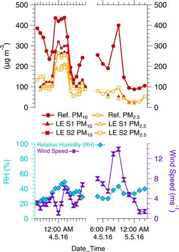
Figure 4 shows the hourly averaged PM₁₀ and PM_2.5 measurements from the reference and the two LE sensors during two dust storms observed from 3 May 2016, 17:00:00 to 4 May 2016, 08:00:00 and 4 May 2016, 17:00:00 to 5 May 2016, 02:00:00, respectively, with a peak PM₁₀ mass loading of ∼450 µg m⁻³. During the first storm, high dust loading due to long-range transport of desert dust coincided with low local wind speeds while the second storm was characterized by higher wind speeds. The average wind speeds during the first dust storm (4–6 ms⁻¹) ensured that the optical system received only PM10 aerosol, as the aerodynamic cutoff of the modified LE inlet system is 10 µm (Figure 3). However, an overestimation of PM_2.5 mass concentration and simultaneous underestimation of PM₁₀ by the LE monitor is evident during the first dust storm under conditions with no confounding errors from wind speed or RH.

Figure 4. (Top) PM₁₀ (solid markers) and PM_2.5 (hollow markers) measurements from the reference and the two Laser Egg (LE) sensors during two dust storms observed from 4 May 2016, 17:00:00 to 4 May 2016, 08:00:00 and 5 May 2016, 17:00:00 to 5 May 2016, 02:00:00, respectively. (Bottom) Relative Humidity (RH) and wind speed during the two dust storm periods.

It appears that the LE low-cost sensor assumes the optical equivalent diameter (d_o) to be the same as the aerodynamic equivalent diameter (d_a), and therefore ends up attributing a higher fraction of aerosol mass to the PM_2.5(da) size fraction than the reference analyzer, which cuts based on aerodynamic diameter. This error probably stems from the fact that low-cost sensors are generally factory calibrated using polystyrene spherical latex particles, which have a density of 1.05 g cm⁻³ (Mukherjee et al. 2017; Nakayama et al. 2018; Zhang, Marto, and Schwab 2018).

During pre-monsoon season, particles in the size range 0.7–2.5 µm are dominated by clay minerals (Singh et al. 2004) with an effective density of ∼2 g cm⁻³. Assuming the optical diameter (d_o) to be the same as the volume equivalent diameter (d_veq), the aerodynamic diameter (d_a) of a 2.5 µm clay particle is ∼3.5 µm, as per the following expression (Chien et al. 2016; Murphy et al. 2004) (9) $$d_a=d_o\sqrt{\rho }$$(9) where $\rho$ is the particle density.

The LE measures PM_3.5 but converts volume to mass using a density of 1.05 g cm⁻³ instead of 2 g cm⁻³. The two errors partially cancel each other out, resulting in what appears to be a better accuracy for LE PM_2.5 measurements under dry high dust conditions. Nevertheless, it can be seen from Figure 4 that at average wind speeds, the clay mode with an aerodynamic diameter of 2.5–3.5 µm and optical diameter of less than 2.5 µm results in a slight overestimation of the PM_2.5 mass by the LE. At high wind speeds (>10 ms⁻¹), the aerodynamic inlet cutoff of the modified LE drops below 3.5 µm and approaches 2.5 µm for the peak wind speeds of 12 ms⁻¹ observed during the second dust storm. Under these conditions, the LE underestimates the PM_2.5 mass thanks to the lower density of 1.05 g cm⁻³, rather than 2 g cm⁻³, used to convert volume to mass, even though both the LE and the reference sensors measure PM_2.5 at high wind speeds.

Serious underestimation of the PM₁₀ mass under conditions with average wind speeds can also be explained by the assumption that the LE monitor uses a sub-optimal value of aerosol density. The inlet cutoff at average wind speeds is close to d_a=10 µm, and hence both the reference and the low-cost sensors measure PM₁₀. However, the LE converts volume to mass using a density of 1.05 g cm⁻³ rather than 2 g cm⁻³ and hence underestimates the PM₁₀ mass.

Impact of relative humidity (RH) on Laser Egg (LE) accuracy

The reference PM analyzers use an inlet heating system to regulate the sample RH to ∼40% and, therefore measure the dry mass of the aerosol. However, semi-volatile aerosol species such as ammonium nitrate and ammonium chloride, which are in a temperature- and RH-dependent equilibrium with the gas phase, can partition from the aerosol phase into the gas phase due to this heating. On the other hand, in the absence of humidity control in the LE monitor, this technique determines aerosol mass using the wet diameter of the aerosol, which can be up to three times larger than the dry diameter and varies as a function of RH. Therefore, a variation in the accuracy of the LE monitor’s PM measurements with varying RH is expected because of the fundamental difference in both techniques.

Several field studies on optical low-cost sensors have reported an inherent positive bias in PM measurements with respect to FEM analyzers at high RH in the past (Badura et al. 2018; Crilley et al. 2018; Jayaratne et al. 2018; Levy Zamora et al. 2019; Liu et al. 2019; Nakayama et al. 2018; Zheng et al. 2018). Figures 1c and 2c show that as the RH^Ref increases to more than 80%, the LE monitor overestimates both PM₁₀ and PM_2.5 when compared to the reference analyzers, indicating the impact of RH on the LE monitor’s accuracy. Likewise, the markers representing low ambient RH^Ref conditions lie mostly below the solid (red) 1:1 line in the scatter plot.

Correction for the biases introduced by particle density, hygroscopic growth, and aspiration efficiency losses in Laser Egg (LE) PM measurements

The following corrections were applied successively to correct the LE monitors’ PM measurements:

1. Particle density correction: The calibration period was split into summer (27 April to 15 June 2016) and monsoon (16 June to 25 July, 2016) based on the levels of ambient RH. Assuming an average particle density of 2 g cm⁻³ and 1.2 g cm⁻³ during the summer and the monsoon, respectively, the raw PM₁₀ and PM_2.5 measurements were corrected as: (10) $$\mathbf{During} \mathbf{summer}:\mathit{Laser}\mathrm{ }\mathit{Egg}\text{ PM }\left(\text{Density corrected}\right)=\frac{\mathit{Raw}\mathrm{ }PM\mathrm{ }\times 2\mathrm{ }{g\mathrm{ }cm}^{-3}}{1.05\mathrm{ }{g\mathrm{ }cm}^{-3}}$$(10) (11) $$\mathbf{During} \mathbf{monsoon}:\mathit{Laser}\mathrm{ }\mathit{Egg}\text{ PM }\left(\text{Density corrected}\right)=\frac{\mathit{Raw}\mathrm{ }PM\mathrm{ }\times 1.2\mathrm{ }{g\mathrm{ }cm}^{-3}}{1.05\mathrm{ }{g\mathrm{ }cm}^{-3}}$$(11) where 1.05 g cm⁻³ represents the density of polystyrene latex spheres commonly used to calibrate optical sensors. Nakayama et al. (2018) used a factor of 1.3 to correct for the density of PM_2.5 measurements from an optical sensor by assuming particle density between 1.2 and 1.8 g cm⁻³.

2. Hygroscopic growth correction: To correct for the positive bias in PM measurements of the LE under high RH, it was assumed that the ambient aerosol follows a growth curve identical to that of secondary organic aerosol formed from the oxidation of cyclopentene which has a growth factor of 1.20 at 90% RH (Varutbangkul et al. 2006). (12) $$PM\mathrm{ }\left(RH\mathrm{ }\mathit{corrected}\right)=\frac{PM\mathrm{ }\left(\mathit{Density}\mathrm{ }\mathit{corrected}\right)}{{\left[1+\mathrm{ }{(1-a_w)}^{-0.4428}\times 0.0841\times a_w^{1.2347}\right]}^3}$$(12)

   where (13) $$a_w=\mathrm{ }\frac{{RH}^{\mathit{Ref}}}{100}$$(13)

3. Correction for aspiration losses and incorrect cutoff diameter: The interaction between external wind speeds and particle size distribution decreases the accuracy of the modified LE PM sensor. Figures S4a and S4b in the online SI show the observed ratio of the LE PM (after density and RH correction) to the reference PM plotted as a function of external wind speeds for the summer season (27 April–15 June 2016) during the calibration period. To correct for the aspiration losses and incorrect cutoff diameter, we assume a bimodal aerosol volume size distribution (Figure S4c), which peaks at 0.25 µm and 2.5 µm optical diameter and has a uniform density of 2g cm⁻³ during the summer season. This assumption is reasonable and represents a substantial clay burden present in the coarse mode aerosol during the pre-monsoon season. The assumed particle size distribution fits the observed PM_2.5/PM₁₀ ratio of the reference analyzer during dust episodes. The equivalent optical cutoff diameters for the reference PM_{10 (da)} and PM_{2.5 (da)} analyzers are 7.07 µm and 1.77 µm for a particle density of 2 gcm⁻³. Thus, while the reference analyzers measure the area under the black curve until 1.77 (PM_2.5) and 7.07 µm (PM₁₀), the LE sensors misattribute extra aerosol from 1.77 µm to 2.5 µm as PM_2.5 and from 7.07 µm to 10 µm as PM₁₀. Moreover, while the reference analyzer is immune to aspiration losses, the various colored curves represent the fraction of aerosol aspirated into the LE monitors at different wind speeds.

Thus, the ratio of the area under the curves of the assumed aerosol size distribution (Figure S4c in the SI) as measured by the LE monitor and reference analyzer in accordance with their respective cutoffs and the aspiration losses (wind speed) gives us a theoretical ratio shown by the maroon markers (Figures S4a and b in the SI). The LE PM measurements are then corrected for both aspiration-related losses and incorrect cutoff diameter as (14) $$PM\mathrm{ }\mathit{corrected}\mathrm{ }\mathit{for}\mathrm{ }\mathit{aspiration}\mathrm{ }\mathit{loss}\mathrm{ }\mathit{and}\mathrm{ }\mathit{cut}-\mathit{off}\mathrm{ }\mathit{diameter}=\frac{\mathit{Density}\mathrm{ }\mathit{and}\mathrm{ }RH\mathrm{ }\mathit{corrected}\mathrm{ }PM}{f\left(\mathit{Wind}\mathrm{ }\mathit{speed}\right)}$$(14) where f(Wind speed) has been calculated after fitting a sigmoidal curve (maroon curve in Figures S4a and b in the SI) through the theoretical aspiration losses derived from the assumed aerosol size distribution (Figure S4c). The red and blue curves in Figures S4a and b show similar theoretical curves for aspiration losses derived from particle size distributions observed at Kanpur (Figure S4d) (Kaskaoutis et al. 2012) and Gual Pahari (Figure S4e) (Hyvärinen et al. 2011) in India, while the yellow curve represents another theoretical correction curve derived from a different assumed low-dust size distribution shown in Figure S4f.

It can be seen from Figures S4a-f and the accompanying Table S2 that the exact position of the coarse mode barely impacts the correction for PM_2.5 shown by the overlapping blue, red, and maroon curves in Figure S4b. The correction for PM_2.5 in the presence of a significant coarse mode is impacted only by the assumed density, which widens or closes the gap between the d_o=2.5 µm and d_a=2.5 µm as can be seen in Figures S5b and S6b, which assume a density of 1.2 g cm⁻³ and 2.7 g cm⁻³ for the ambient aerosol. The correction for PM₁₀ is very sensitive to the exact position of the coarse mode peak, as can be seen by the correction curves derived from different size distributions in Figure S4a which limits the usefulness of the LE monitor for measuring PM₁₀.

During the monsoon season, aerosol loading comprising primarily combustion-derived aerosol, primary and secondary organic aerosol, secondary inorganic aerosol and a small coarse mode dominated by primary biological particles with an average density of 1.2 g cm⁻³ can be represented using a hypothetical size distribution with low dust loading (Figure S5f in the online SI). Aspiration losses occurring during the monsoon season were corrected using a similar algorithm as that for the summer season using the size distribution depicted in Figure S5f in the SI.

Laser Egg (LE) PM measurements post-correction

Figure 5 shows the correlation plots of the LE PM versus the reference PM obtained after performing RMA regression for raw LE measurements (a and d), after RH and density correction (b and e), and after correcting for aspiration losses and cutoff diameter (c and f). The solid (red) line indicates the 1:1 line. Figure S7 in the online SI shows the time series of hourly averaged PM₁₀ and PM_2.5 measured by the reference and LE sensors for the period between 27 April 2016 and 25 July 2016, before and after correction. Corrections reduced the RMSE by ∼22.8% (from 75.1 µg m⁻³ to 58.0 µg m⁻³) and 17.2% (from 84.3 µg m⁻³ to 69.8 µg m⁻³) for PM₁₀ measurements from LE Sensor 1 and Sensor 2, respectively, for the entire calibration period. The MBE in the LE monitor’s PM₁₀ measurements decreased from −38.2 µg m⁻³ and −44.9 µg m⁻³ to ∼−20.0 µg m⁻³and ∼−18.1 µg m⁻³ for Sensor 1 and Sensor 2, respectively (Table 2). The slope obtained from the RMA regression of the LE monitor’s PM₁₀ versus the reference PM₁₀ increased from 0.6 (for raw measurements) to 0.83 and 0.89 for Sensor 1 and Sensor 2, respectively, after both corrections were applied, while the r-value increased from 0.43 and 0.41 to 0.67 and 0.61 (Figure 5), indicating improvement in both linearity and accuracy. Specifically, during the summer period (27 April to 15 June, 2016) characterized by low RH and high dust loading (average PM₁₀ = 149 µg m⁻³), the MBE in the LE monitor’s PM₁₀ measurements decreased from ∼−90 µg m⁻³ to −30.9 µg m⁻³ (Sensor 1) and −23.2 µg m⁻³ (Sensor 2) after correcting for density and aspiration losses (Table 2).

Figure 5. Correlation plots of the Laser Egg (LE) PM versus the reference PM obtained after performing reduced major axis (RMA) regression for raw LE measurements (a and d), after RH and density correction (b and e), and after correcting for aspiration losses and cutoff diameter (c and f). The solid (red) line indicates the 1:1 line. In each of the above plots, “S” refers to the slope of the best–fit line, and “r” refers to the Pearson correlation coefficient. The markers are color-coded according to ambient RH.

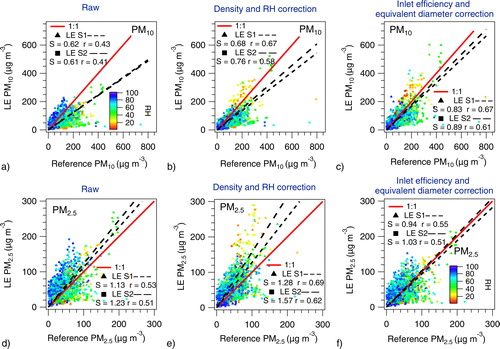
Overall, after the application of both corrections, the RMSE in the LE monitor’s PM_2.5 measurements decreased by ∼11.3% (from 31.0 µg m⁻³ to 27.5 µg m⁻³) and ∼15% (from 37.9 µg m⁻³ to 32.2 µg m⁻³) for Sensor 1 and Sensor 2, respectively. The slope obtained from the RMA regression of PM_2.5 measurement from the LE monitor versus the reference decreased from 1.13 and 1.23 for raw measurements to 0.94 and 1.03 post-correction for LE Sensor 1 and Sensor 2, respectively (Figure 5). Specifically, during the monsoon period (16 June to 25 July 2016) characterized by high RH, where the LE monitor has a tendency to overestimate PM_2.5 due to lack of inlet heating, the MBE in the LE monitor’s PM_2.5 measurements decreased from 19.1 µg m⁻³ to 8.7 µg m⁻³ and 28.3 µg m⁻³ to 16.5 µg m⁻³ for Sensor 1 and Sensor 2, respectively, after corrections (Table 2).

Overall, post-corrections, the accuracy of the LE monitor’s PM measurements increased, indicated by a slope varying between 0.83 and 1.03 (Figure 5) obtained after performing RMA regression with the reference PM and a low MBE of <20 µg m⁻³ (PM₁₀) and <3 µg m⁻³ (PM_2.5) (Table 2). The modified version of the LE monitor could thus be used for ambient monitoring provided accurate RH and wind speed measurements, and knowledge about the site’s aerosol size distribution during high dust periods are available.

Ambient temperature measurements

The average (1σ ambient variability) of ambient temperature during the calibration period (27 April 2016 to 25 July 2016) was 31.5 (3.9)°C, 32.8 (7.0) °C and 35.1 (7.5) °C as measured by the reference Met One 064 Air Temperature sensor, and the LE Sensor 1 and Sensor 2, respectively (Table 1). Inter-comparison of the temperature measurements reveals high precision in the LE sensors (r = 0.99, CV = 3.2%); however, they had an offset of ∼1.8 °C among themselves (Table 3).

Figure 6a shows the diel plot of ambient temperature measurements obtained from the reference sensor (circular markers in orange) and the two LE monitors (green triangular and blue square markers) during the calibration period. The markers connected by lines indicate the hourly average, and the shaded portion represents the ambient variability as the 75^th and 25^th percentiles. Qualitatively, the diurnal trend of temperature from the reference sensor and the LE monitors looks similar, characterized by a daytime maximum between 14:00 to 15:59 LT and minima between 05:00 to 05:59 LT. However, it is evident that the LE overestimates the ambient temperature by ∼5 to 10 °C between 06:00 to 18:59 LT and underestimates the temperature by ∼0.5 to 2 °C between 19:00 to 05:59 LT.

Figure 6. (a) Diel plot of ambient temperature from the reference analyzer (circular markers in orange) and two Laser Egg (LE) sensors (green triangular and blue square markers, respectively) for the calibration period. The markers connected by lines indicate the hourly averages, and the shaded portion represents the ambient variability as the 75^th and 25^th percentiles. (b) Time series plot of hourly averaged ambient temperature from the reference and the LE sensor plotted along with solar radiation measurements (hollow circular markers) from 13 July 2016 to 15 July 2017.

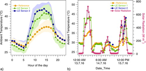
In the LE monitor, the temperature sensor lies inside the body/chamber, making it susceptible to heat given off by the circuitry, which the manufacturer blames for the discrepancies between the reference and the LE temperature measurements. However, it seems that the overestimation in temperature is due to the absorption of SR by the LE monitor’s casing. This hypothesis is validated by looking at a time series plot of hourly averaged temperature measurements from the reference, and LE sensors plotted along with SR on the secondary axis (Figure 6b) from 13 July 2016, to 15 July 2016. 13 July 2016 being a clear day with maximum daytime SR ∼700 W m⁻², the LE monitor overestimated the daytime temperature by ∼9 °C, while on 14 July 2016, an overcast day with average daytime SR of only ∼300 W m⁻², the difference between the LE monitor and the reference temperature sensor decreased to less than 2 °C. 15 July 2016 was a partially overcast day, and as the average SR increased until 11:00 LT, the sensors overestimated temperature by ∼6 to 8 °C. However, with a sharp dip in SR from 550 W m⁻² to 180 W m⁻² because of cloud cover between 11:00 to 12:00 LT, the LE sensors simultaneously cooled down and the deviation in temperature decreased to ∼2 °C. After 12:00 LT, as the SR increased, the LE temperature simultaneously heated up again. A field study carried out by SCAQMD (SCAQMD 2019) in California, United States reported better accuracy and an r-value of 0.98 between temperature measurements obtained from the Laser Egg 2+ (a new model of LE) and the SCAQMD meteorological station when the ambient temperature varied between ∼2 °C and 35 °C. This behavior confirms that the absorption of SR by the modified casing of the LE monitor is the primary cause for higher-than-average daytime temperature measurements.

Figure S8 in the online SI shows that the temperature deviation of the LE sensor can be explained as a function of SR during the day and ambient RH (a proxy for evaporative cooling) at night. Provided accurate measurements of SR and RH^Ref from co-located sensors are available, the biased temperature measurements T^LES1, T^LES2 from the LE Sensor 1 and Sensor 2, respectively, can be corrected using the following multiple linear regression equations: (15) $$T^{\mathit{Ref}}=0.43\mathrm{ }\times T^{\mathit{LES}1}-0.003\times SR-0.064\times {RH}^{\mathit{Ref}}\mathrm{ }+21.50\mathrm{ }\left(r_{\mathit{adj}\mathrm{ }}^2=0.83\right)$$(15) (16) $$T^{\mathit{Ref}}=0.47\mathrm{ }\times T^{\mathit{LES}2}-0.003\times SR-0.049\times {RH}^{\mathit{Ref}}+18.77\mathrm{ }\left(r_{\mathit{adj}\mathrm{ }}^2=0.84\right)$$(16)

Relative humidity (RH) measurements

Figure S9a and b in the online SI show the hourly averaged time series and diel profile of the RH measurements from the reference Met One 083E RH sensor and the two LE sensors. During the calibration period, the average RH (1σ ambient variability) was 55.0 (22.4)% from the reference and 23.4 (3.0)% and 27.0 (3.4)% from the two LE sensors, respectively (Table 1). The LE underestimated RH by more than 50%. OLS of RH from the LE sensors versus the reference reveals only a moderate correlation, with an r-value of 0.56 and 0.66 (Table 3). Inter-comparison of the RH measurements from the two LE sensors reveals moderate precision, with CV = 11.8% (Table 3). The SCAQMD field study (SCAQMD 2019) reported better accuracy and an r-value of 0.99 between RH measurements obtained from the Laser Egg 2+ and the SCAQMD meteorological station when the ambient RH varied between ∼15% to 100%.

To ascertain if the LE sensors’ inaccurate RH levels were caused by their inaccurate temperature measurements, we converted the RH^Ref and RH^LE to corresponding AH^Ref and AH^LE using the accurate reference temperature ($T^{\mathit{Ref}}$) in both cases and compared the two. (17) $${AH}^{\mathit{Ref}}\mathrm{ }\left(g\mathrm{ }{m}^{-3}\right)=\frac{es\times {RH}^{\mathit{Ref}}\mathrm{ }\times 18\mathrm{ }{g\mathrm{ }\mathit{mol}}^{-1}}{100\times (8.314\mathrm{ }J\mathrm{ }{K}^{-1}{\mathrm{ }\mathit{mol}}^{-1}\mathrm{ }\times \left(T^{\mathit{Ref}}+273.15\right)}$$(17) (18) $${AH}^{LE}\mathrm{ }\left(g\mathrm{ }{m}^{-3}\right)=\frac{es\times {RH}^{LE}\mathrm{ }\times 18\mathrm{ }{g\mathrm{ }\mathit{mol}}^{-1}}{100\times \left(8.314\mathrm{ }J\mathrm{ }{K}^{-1}{\mathrm{ }\mathit{mol}}^{-1}\right)\mathrm{ }\times \left(T^{\mathit{Ref}}+273.15\right)}$$(18) where e_s is the saturation vapor pressure estimated as per the expression by Alduchov and Eskridge (1996) (19) $$es=610.94\mathrm{ }\times \exp \left(\frac{17.625\mathrm{ }\times \mathrm{ }{T}^{\mathit{Ref}}}{243.04\mathrm{ }+\mathrm{ }{T}^{\mathit{Ref}}}\right)\text{ Pa}$$(19)

Figures S9c and d in the SI show the hourly averaged time series and diel profile of the AH estimated from the reference RH sensor and LE monitors, respectively. While the reference analyzer reported a wide variation in AH from 5 to 25 g m⁻³, the AH from the LE monitors varied only between 2 and 12 g m⁻³ during the calibration period. It is again evident that the LE underestimated AH by almost 50% (Table 1) and did not capture its ambient variability. This suggests that the bias in the LE monitor’s RH sensor was independent of its biased temperature sensor. The RH sensor’s placement inside the outer casing could be responsible for the lower accuracy of RH measurements. It is possible that the outer casing not only absorbs solar radiation but is also hygroscopic and acts as a dryer, as the LE Sensor 1 with the lower measured AH (Figure S9c) also showed a lower overestimation of the measured PM_2.5 due to aerosol hygroscopic growth (Figure 5d). OLS between the reference AH and the LE monitor AH revealed a poor anti-correlation, with an r-value of −0.31 and −0.23 (Table 3).

As such, RH measurements from the LE do not quantitatively correspond to the ambient RH levels.

Future work and conclusion

In this article, we focus on the field calibration of a modified version of LE, a commercially available low-cost PM sensor that works on the principle of laser-based light scattering. Two identical LE monitors with modified casings to shield them from sunlight and rain and an accessory inlet fan were co-located next to the inlets of PM₁₀ and PM_2.5 β-attenuation reference analyzers at the IISER Mohali Atmospheric Chemistry Facility, a suburban site in the NW-IGP during a 3-month period from 27 April 2016 to 25 July 2016, and their performance was evaluated for regular ambient usage.

1. Measurements of PM₁₀, PM_2.5, ambient temperature, and RH from the LE monitor were always precise, with r > 0.9 and CV <12% for each inter-species correlation among the two sensors.

2. The average (1σ ambient variability) of PM₁₀ during the calibration period was 121.0 (87.1) µg m⁻³, 62.8 (41.3) µg m^−3, and 69.8 (45.2) µg m⁻³ as measured by the reference analyzer, and the LE Sensor 1 and Sensor 2, respectively. High nRMSE (∼73% for both sensors) and an MBE of −38.2 µg m⁻³ (Sensor 1) and −44.9 µg m⁻³ (Sensor 2) indicated low accuracy and underestimation of PM₁₀ measurements by the LE monitor.

3. This study highlights the effects of hygroscopic growth, aerosol density, aspiration losses of particles at high wind speeds, and the implications of assuming optical equivalent diameter to be the same as aerodynamic diameter on the accuracy of PM measurements acquired from low-cost sensors. While the study also presents methods to correct for the biases mentioned above, the end goal should be to ensure that the low-cost sensor reports accurate PM measurements to the targeted end-user rather than requiring complicated post-processing. Assessing personal exposure to PM using a sensor that underestimates ambient PM levels under certain conditions can also have a detrimental effect on people’s health. For instance, in the dust storms (average wind speeds of 9 ms⁻¹, solar radiation of 400 Wm⁻² and reference PM₁₀ >200 ug m⁻³) observed during daytime in the calibration period, the average LE PM₁₀ levels (59 ug m⁻³) were about five times lower than those of the reference PM₁₀ analyzer (278 ug m⁻³) thus creating a false sense of air being clean to a person relying on LE for personal air quality monitoring. This false perception of clean and fresh air may be further amplified by dips in temperature and increases in wind speed commonly observed during dust storms, possibly prompting the user to schedule outdoor activity during such hours. Hence future development of low-cost PM sensors must focus on an inlet design that minimizes aspiration losses, better placement of the RH and temperature sensor outside the casing to avoid artifacts, and using the sensor location and additional information (e.g., from nearby pollution monitoring stations with data in the public domain) to choose the right data processing algorithm in terms of the appropriate density for volume-to-mass conversion.

4. Overall, post-corrections, the accuracy of the LE monitors’ PM measurements increased, indicated by a slope varying between 0.83 and 1.03 obtained after performing RMA regression with the reference PM and a low MBE of < 20 µg m⁻³ for PM₁₀ and < 3 µg m⁻³ for PM_2.5. The modified version of the LE could thus be used for ambient monitoring provided accurate RH and wind speed measurements and knowledge about the site’s aerosol size distribution during high dust periods are available. However, the correction for aspiration losses of PM₁₀ is highly problematic and should be avoided by better inlet design.

5. Installing an exhaust fan with a higher flow rate, as has been done by Badura et al. (2018) and Holstius et al. (2014), could reduce aspiration efficiency related artifacts.

6. To further improve the accuracy of the low-cost sensors, a size-selective inlet specifically for PM₁₀ or PM_2.5 could be incorporated.

7. Temperature and RH measurements from the LE sensors had several issues. Absorption of solar radiation by the casing of the LE caused an overestimation of temperature (by ∼5°C to 10°C) during the daytime, while evaporative cooling at night resulted in temperature readings that were lower than the reference ambient temperature by 0.5°C to 2°C.

8. Both the sensors grossly underestimated RH and AH by almost 50% throughout the calibration period. This and the fact that evaporative cooling was observed indicates that the air inside the LE is drier than the ambient air. Dry air inside the LE is not undesirable. In fact, further drying could reduce moisture-based measurement artifacts in the LE. However, the drying seems to be an unintended side effect of the nature of the polymer chosen as casing material and is not equal for both sensors used in this study. Inlet heating may provide a better tool for accurate RH control and may be relatively easy to implement, even in low-cost sensors.

9. Even though the monitors were continuously charged and there was no power shortage, the data availability was only 48% and 28% for Sensors 1 and 2, respectively. The major issue was that the internet connection from Wi-Fi would self-terminate and had to be reset several times a day. On other occasions, the LE sensors failed to recognize Wi-Fi signals. Both these issues need to be taken care of in order to ensure continuous monitoring. The LE should incorporate a secondary data storage option to minimize data losses.

Overall, the results of this study could help design better, more accurate PM sensors. In the future, to effectively utilize low-cost sensors for increasing the spatio-temporal resolution of PM measurements, concerted efforts that go beyond analyzing r² values and instead delve into reasons behind observed inaccuracies are urgently needed.

Nomenclature
NW-IGP	=	north-western Indo-Gangetic Plain
LE	=	Laser Egg
RH	=	relative humidity
RHRef	=	RH measured from the reference sensor
RHLE	=	RH reported by Laser Egg
OPC	=	optical particle counter
BAM	=	β-attenuation monitor
FEM	=	federal equivalent method
SR	=	solar radiation
AQI	=	air quality index
OLS	=	ordinary least squares
RMA	=	reduced major axis
nRMSE	=	normalized root mean square error
MBE	=	mean bias error
COD	=	coefficient of divergence
AH	=	absolute humidity
AHRef	=	absolute humidity calculated using reference temperature and relative humidity
r	=	Pearson correlation coefficient
r2adj	=	adjusted coefficient of determination
LT	=	local time

Acknowledgments

The authors thank the Ministry of Human Resource Development (MHRD, India) and IISER Mohali for funding the IISER Mohali Atmospheric Chemistry Facility. We thank the IISER Mohali Atmospheric Chemistry Facility for providing the measurements of PM₁₀, PM_2.5 and the meteorological data (RH, ambient temperature, wind speed, wind direction, solar radiation and rain) from 27 April 2016 to 25 July 2016. We thank Mr. Piyush Aggarwal for providing the Laser Egg PM sensors, assisting in their installation, and sharing the data acquired during the calibration period. Harshita Pawar thanks the MHRD, India for Junior Research Fellowship and Senior Research Fellowship support.

Disclosure statement

The authors declare no competing financial interest.

References

- Adar, S. D., P. A. Filigrana, N. Clements, and J. L. Peel. 2014. Ambient coarse particulate matter and human health: A systematic review and meta-analysis. Curr. Environ. Health Rep. 1 (3):258–74. doi:10.1007/s40572-014-0022-z.
- Alduchov, O. A., and R. E. Eskridge. 1996. Improved magnus form approximation of saturation vapor pressure. J. Appl. Meteor. 35 (4):601–9. doi:10.1175/1520-0450(1996)035<0601:IMFAOS>2.0.CO;2.
- Austin, E., I. Novosselov, E. Seto, and M. G. Yost. 2015. Laboratory evaluation of the Shinyei PPD42NS low-cost particulate matter sensor. PLoS One 10 (9):e0137789. doi:10.1371/journal.pone.0141928.
- Ayers, G. P. 2001. Comment on regression analysis of air quality data. Atmos. Environ. 35 (13):2423–5. doi:10.1016/S1352-2310(00)00527-6.
- Badura, M., P. Batog, A. Drzeniecka-Osiadacz, and P. Modzel. 2018. Evaluation of low-cost sensors for ambient PM2.5 monitoring. J. Sensors 2018:1–16. doi:10.1155/2018/5096540.
- Barkjohn, K. K., M. H. Bergin, C. Norris, J. J. Schauer, Y. Zhang, M. Black, M. Hu, and J. Zhang. 2020. Using low-cost sensors to quantify the effects of air filtration on indoor and personal exposure relevant PM2.5 concentrations in Beijing, China. Aerosol Air Qual. Res. 20 (2):297–313. doi:10.4209/aaqr.2018.11.0394.
- Brunekreef, B., and B. Forsberg. 2005. Epidemiological evidence of effects of coarse airborne particles on health. Eur. Respir. J. 26 (2):309–18. doi:10.1183/09031936.05.00001805.
- Chien, C.-H., A. Theodore, C.-Y. Wu, Y.-M. Hsu, and B. Birky. 2016. Upon correlating diameters measured by optical particle counters and aerodynamic particle sizers. J. Aerosol Sci. 101:77–85. doi:10.1016/j.jaerosci.2016.05.011.
- CPCB. 2003. Guidelines for ambient air quality monitoring. Accessed 18 January 2020. http://www.indiaairquality.info/wp-content/uploads/docs/2003_CPCB_Guidelines_for_Air_Monitoring.pdf.
- CPCB. 2019a. List of stations with Continuous Automatic Air Quality Monitoring Stations (CAAQMS). Accessed January 18, 2020. https://app.cpcbccr.com/ccr/#/caaqm-dashboard-all/caaqm-landing/caaqm-data-availability.
- CPCB. 2019b. Operating stations under the National Air Monitoring Programme (NAMP). Accessed January 18, 2020. https://cpcb.nic.in/uploads/Stations_NAMP.pdf.
- Crilley, L. R., M. Shaw, R. Pound, L. J. Kramer, R. Price, S. Young, A. C. Lewis, and F. D. Pope. 2018. Evaluation of a low-cost optical particle counter (Alphasense OPC-N2) for ambient air monitoring. Atmos. Meas. Technol. 11 (2):709–20. doi:10.5194/amt-11-709-2018.
- Cross, E. S., L. R. Williams, D. K. Lewis, G. R. Magoon, T. B. Onasch, M. L. Kaminsky, D. R. Worsnop, and J. T. Jayne. 2017. Use of electrochemical sensors for measurement of air pollution: correcting interference response and validating measurements. Atmos. Meas. Technol. 10 (9):3575–88. doi:10.5194/amt-10-3575-2017.
- Eatough, D. J., R. W. Long, W. K. Modey, and N. L. Eatough. 2003. Semi-volatile secondary organic aerosol in urban atmospheres: meeting a measurement challenge. Atmos. Environ. 37 (9-10):1277–92. doi:10.1016/S1352-2310(02)01020-8.
- Englert, N. 2004. Fine particles and human health—A review of epidemiological studies. Toxicol. Lett. 149 (1-3):235–42. doi:10.1016/j.toxlet.2003.12.035.
- EPA. 2015. Appendix A to Part 58 of 40 CFR - Ambient air quality surveillance (Subchapter C). United States Environmental Protection Agency, Washington, DC.
- EPA. 2019. List of designated reference and equivalent methods, December 15, 2019. United States Environmental Protection Agency, National Exposure Research Laboratory Exposure Methods and Measurement Division (MD-D205-03), Research Triangle Park, NC.
- Hammer, Ø., D. A. Harper, and P. D. Ryan. 2001. PAST: paleontological statistics software package for education and data analysis. Palaeontol. Electron. 4 (1):1–9.
- Hangal, S., and K. Willeke. 1990. Aspiration efficiency: Unified model for all forward sampling angles. Environ. Sci. Technol. 24:688–91. doi:10.1021/es00075a012.
- Holstius, D. M., A. Pillarisetti, K. R. Smith, and E. Seto. 2014. Field calibrations of a low-cost aerosol sensor at a regulatory monitoring site in California. Atmos. Meas. Technol. 7 (4):1121–31. doi:10.5194/amt-7-1121-2014.
- Hyvärinen, A. P., T. Raatikainen, M. Komppula, T. Mielonen, A. M. Sundström, D. Brus, T. S. Panwar, R. K. Hooda, V. P. Sharma, G. de Leeuw, et al, 2011. Effect of the summer monsoon on aerosols at two measurement stations in Northern India – Part 2: Physical and optical properties. Atmos. Chem. Phys. 11 (16):8283–94. doi:10.5194/acp-11-8283-2011.
- Jayaratne, R., X. Liu, P. Thai, M. Dunbabin, and L. Morawska. 2018. The influence of humidity on the performance of a low-cost air particle mass sensor and the effect of atmospheric fog. Atmos. Meas. Technol. 11 (8):4883–90. doi:10.5194/amt-11-4883-2018.
- Jiao, W., G. Hagler, R. Williams, R. Sharpe, R. Brown, D. Garver, R. Judge, M. Caudill, J. Rickard, M. Davis, et al, 2016. Community Air Sensor Network (CAIRSENSE) project: Evaluation of low-cost sensor performance in a suburban environment in the southeastern United States. Atmos. Meas. Technol. 9 (11):5281–92. doi:10.5194/amt-9-5281-2016.
- Johnson, K. K., M. H. Bergin, A. G. Russell, and G. S. W. Hagler. 2018. Field test of several low-cost particulate matter sensors in high and low concentration urban environments. Aerosol Air Qual. Res. 18 (3):565–78. doi:10.4209/aaqr.2017.10.0418.
- Karagulian, F., M. Barbiere, A. Kotsev, L. Spinelle, M. Gerboles, F. Lagler, N. Redon, S. Crunaire, and A. Borowiak. 2019. Review of the performance of low-cost sensors for air quality monitoring. Atmosphere 10 (9):506. doi:10.3390/atmos10090506.
- Kaskaoutis, D. G., R. P. Singh, R. Gautam, M. Sharma, P. G. Kosmopoulos, and S. N. Tripathi. 2012. Variability and trends of aerosol properties over Kanpur, northern India using AERONET data (2001–10). Environ. Res. Lett. 7 (2):024003. doi:10.1088/1748-9326/7/2/024003.
- Kelly, K. E., J. Whitaker, A. Petty, C. Widmer, A. Dybwad, D. Sleeth, R. Martin, and A. Butterfield. 2017. Ambient and laboratory evaluation of a low-cost particulate matter sensor. Environ. Pollut. 221:491–500. doi:10.1016/j.envpol.2016.12.039.
- Kumar, P., L. Morawska, C. Martani, G. Biskos, M. Neophytou, S. D. Sabatino, M. Bell, L. Norford, and R. Britter. 2015. The rise of low-cost sensing for managing air pollution in cities. Environ. Int. 75:199–205. doi:10.1016/j.envint.2014.11.019.
- Levy Zamora, M., F. Xiong, D. Gentner, B. Kerkez, J. Kohrman-Glaser, and K. Koehler. 2019. Field and laboratory evaluations of the low-cost plantower particulate matter sensor. Environ. Sci. Technol. 53:838–49. doi:10.1021/acs.est.8b05174.
- Lim, S. S., T. Vos, A. D. Flaxman, G. Danaei, K. Shibuya, H. Adair-Rohani, M. A. AlMazroa, M. Amann, H. R. Anderson, K. G. Andrews, et al, 2012. A comparative risk assessment of burden of disease and injury attributable to 67 risk factors and risk factor clusters in 21 regions, 1990–2010: a systematic analysis for the Global Burden of Disease Study 2010. Lancet 380 (9859):2224–60. doi:10.1016/S0140-6736(12)61766-8.
- Lin, M., Y. Chen, R. T. Burnett, P. J. Villeneuve, and D. Krewski. 2002. The influence of ambient coarse particulate matter on asthma hospitalization in children: case-crossover and time-series analyses. Environ. Health Perspect. 110 (6):575–81. doi:10.1289/ehp.02110575.
- Liu, H.-Y., P. Schneider, R. Haugen, and M. Vogt. 2019. Performance assessment of a low-cost PM2.5 sensor for a near four-month period in Oslo, Norway. Atmosphere 10 (2):41. doi:10.3390/atmos10020041.
- Manikonda, A., N. Zíková, P. K. Hopke, and A. R. Ferro. 2016. Laboratory assessment of low-cost PM monitors. J. Aerosol Sci. 102:29–40. doi:10.1016/j.jaerosci.2016.08.010.
- Massoud, R., A. L. Shihadeh, M. Roumié, M. Youness, J. Gerard, N. Saliba, R. Zaarour, M. Abboud, W. Farah, and N. A. Saliba. 2011. Intraurban variability of PM10 and PM2.5 in an Eastern Mediterranean city. Atmos. Res. 101 (4):893–901. doi:10.1016/j.atmosres.2011.05.019.
- Mukherjee, A., G. L. Stanton, R. A. Graham, and T. P. Roberts. 2017. Assessing the utility of low-cost particulate matter sensors over a 12-Week period in the Cuyama valley of California. Sensors 17 (8):1805. doi:10.3390/s17081805.
- Murphy, D. M., D. J. Cziczo, P. K. Hudson, M. E. Schein, and D. S. Thomson. 2004. Particle density inferred from simultaneous optical and aerodynamic diameters sorted by composition. J. Aerosol Sci. 35 (1):135–9. doi:10.1016/S0021-8502(03)00386-0.
- Nakayama, T., Y. Matsumi, K. Kawahito, and Y. Watabe. 2018. Development and evaluation of a palm-sized optical PM2.5 sensor. Aerosol Sci. Technol. 52 (1):2–12. doi:10.1080/02786826.2017.1375078.
- Pawar, H., S. Garg, V. Kumar, H. Sachan, R. Arya, C. Sarkar, B. P. Chandra, and B. Sinha. 2015. Quantifying the contribution of long-range transport to particulate matter (PM) mass loadings at a suburban site in the north-western Indo-Gangetic Plain (NW-IGP). Atmos. Chem. Phys. 15 (16):9501–20. doi:10.5194/acp-15-9501-2015.
- Pope, C. A. III, 2000. Epidemiology of fine particulate air pollution and human health: biologic mechanisms and who’s at risk? Environ. Health Perspect. 108 (Suppl 4):713–23. doi:10.1289/ehp.108-1637679.
- Pope, C. A. III and D. W. Dockery. 2006. Health effects of fine particulate air pollution: lines that connect. J. Air Waste Manage Assoc. 56:709–42. doi:10.1080/10473289.2006.10464485.
- Sayahi, T., A. Butterfield, and K. E. Kelly. 2019. Long-term field evaluation of the Plantower PMS low-cost particulate matter sensors. Environ. Pollut. 245:932–40. doi:10.1016/j.envpol.2018.11.065.
- Sayahi, T., D. Kaufman, T. Becnel, K. Kaur, A. E. Butterfield, S. Collingwood, Y. Zhang, P. E. Gaillardon, and K. E. Kelly. 2019. Development of a calibration chamber to evaluate the performance of low-cost particulate matter sensors. Environ. Pollut. 255:113131. doi:10.1016/j.envpol.2019.113131.
- SCAQMD. 2016. Field evaluation of Laser Egg PM sensor. Accessed 18 January 2020. http://www.aqmd.gov/docs/default-source/aq-spec/field-evaluations/laser-egg—field-evaluation.pdf.
- SCAQMD. 2019. Field evaluation of Kaiterra Laser Egg 2+ sensor. Accessed 18 January 2020. http://www.aqmd.gov/docs/default-source/aq-spec/field-evaluations/kaiterra-laser-egg-2—field-evaluation.pdf?sfvrsn=6.
- Singh, R. P., S. Dey, S. N. Tripathi, V. Tare, and B. Holben. 2004. Variability of aerosol parameters over Kanpur, northern India. J. Geophys. Res. 109 (D23):1–14. doi:10.1029/2004JD004966.
- Sinha, V., V. Kumar, and C. Sarkar. 2014. Chemical composition of pre-monsoon air in the Indo-Gangetic Plain measured using a new air quality facility and PTR-MS: High surface ozone and strong influence of biomass burning. Atmos. Chem. Phys. 14 (12):5921–41. doi:10.5194/acp-14-5921-2014.
- Snyder, E. G., T. H. Watkins, P. A. Solomon, E. D. Thoma, R. W. Williams, G. S. W. Hagler, D. Shelow, D. A. Hindin, V. J. Kilaru, and P. W. Preuss. 2013. The changing paradigm of air pollution monitoring. Environ. Sci. Technol. 47:11369–77. doi:10.1021/es4022602.
- Sousan, S., K. Koehler, L. Hallett, and T. M. Peters. 2017. Evaluation of consumer monitors to measure particulate matter. J. Aerosol Sci. 107:123–33. doi:10.1016/j.jaerosci.2017.02.013.
- Sousan, S., K. Koehler, G. Thomas, J. H. Park, M. Hillman, A. Halterman, and T. M. Peters. 2016. Inter-comparison of low-cost sensors for measuring the mass concentration of occupational aerosols. Aerosol Sci. Technol. 50 (5):462–73. doi:10.1080/02786826.2016.1162901.
- Triantafyllou, E., E. Diapouli, E. M. Tsilibari, A. D. Adamopoulos, G. Biskos, and K. Eleftheriadis. 2016. Assessment of factors influencing PM mass concentration measured by gravimetric & beta attenuation techniques at a suburban site. Atmos. Environ. 131:409–17. doi:10.1016/j.atmosenv.2016.02.010.
- Vanderpool, R. W., J. D. Krug, S. Kaushik, J. Gilberry, A. Dart, and C. L. Witherspoon. 2018. Size-selective sampling performance of six low-volume “total” suspended particulate (TSP) inlets. Aerosol Sci. Technol. 52 (1):98–113. doi:10.1080/02786826.2017.1386766.
- Varutbangkul, V., F. J. Brechtel, R. Bahreini, N. L. Ng, M. D. Keywood, J. H. Kroll, R. C. Flagan, J. H. Seinfeld, A. Lee, and A. H. Goldstein. 2006. Hygroscopicity of secondary organic aerosols formed by oxidation of cycloalkenes, monoterpenes, sesquiterpenes, and related compounds. Atmos. Chem. Phys. 6 (9):2367–88. doi:10.5194/acp-6-2367-2006.
- Wang, K., F.-E. Chen, W. Au, Z. Zhao, and Z.-l Xia. 2019. Evaluating the feasibility of a personal particle exposure monitor in outdoor and indoor microenvironments in Shanghai, China. Int. J. Environ. Health Res. 29 (2):209–20. doi:10.1080/09603123.2018.1533531.
- Wang, Y., J. Li, H. Jing, Q. Zhang, J. Jiang, and P. Biswas. 2015. Laboratory evaluation and calibration of three low-cost particle sensors for particulate matter measurement. Aerosol Sci. Technol. 49 (11):1063–77. doi:10.1080/02786826.2015.1100710.
- Warton, D. I., I. J. Wright, D. S. Falster, and M. Westoby. 2006. Bivariate line-fitting methods for allometry. Biol. Rev. 81 (02):259–91. doi:10.1017/S1464793106007007.
- Williams, R., R. Duvall, V. Kilaru, G. Hagler, L. Hassinger, K. Benedict, J. Rice, A. Kaufman, R. Judge, G. Pierce, et al, 2019. Deliberating performance targets workshop: Potential paths for emerging PM2.5 and O3 air sensor progress. Atmos. Environ. X 2:100031. doi:10.1016/j.aeaoa.2019.100031.
- Wilson, J. G., S. Kingham, J. Pearce, and A. P. Sturman. 2005. A review of intraurban variations in particulate air pollution: Implications for epidemiological research. Atmos. Environ. 39 (34):6444–62. doi:10.1016/j.atmosenv.2005.07.030.
- Wilson, J. G., S. Kingham, and A. P. Sturman. 2006. Intraurban variations of PM10 air pollution in Christchurch, New Zealand: Implications for epidemiological studies. Sci. Total Environ. 367 (2-3):559–72. doi:10.1016/j.scitotenv.2005.08.045.
- Zhang, J., J. P. Marto, and J. J. Schwab. 2018. Exploring the applicability and limitations of selected optical scattering instruments for PM mass measurement. Atmos. Meas. Technol. 11 (5):2995–3005. doi:10.5194/amt-11-2995-2018.
- Zheng, T., M. H. Bergin, K. K. Johnson, S. N. Tripathi, S. Shirodkar, M. S. Landis, R. Sutaria, and D. E. Carlson. 2018. Field evaluation of low-cost particulate matter sensors in high- and low-concentration environments. Atmos. Meas. Technol. 11 (8):4823–46. doi:10.5194/amt-11-4823-2018.
- Zíková, N., P. K. Hopke, and A. R. Ferro. 2017. Evaluation of new low-cost particle monitors for PM2.5 concentrations measurements. J. Aerosol Sci.105:24–34. doi:10.1016/j.jaerosci.2016.11.010.
- Zimmerman, N., A. A. Presto, S. P. N. Kumar, J. Gu, A. Hauryliuk, E. S. Robinson, A. L. Robinson and R. Subramanian. 2018. A machine learning calibration model using random forests to improve sensor performance for lower-cost air quality monitoring. Atmos. Meas. Technol. 11 (1):291–313. doi:10.5194/amt-11-291-2018.
- Zuo, J., W. Ji, Y. Ben, M. A. Hassan, W. Fan, L. Bates, and Z. Dong. 2018. Using big data from air quality monitors to evaluate indoor PM2.5 exposure in buildings: Case study in Beijing. Environ. Pollut. 240:839–47. doi:10.1016/j.envpol.2018.05.030.