Comparison of discrete, discrete-sectional, modal and moment models for aerosol dynamics simulations

Abstract

An open source software (Aerosol and Air Quality Research Lab-Aerosol Dynamics Model, AAQRL-ADM) used for aerosol dynamics simulations is developed by including four models: discrete, discrete-sectional, method of moments, and modal. First, the mathematical description of these models as well as the effects of aerosol dynamics available in the software are reviewed, and a modal model is developed to use multiple modes to represent particle size spectrum. Second, the design of a working principle and user graphical interface (GUI) of AAQRL-ADM is described. Third, the models in AAQRL-ADM are validated by investigating the evolution of particle size distribution (PSD) in considering the effects of coagulation, condensation, and nucleation. Next, the trade-off between simulation accuracy and numerical efficiency is discussed for all of the four models, and a guide to choosing the appropriate aerosol dynamic model in practical simulation is presented. Finally, discrete-sectional, moment, and modal models are used to investigate the particle size distribution in a furnace aerosol reactor along a streamline, coupled with the velocity and temperature profiles. AAQRL-ADM is provided free of charge for the use of public researchers.

Copyright © 2020 American Association for Aerosol Research

EDITOR:

• Nicole Riemer

1. Introduction

The understanding of aerosol dynamics is essential in many applications, such as aerosol reactors (Wang et al. 2014), combustion (Sharma, Dhawan, et al. 2019; Sharma, Wang, et al. 2019), air quality control (Zhu, Sartelet, and Seigneur 2015), etc. It can also be used to predict the evolution of particulate systems, which is useful for in-depth understanding of the experimental measurements. Aerosol dynamic models (ADMs) permit the interaction of complex physical processes through simulation, and can be used to understand the experimental observations in aerosol systems. Panda and Pratsinis (1995) and Chadha et al. (2017) used ADM to predict the properties of particles formed via vapor phase synthesis processes and based their recommendations for industrial scale up of the synthesis process on these predictions. Biswas et al. (1997), Gao et al. (2017), and Sharma, Dhawan, et al. (2019) used ADM to predict the evolution of aerosol size distribution, in order to understand the underlying physics of particle formation by gas or solid combustion. In several atmospheric models, ADMs are often coupled with a chemical-transport model to simulate the aerosol transport and deposition in a large scale region to predict the impact of aerosols on air quality (Korhonen, Lehtinen, and Kulmala 2004; Zhang et al. 1999). ADMs are also employed for nuclear reactor safety analysis to determine the release and evolution of radioactive materials in the unlikely case of an accident (Williams 1986).

Different aerosol dynamics phenomena, such as chemical reaction, nucleation, condensation, coagulation, sintering, aggregate formation, and charging, are described using the general dynamic equation (GDE). Aerosol dynamic modeling involves computing the evolution of particle size distribution (PSD) by solving the GDE. The GDE is a nonlinear, partial integro-differential equation; for this reason a general analytical solution often does not exist for the GDE (Friedlander 2000; Seigneur et al. 1986). A numerical approach is a better choice of solving the GDE for a complex aerosol system. Gelbard and Seinfeld (1978) introduced a finite element technique to obtain a numerical solution of the GDE for particulate systems. In the last few decades, different numerical schemes have been developed to solve the GDE that include the method of moments, discrete model, sectional model, modal model, etc. Each of these schemes has its own advantages and disadvantages. In addition to this, a nodal approach to solving the GDE (Prakash, Bapat, and Zachariah 2003) is proposed with open source code. Recently, several other size and composition resolved aerosol models have been developed that track the mixing state as well as the particle size. These models include SCRAM (Zhu, Sartelet, and Seigneur 2015), PartMC-MOSAIC (Riemer et al. 2009), and APM (Yu, Luo, and Ma 2012).

When the particle composition is not considered, the discrete model is the most straightforward and accurate ADM to numerically solve the GDE as it accounts for every possible particle diameter (d_p) or volume (v) (Friedlander 2000). The increment between any neighboring discrete sizes is the first discrete size (or monomer size). In general, if the volume of the first discrete size is v₀, the volume of the second discrete size is v₀+v_m, where v_m is the molecular volume. Thus the volume of the ith discrete size is v₀+(i – 1)v_m. Assuming v₀ = v_m and the particle size ranges from 0.28 nm (the diameter of a single water molecule) to 10 nm, the number of discrete sizes ($N_{\mathrm{dis}}$) required for representing this range is ∼46,000. Moreover, the coagulation collision frequency functions are calculated for every discrete size. Therefore, the computational complexity of computing all the parameters of the GDE at each time step is $O(N_{\mathit{dis}}^2).$ Thus, although discrete representation of particle sizes is the most accurate representation of aerosol dynamics, this comes at a high computational cost. The discrete model is usually used as a benchmark model to evaluate the performance of other computationally efficient ADMs (Landgrebe and Pratsinis 1990).

In a sectional model, the particle size spectrum is represented by a set of size classes or bins, and the PSD is converted to a conserved integral quantity (Gelbard and Seinfeld 1980; Gelbard, Tambour, and Seinfeld 1980). Unlike the discrete model, where all the discrete particle sizes are accounted for, the sectional model treats the particle sizes by bins with a range. These bins lower the computational cost of simulations since the bin interaction term, such as coagulation, can be converted to an integral variable in the sectional model. Although the sectional model is computationally less intensive, it is not able to depict the molecular clusters accurately. Therefore, the discrete model, which has the ability to describe the molecular clusters accurately, is often combined with the sectional model. The combination of these two models is called the discrete-sectional model (Wu and Flagan 1988). Several researchers have used the discrete-sectional model to study particle formation by gas-phase chemical reactions and the characterization of nanocomposites in flames (Biswas et al. 1997; Landgrebe and Pratsinis 1990). Compared to the discrete model, the discrete-sectional model is computationally inexpensive. The computational time of the sectional model can be decreased by decreasing the number of discrete sizes and increasing the section size, but this also decreases the accuracy. The numerical diffusion problem of the discrete-sectional model was investigated by Wu and Biswas (1998) on studying the influence of the sectional spacing factor, the conserved property and the number of discrete particle sizes on the model’s accuracy. They concluded that the v-model is better in predicting particle number concentration and volume concentration for coagulation systems, although the v²-model is better in predicting the second volume moment.

To overcome the problem of high computational time and memory, the GDE is often solved using the method of moments. The moment model solves the GDE by tracking the lower-order moments of an unknown aerosol distribution (Pratsinis 1988). The relationship between different lower-order moments needs to be closed, which is achieved by different approaches (Marchisio and Fox 2005; McGraw 1997), the simplest one being the assumption of lognormal PSD (Lee, Chen, and Gieseke 1984). The moment model is a simplified and computationally efficient approach to solving the aerosol general dynamic equation for a lognormal size distribution of particles. In addition, it is used to represent the size distribution of aerosols in tropospheric air quality models (Wright et al. 2002; Yu et al. 2003).

However, when the size distribution is not lognormal, higher order moments are necessary to accurately predict particle growth, thus increasing the complexity. Many other simpler approaches have been proposed to solve the GDE. Kruis et al. (1993) developed a simple unimodal (monodisperse) model to predict particle growth while accounting for the morphology using a fractal representation. The unimodal model is computationally efficient and also shows good agreement with the more accurate two-dimensional sectional model predictions (Xiong and Pratsinis 1993). This model fails to reflect the polydisperse characteristics of the particles when particle generation and growth occur simultaneously, as in many aerosol reactor systems. To overcome this problem, Jeong and Choi (2003) proposed an extension to the unimodal model by using a bimodal approach and obtained reasonable agreement with more accurate models where new particle generation existed. The accuracy of the bimodal model fails when the system evolves for a longer period of time. The number of modes in the modal model can be increased for better accuracy, but the computational time also increases with the number of modes. The modal model has been used to study the effects of aerosols from atmospheric emissions (Binkowski and Shankar 1995; Yu et al. 2014).

Table 1 summarizes the different aerosol dynamic models in literature. In the past, several software programs have been developed based on different aerosol dynamics models (Seigneur et al. 1986), but they were limited to one-solution methodology. Therefore, the tradeoff between accuracy and computational time between the different models becomes difficult to compare for the user.

Table 1. A summary of different aerosol dynamic models.

Model name	Overall description	Remarks	References
Weighted residuals model	The PSD is assumed in terms of a complete set of functions	Piecewise polynomial is set as the basis of PSD	(Gelbard and Seinfeld 1978; Sandu 2006)
Sectional model	PSD is divided into different sections	Computationally less expensive than discrete model; Less accurate than discrete model; Numerical diffusion exists	(Gelbard et al. 1980; Geng, Park, and Sajo 2013; Harrington and Kreidenweis 1998; Kommu, Khomami, and Biswas 2004; Pirjola et al. 1999; Seigneur et al. 1986; Talukdar and Swihart 2004; Tsantilis, Kammler, and Pratsinis 2002; Zhang et al. 1999)
Discrete model	PSD is divided into discrete sizes and the increment volume of the two neighboring discrete sizes is the volume of the monomer	Most accurate; Computationally expensive	(Frenklach and Harris 1987; Friedlander 2000; Gelbard and Seinfeld 1979; Landgrebe and Pratsinis 1989; Lehtinen and Kulmala 2003; Smith, Wells, and Kraft 2018)
Moment model	Lognormal method of moments; Quadrature method of moments	Computationally fast; Consider the spread in the distribution	(Frenklach and Harris 1987; Harrington and Kreidenweis 1998; Lin, Sethi, and Biswas 1992; McGraw 1997; Pirjola et al. 1999; Pratsinis 1988; Seigneur et al. 1986; Suh, Zachariah, and Girshick 2001; Talukdar and Swihart 2004; Williams 1986; Yamamoto 2014; Zhang et al. 1999, 2018)
Discrete-sectional model	Combination of discrete model and sectional model; The small particle size region is represented by discrete model, while the rest of the region is represented by sectional model	Accuracy and computational efficiency are better than sectional model or discrete model; Numerical diffusion exists	(Biswas et al. 1997; Chadha et al. 2017; Gao et al. 2017; Kommu et al. 2004; Landgrebe and Pratsinis 1990; Moniruzzaman and Park 2006; Wu and Biswas 1998; Wu and Flagan 1988)
Modal model	Assume monodisperse for each mode; 2n + 1 ordinary differential equations (ODEs) need to be solved	Computationally fast; Total surface area of the particles changing with time could be obtained	(Ackermann et al. 1998; Brown, Kauppinen, Jokiniemi, Rubin, and Biswas 2006; Jeong and Choi 2003; Kommu et al. 2004; Kruis et al. 1993; Schild et al. 1999; Suriyawong, Chen, and Biswas 2010; Xiong, Akhtar, and Pratsinis 1993; Xiong and Pratsinis 1993)
Nodal model	Solve the GDE between n nodes (with geometric scaling)	Does not assume PSD, and gives the spread as well; Assumes fixed nodes	(Mukherjee, Prakash, and Zachariah 2006; Prakash et al. 2003)
Size, and composition resolved models	The general dynamic equation is discretized for both particle size and chemical composition	Particle compositions are represented by the combinations of mass fractions	(Zhu, Sartelet, and Seigneur 2015)

The goal of this article is to simplify the usage of aerosol dynamics models for end-user applications. Moreover, it will act as a guideline for comparing the four most commonly used aerosol dynamics models and choosing the model based on the end-user requirement. This work provides guidelines to choosing between accuracy and computational cost. The trade-off between accuracy, and computational time is highlighted in this work. This software (Aerosol and Air Quality Research Laboratory-Aerosol Dynamics Modeling, AAQRL-ADM) provides an easy-to-use graphical user interface (GUI), which can be used as a teaching tool in coursework as well as in research applications. The source-code is also made available with a DOI: 10.5281/zenodo.3571284.

The organization of this article is as follows. First, different mechanisms considered in the four different aerosol dynamics models are discussed. Following this, the design of a graphical user interface (GUI) for AAQRL-ADM is described. The models are then validated by systematically studying the effect of coagulation, nucleation, and condensation on the particle size distribution. Next, the computational efficiency and the accuracy of all four models are compared. Finally, the application of AAQRL-ADM is discussed. The streamlining of this work is summarized in Table 2.

Table 2. Modeling plan.

Modeling plan
I. Model development	Mathematical description of discrete, discrete-sectional, moment and modal models Mathematical expression of aerosol dynamics considered in our simulation Model limitation
II. Software working principle	Flowchart and guide of AAQRL-ADM
III. Model verification	Simulate PSD by considering the effects of Pure coagulation Nucleation and coagulation Condensation Nucleation, condensation, and coagulation Comparison of numerical efficiency of different models
IV. Application	Simulate PSD in a furnace aerosol reactor coupling with flow temperature and velocity

2. Model development

In this section, first different mathematical approaches to solving the general dynamics equation are illustrated. This is followed by the description of different phenomena like coagulation, nucleation and condensation. Then the coupling of these aerosol dynamics models with COMSOL is presented, and the aerosol dynamics effects that are not considered in the AAQRL-ADM are highlighted.

2.1. Mathematical description

The general dynamic equation (GDE) for this work is given by Friedlander (2000): (1) $$\frac{\partial n\left(v,t\right)}{\partial t}+\nabla ·n\left(v,t\right)\mathit{u}+\frac{\partial \left(Gn\right)}{\partial v}-I\left(v^{\mathrm{*}}\right)\delta \left(v-v^{\mathrm{*}}\right)=\frac{1}{2}{\int }_0^v\beta \left(v-\tilde{v},v\right)n\left(v-\tilde{v},t\right)n\left(\tilde{v},t\right)d\tilde{v}-n\left(v,t\right){\int }_0^{\mathrm{\infty }}\beta \left(\tilde{v},v\right)n\left(\tilde{v},t\right)d\tilde{v}.$$(1)

The first term on the left-hand side (LHS) is the rate of change of the PSD in the particle volume interval, v to v + dv, the second term on the LHS considers the aerosol convection in the background fluid, the third term on the LHS accounts for particle condensation at rate G, and the last term on the LHS describes the formation of new particles of critical volume $v^{*}$ at rate I (Biswas et al. 1997). The terms on the right-hand side describe the effect of Brownian coagulation.

In the discrete model, the first size begins at the size of a vapor molecule, and the particle sizes are exactly represented in increments of the molecular volume. In the discrete-sectional model, after a few discrete sizes, we represent larger particle sizes using bins. The mathematical description of both discrete and discrete-sectional models is shown in Appendices A1 and A2.

For a moment model, the first three moments (M₀, M₁, M₂) are solved instead of the entire PSD n(v). Assuming the particle is in lognormal distribution, the geometric mean volume (v_g) and geometric standard deviation (σ_g) can be expressed in terms of M₀, M₁, and M₂ as follows: (2) $$v_g=\frac{M_1^2}{M_0^{3/2}{M}_2^{1/2}},$$(2) (3) $${\ln }^2{\sigma }_g=\frac{1}{9}\mathrm{l}\mathrm{n}\left(\frac{M_0{M}_2}{M_1^2}\right),$$(3) where M_k is the kth volume moment of a PSD. The change rate of the kth volume moment was derived by multiplying both sides of Equation (1)(1) $$\frac{\partial n\left(v,t\right)}{\partial t}+\nabla ·n\left(v,t\right)\mathit{u}+\frac{\partial \left(Gn\right)}{\partial v}-I\left(v^{\mathrm{*}}\right)\delta \left(v-v^{\mathrm{*}}\right)=\frac{1}{2}{\int }_0^v\beta \left(v-\tilde{v},v\right)n\left(v-\tilde{v},t\right)n\left(\tilde{v},t\right)d\tilde{v}-n\left(v,t\right){\int }_0^{\mathrm{\infty }}\beta \left(\tilde{v},v\right)n\left(\tilde{v},t\right)d\tilde{v}.$$(1) by v^k and integrating over all the particle sizes after determining G and β (Randolph and Larson 1971). The related parameter functions are determined based on the conditions and properties of both particles and vapor molecules (or monomers). The condensation and coagulation coefficients are the harmonic average of coefficients in the free molecular and continuum regimes (it was verified that the harmonic average approximation of coefficients matched at both free molecular and continuum regimes limits and followed the Fuchs-Sutugin approximation in the transition regimes (Pratsinis 1988)). In this work, the governing equations for the lognormal moment model are written in a dimensionless form in terms of moment change rates (Pratsinis 1988). Appendix A3 provides detailed mathematical expressions of the moment model.

A computationally simple and generalized modal model for single component aerosol formation and growth is proposed, and the framework of this model is shown in Figure 1a.

Figure 1. The schematic of the modal model (a) general description of modal model (b) assigning a volume to its adjacent nodes.

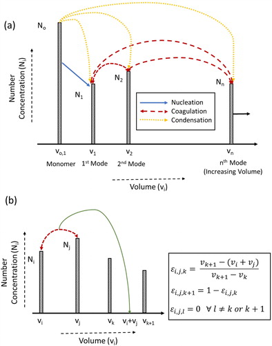
The nucleation, coagulation, and surface growth of particles are accounted for in this modal model and the developed model is generalized to incorporate “n” modes. Thus, the GDE (Equation (1)(1) $$\frac{\partial n\left(v,t\right)}{\partial t}+\nabla ·n\left(v,t\right)\mathit{u}+\frac{\partial \left(Gn\right)}{\partial v}-I\left(v^{\mathrm{*}}\right)\delta \left(v-v^{\mathrm{*}}\right)=\frac{1}{2}{\int }_0^v\beta \left(v-\tilde{v},v\right)n\left(v-\tilde{v},t\right)n\left(\tilde{v},t\right)d\tilde{v}-n\left(v,t\right){\int }_0^{\mathrm{\infty }}\beta \left(\tilde{v},v\right)n\left(\tilde{v},t\right)d\tilde{v}.$$(1) ) is equivalently solved by obtaining $N_k$ and $V_k$ as below: (4) $$\frac{d{N}_k}{dt}={\frac{d{N}_k}{dt}}_{\mathit{coag}}+{\frac{d{N}_k}{dt}}_{\mathit{nucl}},$$(4) (5) $$\frac{d{V}_k}{dt}={\frac{d{V}_k}{dt}}_{\mathit{coag}}+{\frac{d{V}_k}{dt}}_{\mathit{cond}/\mathit{evap}},$$(5) where $N_k$ is the number concentration of particles and $V_k$ is the total particle volume corresponding to $k\mathrm{th}$ mode for $1\le k\le n.$ The change of both $N_k$ and $V_k$ is shown in Appendix A4.

2.2. Coagulation

Coagulation is the collision of two particles, the result of which is larger than the stable critical size of the original particles. In this work, the Brownian coagulation coefficient is given by the Fuchs form of the coagulation coefficient (Seinfeld and Pandis 2016) for the discrete, discrete sectional, and modal models, whereas the method of moments used the expression in the work of Pratsinis (1988): (6) $${\beta }_{i,j}=2\pi \left(D_i+D_j\right)\left(d_i+d_j\right){\left(\frac{d_i+d_j}{d_i+d_j+2{\left({g_i}^2+{g_j}^2\right)}^{\frac{1}{2}}}+\frac{8\left(D_i+D_j\right)}{{\left({{\overline{c}}_i}^2+{{\overline{c}}_j}^2\right)}^{\frac{1}{2}}\left(d_i+d_j\right)}\right)}^{-1},\mathrm{ }$$(6) where the particle diffusion coefficient $D_i,$ particle velocity ${\overline{c}}_i,$ and transition parameter $g_i$ are given by: (7) $$D_i=\frac{k_{B}T{C}_C}{3\pi \mu d_i},\mathrm{ }{\overline{c}}_i={\left(\frac{8k_{B}T}{\pi m_i}\right)}^{\frac{1}{2}},\mathrm{ }{g}_i=\frac{\sqrt{2}}{3d_i{l}_i}\left({\left(d_i+l_i\right)}^3+{\left({d_i}^2+{l_i}^2\right)}^{3/2}\right)-d_i,$$(7) with the modified mean free path $l_i$ defined as: (8) $$l_i=\mathrm{ }\frac{8D_i}{\pi {\overline{c}}_i},$$(8)

Here, $d_i$ is the particle diameter, $k_B$ is the Boltzmann’s Constant, $T$ is the temperature, $C_C$ is the Cunningham slip correction factor and $m_i$ is the particle mass.

2.3. Nucleation

A stable cluster of molecules suspended in a medium defines the gas to particle conversion in a supersaturated vapor environment. There are several theories to explain this particle formation mechanism with classical homogeneous nucleation theory. I represents the nucleation rate, and is given by Friedlander (2000): (9) $$I=2\left[\frac{p_1}{{\left(2\pi m_1{k}_{B}T\right)}^{1/2}}\right]{\left(n_1{v}_1^{2/3}\right)\left[\frac{\sigma v_1^{2/3}}{k_{B}T}\right]}^{1/2}\mathrm{e}\mathrm{xp}\left[-\left(\frac{16\pi {\sigma }_{\mathrm{ }}^3{v}_1^2}{{3\left(k_{B}T\right)}^3{\left(\ln S\right)}^2}\right)\mathrm{ }\right],$$(9) where $p_1$ is the partial pressure of the vapor, $n_1$ is the number concentration of the vapor, ${\sigma }_{ }$ is the surface tension, and $S$ is the saturation ratio.

2.4. Condensation

In this study, the condensation growth law, $dv/dt$ is given by the Fuchs-Sutugin formula for the discrete, discrete sectional, and modal models (Fuchs and Sutugin 1971), whereas the harmonic mean of condensation coefficient for the free-molecular and continuum regime is used for the method of moments (seeing in Appendix B). Both the approaches are found to agree well with each other for all particle sizes (Pratsinis 1988): (10) $$\frac{dv}{dt}=\frac{2\pi d_p{D}_f{v}_1\left[P-P_s\mathrm{e}\mathrm{xp}\left(\frac{4\sigma v_1}{d_p{k}_{B}T}\right)\right]}{1+\left(\frac{1.333Kn+0.71}{1+Kn}\right)Kn},$$(10) where $d_p$ is the aerosol radius, $D_f$ is the diffusion coefficient of the condensing vapor, $Kn$ is the Knudsen number equal to $2\lambda /d_p,$ $\lambda$ is the mean free path of the condensing vapor, $v_1$ is the mass of the vapor molecule (or monomer)mass of the vapor molecule (or monomer), $n_1$ is the number concentration of the vapor, ${\sigma }_{ }$ is the surface tension, $k_B$ is the Boltzmann constant, $T$ is the temperature, and $S$ is the saturation ratio.

2.5. Coupling with COMSOL

The fluid flow and temperature profile in the furnace aerosol reactor is simulated as an application of AAQRL-ADM. This is performed by solving the Navier-Stokes equation for steady-state fluid flow. The velocity and temperature profile thus obtained can be used as an input file to the aerosol dynamic models.

2.6. Effects not considered

Several aerosol dynamics effects, such as diffusion loss, coagulation due to external forces or shear stress, thermophoretic loss, charged particle interactions, particle composition, evaporation of particles, reactive systems, fractal particles, and dense particle systems, are outside the scope of this software. However, the software is organized in modular form, and therefore can be easily modified to include some of these effects.

3. Software working principle

The working principle and the GUI design of AAQRL-ADM are shown in Figures 2 and 3. The input parameters are basic species and gas properties. As described in Section 2.2, nucleation, condensation and coagulation mechanisms can be selected as per the choice of the user. Furthermore, the software can import the simulation results of fluid flow and heat transfer from COMSOL and integrate with the aerosol dynamics solvers. The software output contains parameters such as the simulated PSD, saturation ratio of vapor (S), the total number concentration ($N_{\mathit{tot}}$), the total volume concentration ($V_{\mathit{tot}}$), the geometric mean diameter ($d_{pg}$), and the geometric mean standard deviation (${\sigma }_g$).

Figure 2. Working principle of AAQRL-ADM software.

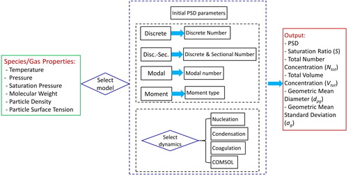
Figure 3. Graphical User Interface (GUI) of AAQRL-ADM (https://github.com/AAQRL/aerosol_dynamic_models; DOI: 10.5281/zenodo.3571284) software. (a) Main window; (b) Discrete model window.

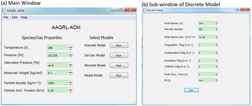
Figure 3 shows the GUI design of AAQRL-ADM software. After inputting the basic parameters of species and gas, four aerosol dynamic models can be chosen by clicking the “Run” button as shown in Figure 3a. Then a sub-window appears to show the model that the user selected. Users can input the parameters required in the corresponding model through this GUI. Figure 3b performs the example GUI of discrete model. The user guide of AAQRL-ADM is described in Appendix C.

4. Results and discussion

This section contains three parts: model validation, numerical efficiency of the different models and application. In the model validation part, four cases that include the effects of coagulation, condensation and nucleation are presented. The comparison of numerical efficiency of different models gives a guide to choosing models based on the discussion of the tradeoff between computational cost and simulation accuracy. Finally, the application for predicting the aerosol dynamics in a tubular furnace (Lin et al. 2018) is demonstrated. In this case, the gas velocity and temperature are coupled with the aerosol dynamic models. The discrete and discrete-sectional models are verified in the work of Biswas et al. (1997), Chadha et al. (2017), and Gao et al. (2017). The moment and modal models are verified in the work of Sharma, Wang, et al. (2019) and Zhang et al. (2018), and Wang et al. (2017), respectively.

4.1. Model validation

4.1.1. Pure coagulation

In this case, the ambient gas is assumed to be air (gas molecular weight = 29 g/mol), and the temperature and pressure are set to 300 K and 1 atm, respectively, with a total simulation time of 1 s. The initial PSD is assumed to be monodisperse with a diameter of 1 nm and a particle number concentration of 10¹⁰ cm⁻³. For the discrete model, 100 discrete sizes are chosen, for the modal model, 8 modes are used, and for the discrete-sectional model, 100 discrete sizes, and 119 sections are used. Only the effect of coagulation is considered here.

Figure 4a shows the PSD at the final simulation time by all four models. It can be seen that n(d_p) is approaching zero when d_p is near 4.5 nm. Theoretically, the simulation result by the discrete model is the most accurate compared with the other three models. So, the PSD calculated from the discrete model could be thought of as the benchmark result. It can be also seen from Figure 4a that the changing trend of PSD is the same for all models. In particular, n(d_p) predicted by the discrete and discrete-sectional models collapses into the same curve. For the modal, discrete, and discrete-sectional models, a peak in the PSD occurs at d_p ∼ 1.25 nm. We observe a sharp peak in the modal model, but the simulation result by the moment model is quite smooth, since the PSD is always assumed to be the lognormal form. Additionally, the statistical parameters of the different models are seen in Table 3a. Because of coagulation, N_tot drops from 10¹⁰ cm⁻³ to 2.04 × 10⁹ cm⁻³. d_pg lies in a narrow range from 1.46 nm (modal model) to 1.52 nm (moment model). σ_g is around 1.34 and agrees very well for all models.

Figure 4. The particle size distribution (PSD) after the final time for (a) monodisperse case and (b) lognormal case.

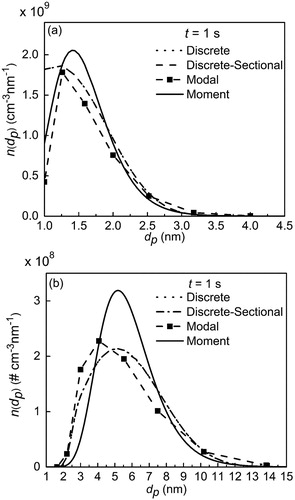
Table 3. Comparison of ensemble parameters by different models.

(a) Monodisperse
Parameters	Initial (monodisperse)	Discrete	Discrete-sectional	Modal	Moment
Ntot (#/cm^3)	1 × 10^10	2.04 × 10^9	2.04 × 10^9	2.04 × 10^9	2.04 × 10^9
dpg (nm)	1	1.49	1.49	1.46	1.52
σg	1	1.34	1.34	1.35	1.31
(b) Lognormal
Parameters	Initial (log-normal)	Discrete	Discrete-sectional	Modal	Moment
Ntot (#/cm^3)	1 × 10^10	1.13 × 10^9	1.14 × 10^9	1.13 × 10^9	1.23 × 10^9
dpg (nm)	3	5.50	5.51	5.23	5.62
σg	1.2	1.43	1.43	1.47	1.33

Next, the initial PSD is changed from monodisperse to lognormal distribution whose geometric mean diameter (d_pg) and standard deviation (σ_g) are 3 nm and 1.2, respectively. In the modal model for the lognormal case, 9 modes are used. In the discrete-sectional model, 300 discrete sizes and 195 sections are used. The discrete sizes are 20,000.

Figure 4b shows the simulation results of the PSD at t = 1 s by different models. The peak of the PSD appears around 5 nm (Figure 4b). The simulated PSDs by the discrete and discrete-sectional model agree very well. The result of the modal model also has a good match with the PSD by the discrete and discrete-sectional models, but for the moment model, the peak of the PSD is slightly overestimated.

Table 3b gives the statistical parameters at final simulation time for all four models. The discrete, discrete-sectional and modal models obtain almost the same value of N_tot, while the value by the moment model is a little higher than those for the other three models. Furthermore, all d_pg is between 5.23 and 5.62 nm. σ_g for the moment model is the smallest one and occurs because we assumed the log-normal form in the moment model, which predicts a narrower size distribution than in the discrete or discrete-sectional models (Otto et al. 1994, 1999).

4.1.2. Nucleation and coagulation

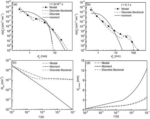
The effects of both nucleation and coagulation are considered for comparing the simulation results by all four models. The ambient temperature, vapor saturation pressure, vapor molecular weight, vapor density, and vapor surface tension are 1400 K, 10⁻³Pa, 79.8 g mol⁻¹, 4.23 g cm⁻³, and 25 × 10⁻³ N m⁻¹, respectively. The first particle size is set as the dimer with an initial number concentration of 3 × 10¹⁴ cm⁻³.

Figure 5 shows the simulation results of the discrete, discrete-sectional, moment and modal models. Due to the high computational burden, the simulations for the discrete model are performed only until t = 2 × 10⁻³ s. As seen in Figure 5a, the PSDs obtained by the discrete and discrete-sectional are almost indistinguishable from each other. Both models predict a bimodal particle size distribution, which is not computed by either the modal or moment models. As time progresses, shown in Figure 5b, the first nucleation peak continues at the first particle size, due to continuous influx of particles, whereas the coagulation peak shifts to the right for both the discrete-sectional and modal models. This figure also shows the inability of the moment model to capture the evolution of bimodal size distribution due to inherent assumption of lognormal distribution. This drawback can also be observed when the total number concentration, N_tot (Figure 5c) and the average particle diameter, d_p,mean = ${\left(\frac{6V_{\mathit{tot}}}{\pi N_{\mathit{tot}}}\right)}^{1/3}$ (Figure 5b) are compared between the different models as a function of time. The lognormal distribution assumption bounds the moment model, and it predicts significantly higher rates of coagulation than the other two models, which seem to agree well with each other.

Figure 5. Comparison of discrete, discrete-sectional, moment and modal modes when considering both coagulation and nucleation effects (a) simulated PSD at t = 2 × 10⁻³ s, (b) simulated PSD at t = 0.1 s, (c) total number concentration (N_tot) vs. time, and (d) mean diameter (d_p,mean) vs. time.

4.1.3. Condensation

In this part, the condensation modules of the discrete-sectional, modal and moment models are compared. The initial PSD is assumed to be lognormal with a d_pg of 10 nm and a σ_g of 1.5, and a total number concentration of 10⁵ cm⁻³. The initial vapor saturation was assumed to be 100 at the temperature of 390 K. The vapor molecular weight is 100 g mol⁻¹ and the vapor density is 1 g cm⁻³. Thus, the molecular diameter is 0.68 nm.

For the simulated time of 100 s, two cases (1) depleting vapor concentration, and (2) constant vapor concentration are considered. In the modal model, 8 modes are set. In the discrete-sectional model, 300 discrete sizes and 195 sections are set. Assuming the particle size ranges from 1 to 100 nm, the number required to present the entire PSD for the discrete model is approximately 3.2 × 10⁶, which carries a very high computational demand.¹

The results for the three models are compared. As the vapor continuously condenses on the particles, the PSD is expected to become close to monodisperse. The final size distributions of particles as predicted by the models are compared in Figure 6 for depleting and constant vapor concentration cases. The discrete-sectional model predicted more condensational growth and wider PSD for the constant vapor concentration case. Because the mode of the modal model could adjust its value with time in this work, the PSD by the modal model tends to concentrate at a certain d_p.

Figure 6. PSD vs. particle size for condensation case (a) depleting vapor concentration (b) constant vapor concentration.

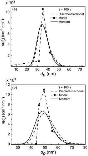
Furthermore, as can be seen from Table 4, the average parameters for the different models agree well at final simulation time. Because the vapor concentration is changing with time, the d_pg values in Table 4a are smaller than those in Table 4b. For constant vapor concentration, the PSD is found to be concentrated around d_pg, with a smaller spread than that for the depleting vapor scenario. This further validates our model to simulate condensation well, because in strictly condensational growth, particles tend to become monodisperse after a long time (Friedlander 2000).

Table 4. Comparison of ensemble parameters for particle condensation.

(a) Depleting vapor concentration.
Parameters	Discrete-sectional	Modal	Moment
Ntot (#/cm^3)	1.00 × 10^5	1.00 × 10^5	1.00 × 10^5
dpg (nm)	35.9	34.4	35.0
σg	1.16	1.37	1.16
(b) Constant vapor concentration
Parameters	Discrete-sectional	Modal	Moment
Ntot (#/cm^3)	1.00 × 10^5	1.00 × 10^5	1.00 × 10^5
dpg (nm)	50.9	50.0	49.0
σg	1.14	1.09	1.13

4.1.4. Nucleation, condensation and coagulation

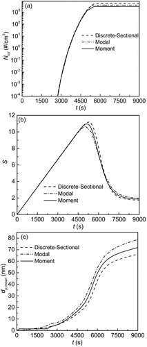
The combined effect of nucleation, condensation and coagulation on PSD is studied by the three models: discrete-sectional, modal and moment models. The vapor concentration is assumed to be zero at t = 0 s, with a constant rate of vapor generation of 5.4 × 10⁵ cm⁻³ s⁻¹. The vapor saturation pressure is kept constant at 10⁻⁶Pa at the temperature of 298 K. The vapor molecular weight, the vapor molecular density and the vapor surface tension are assumed to be 100 g mol⁻¹, 1 g cm⁻³, and 25 × 10⁻³ N m⁻¹, respectively. And there are no particles existing at the initial time. First, vapors nucleate to form the particles, which grow through condensation and coagulation. The nucleation rate is expressed in Equation (9)(9) $$I=2\left[\frac{p_1}{{\left(2\pi m_1{k}_{B}T\right)}^{1/2}}\right]{\left(n_1{v}_1^{2/3}\right)\left[\frac{\sigma v_1^{2/3}}{k_{B}T}\right]}^{1/2}\mathrm{e}\mathrm{xp}\left[-\left(\frac{16\pi {\sigma }_{\mathrm{ }}^3{v}_1^2}{{3\left(k_{B}T\right)}^3{\left(\ln S\right)}^2}\right)\mathrm{ }\right],$$(9) . Nine modes are used in the modal model. For the discrete-sectional model, 30 discrete sizes and 252 sections are used, while the first discrete size is set as the vapor phase (or monomer), and the dimer is set as the first particle size. In this case, a long simulation time of 9000 s is used.

Figure 7a shows the total number concentration (N_tot) vs. simulation time (t). N_tot grows rapidly to a magnitude that is of the order of 10³ cm⁻³ and becomes almost constant. Figure 7b shows the linear increase in vapor concentration as time progresses. When t is beyond 4500 s, S begins to decrease because the nucleation rate reaches ∼10⁶ cm⁻³ s⁻¹. As time progresses, vapor consumption is dominated by condensation rather than nucleation. Figure 7c shows the mean diameter d_p,meam vs. t. The simulated d_p,mean is also close in both magnitude and trend with time for all three models.

Figure 7. Simulation results of simultaneous nucleation, condensation and coagulation case (a) N_tot vs. t, (b) saturation ratio (S) vs. t, and (c) mean diameter (d_p,mean) vs. t.

4.2. Numerical efficiency

The test of numerical efficiency of all four models is performed using the facilities of the Washington University Center for High Performance Computing (CHPC). The CPU that CHPC uses is the Intel 8-core Xeon E5-2630v3 (2133 MHz). Table 5 gives the computational time costs by each model for the different cases. For the pure coagulation case with initial monodisperse PSD (seeing the case condition in Section 4.4.1), the computational time costs for all models are less than 30 s. However, for the pure coagulation case with an initial PSD of lognormal distribution, the computation time cost of the discrete model reaches over 35 h as compared to 105.00 s, 16.00 s, and 0.066 s for the discrete-sectional, modal, and moment models. The reason that the discrete model takes a relatively large value of computational time is the large number of discrete sizes (20,000) needed to obtain a converged simulation result (shown in Figure 8). In this figure, the computational time cost of the discrete model is demonstrated to be proportional to $N_{\mathit{dis}}^2.$ Thus, the discrete model is not realistic to simulate when large $N_{\mathit{dis}}$ is needed to obtain the convergence simulation result. The relationship between the metric of judging whether the simulation result is converged (V_tot is considered as the metric) and the model parameters of the discrete-sectional and modal models is shown in Figures S1 and S2 in the online supplemental information.

Figure 8. Computational time and V_tot vs. discrete number for pure coagulation case with initial PSD of lognormal distribution. (open square: V_tot; closed square: CPU time cost; dash line: fitting curve for CPU time cost).

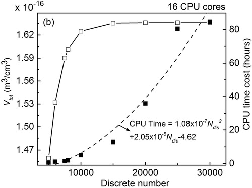
Table 5. Comparison of computational time cost of different models.

Models	Pure coagulation case with monodisperse initial PSD
	Model parameters	Computational time cost (s)	Computer property
Discrete	Discrete number: 100	5.30 × 10^–1	1 CPU core
Discrete-sectional	Discrete number: 100, Sectional number: 119	1.17 × 10^1	1 CPU core
Modal	Model number: 8	2.60 × 10^1	1 CPU core
Moment	–	5.2 × 10^–2	1 CPU core
Models	Pure coagulation case with lognormal initial PSD
	Model parameters	Computational time cost (s)	Computer property
Discrete	Discrete number: 20,000	1.29 × 10^5	16 CPU cores
Discrete-sectional	Discrete number: 300, Sectional number:119	1.05 × 10^2	1 CPU core
Modal	Model number:8	1.60 × 10^1	1 CPU core
Moment	–	6.6 × 10^–2
Models	Nucleation and coagulation
	Model parameters	Computational time cost (s)	Computer property
Discrete	Discrete number: 8000	1.29 × 10^4	8 CPU cores
Discrete-sectional	Discrete number: 200, Sectional number: 263	1.20 × 10^3	1 CPU core
Modal	Model number: 12	4.65 × 10^2	1 CPU core
Moment	–	5.13 × 10^0	1 CPU core

For the case of nucleation and coagulation, the simulation time is set at 2 × 10⁻³ s. Even for such small simulation time, the CPU time cost for the discrete model reaches to 8.72 h, which is much higher than that of the discrete-sectional, modal, and moment models. However, as discussed earlier, the moment model is unable to capture the bimodal aspect of the PSD and predicts significantly higher coagulation, as shown in Figures 5a and b.

From this section, we find that the moment model is least computationally expensive but also reasonably accurate for the coagulation-only case. This is because in the case of coagulation, the size distribution eventually becomes a self-preserving PSD which can be approximated as lognormal (seeing Figure D1 in Appendix D). Thus, for the coagulation-only case, the moment model performs the best of the four models.

While the discrete model is accurate, it cannot obtain the results for longer simulation times. The discrete-sectional model is much more efficient than the discrete model, but due to the numerical diffusion and the impact on the accuracy by the discrete and sectional numbers, it is computationally more expensive than the moment and modal models. The modal model works best for this case as it is less computationally expensive than the discrete and discrete-sectional models and is able to capture the bimodal aspect of the PSD. Thus, if coagulation and condensation are the only dominant mechanisms, first the moment model should be used, whereas if nucleation is also taking place, then the modal model should be used in order to obtain a quick understanding of the evolution of the PSD with time. However, for high accuracy, the discrete-sectional model is suggested. On the other hand, the highly accurate discrete model can only be used with high computational cost, and is limited to the simulations of very early stages of particle formation, and growth (sub-10 nm particles) (Lehtinen and Kulmala 2003).

4.3. Application

In this section, the discrete-sectional, moment and modal models are used to study a practical case: investigation of the particle size distribution in a furnace aerosol reactor. Due to the high computational burden involved, the discrete model is not evaluated for this application. A single-step furnace aerosol reactor (FuAR) technique is widely used in synthesizing the catalysts, such as ZnO_1-x/C and TiO₂/NrGO, for CO₂ photoreduction (Lin et al. 2017, 2018). The precursor solution is nebulized into tiny droplets, which enter the furnace tube with a carrier gas. Usually, the droplets evaporate quickly after they enter the furnace tube (He et al. 2017) forming particles that are grown by coagulation.

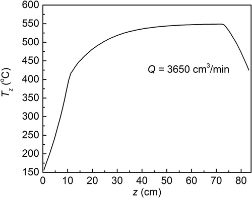
The aerosol reacting part of the FuAR is a tube that is shown in Figure 9a. The surface temperature of the tube (T₀) was kept constant. Assuming the flow of the carrier gas was axisymmetric in the furnace tube, the velocity and temperature were simulated in a simplified two-dimensional domain (Figure 9b) by a COMSOL 5.3a with a gas flow rate of Q = 3650 cm³/min, and a surface temperature of T₀ was 550 °C. Figure 10 shows the gas temperature profile along the z-axis. Since the tube inlet and outlet are connected to the atmosphere environment, the gas temperature rises gradually when it enters the inlet and begins to decrease near the tube outlet.

Figure 9. Schematic of (a) the furnace tube and (b) the computational domain (L = 83.5 cm; R = 0.95 cm).

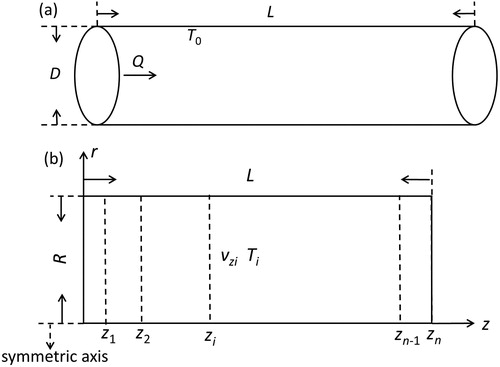
Figure 10. Gas temperature profile along z-axis in the furnace tube.

At the FuAR inlet, it was assumed that the initial PSD was monodisperse with an initial number concentration of 10¹⁰ cm⁻³ and a particle diameter of 20 nm. The discrete-sectional, moment and modal models were used to study the PSD along the z-axis. Ten modes were set in the modal model. In the discrete-sectional model, 50 discrete sizes and 108 sections were set.

Figure 11 compares the simulation results from the modal, moment and discrete-sectional models at different z-axes. In all three models, as the particles move from the inlet to the outlet, the distribution becomes wider, and the peak values of the PSD decrease due to coagulation, leading to the formation of larger particles. All three models compare well with each other, with some differences. Since the moment model is dependent on the free molecular expression of coagulation, the geometric standard deviation is expected to be close to 1.32 (Lee, Chen, and Gieseke 1984). The discrete-sectional model and modal model show a slightly higher value for geometric standard deviation due to the inclusion of sections and modes, respectively, which determine the spread of the distribution. The higher spread in the distribution promotes more collisional growth, and therefore the particles grow to larger sizes in the modal model than in the moment and discrete-sectional models. Table 6 gives the average parameters of PSD, N_tot, d_pg, and σ_g calculated by the three models at the different z-axes.

Figure 11. Comparison of simulated PSD by discrete-sectional, modal, and moment models at different positions.

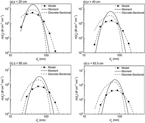
Table 6. Comparison of ensemble parameters by discrete-sectional, modal, and moment models for different positions.

(a) z = 20 cm
Parameters	Discrete-sectional	Modal	Moment
Ntot (#/cm^3)	3.34 × 10^8	2.86 × 10^8	5.93 × 10^8
dpg (nm)	44.1	49.6	46.2
σg	1.40	1.55	1.31
(b) z = 40 cm
Parameters	Discrete-sectional	Modal	Moment
Ntot (#/cm^3)	1.64 × 10^8	1.14 × 10^8	2.66 × 10^8
dpg (nm)	54.3	67.2	60.6
σg	1.39	1.56	1.31
(c) z = 60 cm
Parameters	Discrete-sectional	Modal	Moment
Ntot (#/cm^3)	1.12 × 10^8	6.69 × 10^7	1.70 × 10^8
dpg (nm)	61.4	80.2	70.5
σg	1.39	1.56	1.31
(d) z = 83.5 cm
Parameters	Discrete-sectional	Modal	Moment
Ntot (#/cm^3)	9.90 × 10^7	4.42 × 10^7	1.20 × 10^8
dpg (nm)	68.0	92.1	79.2
σg	1.38	1.56	1.30

5. Summary

Aerosol dynamics modeling is an important aspect of research in aerosol science and engineering. In this work, an open source software code with a graphical user interface (GUI), AAQRL-ADM, is developed to perform aerosol dynamics simulations. Four different aerosol dynamics models, the discrete, discrete-sectional, modal, and method of moments, are validated and simulated for different cases of coagulation, condensation, and nucleation. Moreover, these models are coupled with the velocity and temperature profiles obtained from the COMSOL.

The users of this software for research purposes are advised that for a first order estimation of the aerosol dynamics problem, a simple method of moments should be used if only coagulation, and condensation are the dominant mechanisms due to its low computational cost and reasonable accuracy. On the other hand, if nucleation is also considered, a modal model should be a good starting point, as it is not restricted by the lognormal assumption of the moment model. If more accuracy is required, the discrete-sectional model can also be used with the appropriate number of discrete sizes and sections. The discrete model, even though the most accurate model for the given conditions, is computationally very expensive, as the computational time for simulations is found to scale as $N_{\mathit{dis}}^2.$ Nevertheless, the discrete model still has applications in understanding early stages of particle formation and growth (sub-10 nm), both in atmospheric simulations and in aerosol reactors.

Nomenclature
dp	=	particle diameter, nm
dpg	=	geometric mean diameter, nm
dp,mean	=	mean diameter, nm
D	=	diameter of furnace tube, cm
$D_f$	=	diffusion coefficient of the condensing vapor, cm2/s
$D_v$	=	vapor diffusivity coefficient, m2 s−1
G	=	particle condensation rate, cm3 s−1
I	=	nucleation rate, cm−3 s−1
I’	=	dimensionless nucleation rate
J0	=	monomer generation rate, cm−3 s−1
$k_B$	=	Boltzmann constant, m2 kg s−2 K−1
k*	=	number of monomers in the critical size nucleus
$K_n$	=	Knudsen number
L	=	length of furnace tube, cm
n	=	particle size distribution function, cm−3 nm−1 or mode number
ni	=	particle number concentration of i-th discrete size, cm−3
$n_{\mathit{sat}}$	=	saturation number concentration of vapor (or monomer), cm−3
n1,sat	=	monomer concentration at saturation, cm−3
Ni	=	number concentration of particles of ith mode, cm−3
$N_{\mathit{dis}}$	=	total number of discrete sizes
Ntot	=	total number concentration of particles, cm−3
N’	=	dimensionless particle number concentration
$m_1$	=	mass of the vapor (or monomer) molecule, kg
M	=	moment of particle size distribution
p1	=	partial pressure of the vapor (or monomer), Pa
qi	=	particle population function of discrete size i
qi,sat	=	saturation particle population function on the surface of discrete size i
Q	=	gas flow rate, cm3 min−1
Qk	=	particle population function of section k
Qk,sat	=	saturation particle population function on the surface of section k
r	=	radius axis of furnace tube, cm
R	=	vapor generation rate, cm−3 s−1
R′	=	dimensionless vapor generation rate
s1	=	monomer surface area, cm2
S	=	saturation ratio
t	=	time, s
T	=	ambient temperature, K
T0	=	temperature on the wall of furnace tube, K
u	=	velocity of the carrier gas, m/s
v	=	particle volume, cm3
$\tilde{v}$	=	particle volume, cm3
v1	=	vapor molecular (or monomer) volume or the volume of the first discrete size, cm3
vg	=	geometric mean volume
vzi	=	gas velocity at different positions, cm
$v^{*}$	=	critical particle volume, cm3
$V_i$	=	total particle volume of ith mode
Vtot	=	total volume concentration, m3 cm−3
$\overline{V}$	=	dimensionless particle volume concentration
z	=	symmetric axis of furnace tube, cm

Greek letters
$\beta$	=	coagulation collision frequency function, cm3 s−1
${\beta }_{i,j}$	=	coagulation collision frequency function between i-mers and j-mers or i-mode and j-mode, cm3 s−1
$\overline{\beta }$	=	coagulation collision frequency function between sections, cm3 s−1
${\overline{\beta }}^D$	=	coagulation collision frequency function between discrete size and section, cm3 s−1
${\overline{\beta }}^{DD}$	=	coagulation collision frequency function between discrete sizes, cm3 s−1
${\overline{\beta }}^{\mathit{DDS}}$	=	coagulation collision frequency function between discrete sizes to form section, cm3 s−1
$\epsilon$	=	apportionment factor
$ϵ$	=	dimensionless coagulation coefficient
$\zeta$	=	population index: 0-number, 1-volume, 2-volume square
η	=	dimensionless condensation coefficient
$\theta$	=	a logical operator used in the integration of $\beta$
$\lambda$	=	mean free path of the condensing vapor, nm
ξ	=	dimensionless coagulation coefficient
$\sigma$	=	surface tension, N m−1
σg	=	geometric standard deviation
τ	=	characteristic time for particle growth, s
$\Theta$	=	dimensionless residence time

Subscript
C	=	continuum regime
FM	=	free molecular regime
i	=	i-mers or i-mode
j	=	j-mers or j-mode
k	=	k-mers or k-section or kth moment or k-mode
m	=	total number

Acknowledgments

The computing of the discrete and modal models was performed using the facilities of the Washington University Center for High Performance Computing (CHPC), which is partially funded by grant NCRR 1S10RR022984-01A1.

Funding

This work was supported by a grant from the National Science Foundation, SusChEM: Ultrafine Particle Formation in Advanced Low Carbon Combustion Processes; CBET 1705864. H.Z. was supported by the Natural Science Foundation of Beijing [Grant No. 3184051]. High Performance Computing (CHPC) is partially funded by grant NCRR 1S10RR022984-01A1.

Notes

1 As described in the introduction of the discrete model, the total number of discrete size needed in the condensation case is estimated as (100 nm/0.68 nm)³ ∼ 3.2 × 10⁶.

Appendix A

A1 Discrete model

In the discrete model, the continuous PSD, n(v), is discretized by discrete number concentration, $n_1,$ $n_2,$ $n_3,$ … $n_i,$ … and $n_l.$ The particle volume for the ith discrete size ($v_i$) equals $v_1+(i{-1)v}_m,$ where $v_1$ is the volume of the first discrete size and $v_m$ is the molecular volume. Note that n(v) in Equation (1)(1) $$\frac{\partial n\left(v,t\right)}{\partial t}+\nabla ·n\left(v,t\right)\mathit{u}+\frac{\partial \left(Gn\right)}{\partial v}-I\left(v^{\mathrm{*}}\right)\delta \left(v-v^{\mathrm{*}}\right)=\frac{1}{2}{\int }_0^v\beta \left(v-\tilde{v},v\right)n\left(v-\tilde{v},t\right)n\left(\tilde{v},t\right)d\tilde{v}-n\left(v,t\right){\int }_0^{\mathrm{\infty }}\beta \left(\tilde{v},v\right)n\left(\tilde{v},t\right)d\tilde{v}.$$(1) is the distribution function of number concentration, while $n_i$ for the discrete model represents the number concentration.

In the case of coagulation, the discrete model is shown as: (A1) $$\frac{\partial n_1}{\partial t}=-n_1\sum _{i=1}^l{\beta }_{1,i}{n}_i,$$(A1) (A2) $$\frac{\partial n_k}{\partial t}=\frac{1}{2}\sum _{i+j=k}^l{\beta }_{i,j}{n}_i{n}_j-n_k\sum _{i=1}^l{\beta }_{1,i}{n}_i.\mathrm{ }(k>1)$$(A2)

The discrete model that includes the effect of condensation and nucleation is discussed in the following section.

A2 Discrete-sectional model

Instead of representing every possible particle size, the discrete-sectional model uses sections to account for the integral property for large particles. Consider a certain particle with its size characterized by volume $v.$ The bulk particle size domain is divided into the discrete size regime (DSR) consisting of l discrete sizes and the sectional size regime (SSR) consisting of K sections.

Let $n_i(i{v}_1)$ represent the number concentration in the DSR, where $v_1$ represents the volume of the monomer. Furthermore, a general particle property can be introduced as: (A3) $$q_i=n_i\left(i{v}_1\right)·{\left(i{v}_1\right)}^{\zeta },$$(A3) where $\zeta$ is the particle property index such that, when $\zeta =0, q_i$ is the number concentration, and at $\zeta =1, q_i$ is the particle volume concentration. Moreover, if the particle size domain in the SSR is divided into $k$ arbitrary sections, an integral property can be defined as: (A4) $$Q_k={N_k}_{\mathrm{ }}\left(v_k\right)\mathrm{ }·{\left(v_k\right)}^{\zeta },\mathrm{ }$$(A4) where, $N_k\left(v_k\right)$ denotes the number concentration of section k. $v_1\left(l+\frac{1}{2}\right)$ is used to represent the starting size of SSR (Wu and Flagan 1988). The discrete-sectional model derives a general conservation equation for $q_i$ and $Q_k$ by accounting for the gain and loss of the aforementioned terms in the DSR and SSR due to the different particle phenomena such as nucleation, coagulation and condensation. Thus, the discrete-sectional model of single-component particle dynamics is shown as below: (A5) $$\frac{d{q}_2}{dt}=I-q_2\sum _{j=1}^{{\mathit{max}}_{\mathrm{ }}}{{{}_{\mathrm{ }}{}^2\overline{\beta }}_{2,j}^{DD}q}_j-q_2\sum _{k=1}^{\mathit{max}}{{}_{\mathrm{ }}{}^4\overline{\beta }}_{2,k}^D{Q}_k-{{}_{\mathrm{ }}{}^4\overline{\beta }}_{1,2}^{DD}\left(q_1-q_{2,\mathit{sat}}\right)q_2$$(A5) (A6) $$\frac{d{q}_i}{dt}=\frac{1}{2}\sum _{j=2}^{i-2}{{}_{\mathrm{ }}{}^1\overline{\beta }}_{j,i-j,i}^{DD}{q}_j{q}_{i-j}-q_i\sum _{j=2}^{{\mathit{max}}_{\mathrm{ }}}{{}_{\mathrm{ }}{}^2\overline{\beta }}_{i,j}^{DD}{q}_j-{q_i}_{\mathrm{ }}\sum _{k=1}^{\mathit{max}}{{}_{\mathrm{ }}{}^4\overline{\beta }}_{i,k}^D{Q}_k-{{}_{\mathrm{ }}{}^4\overline{\beta }}_{1,i}^{DD}\left(q_1-q_{i,\mathit{sat}}\right)q_i+{{}_{\mathrm{ }}{}^1\overline{\beta }}_{1,i-1,i}^{DD}\left(q_1-q_{i-1,\mathit{sat}}\right)q_{i-1}$$(A6) (A7) $$\frac{d{Q}_1}{dt}=\frac{1}{2}\sum _{i=2}^{\max \mathrm{ }}\sum _{j=2}^{{\mathit{max}}_{\mathrm{ }}}{{}_{\mathrm{ }}{}^1\overline{\beta }}_{i,j}^{DD}{q}_i{q}_j\mathrm{ }-Q_1\sum _{i=2}^{{\mathit{max}}_{\mathrm{ }}}{{}_{\mathrm{ }}{}^2\overline{\beta }}_{i,1}^D{q}_i+Q_1\sum _{i=2}^{{\mathit{max}}_{\mathrm{ }}}{{}_{\mathrm{ }}{}^5\overline{\beta }}_{i,1}^D{q}_i-\frac{1}{2}{{}_{\mathrm{ }}{}^3\overline{\beta }}_1^{\mathrm{ }}{Q_1}^2+\frac{1}{2}{{}_{\mathrm{ }}{}^6\overline{\beta }}_1^{\mathrm{ }}{Q_1}^2-Q_1\sum _{i=2}^{\mathit{max}}{{}_{\mathrm{ }}{}^4\overline{\beta }}_{1,i}^{\mathrm{ }}{Q}_i-{{{}_{\mathrm{ }}{}^2\overline{\beta }}_{1,1}^D\left(q_1-Q_{1,\mathit{sat}}\right)Q}_1+{{{}_{\mathrm{ }}{}^5\overline{\beta }}_{1,1}^D\left(q_1-Q_{1,\mathit{sat}}\right)Q}_1+{{}_{\mathrm{ }}{}^1\overline{\beta }}_{1,{\mathit{max}}_{},1}^{\mathit{DDS}}\left(q_1-q_{\mathit{max},\mathit{sat}}\right)q_{\mathit{max}}$$(A7) (A8) $$\frac{d{Q}_k}{dt}=\frac{1}{2}{\sum _{i=2}^{{\mathit{max}}_{\mathrm{ }}}{\sum _{j=2}^{{\mathit{max}}_{\mathrm{ }}}\mathrm{ }{}_{}{}^1\overline{\beta }}_{i,j,k}^{\mathit{DDS}}q}_i{q}_j-\sum _{i=2}^{{\mathit{max}}_{}}{\sum _{j=2}^{k-1}{}_{}{}^1\overline{\beta }}_{i,j,k}^D{q}_i{Q}_j+\frac{1}{2}\sum _{i=1}^{k-1}\sum _{j=1}^{k-1}{{}_{}{}^1\overline{\beta }}_{i,j,k}^D{Q}_i{Q}_j+Q_k\sum _{i=2}^{{\mathit{max}}_{}}{{}_{}{}^2\overline{\beta }}_{i,k}^D{q}_i-{Q_k\sum _{i=1}^{k-1}{{}_{}{}^2\overline{\beta }}_{i,k}^{}{Q}_i+}_{}{Q}_k\sum _{i=2}^{{\mathit{max}}_{}}{{}_{}{}^5\overline{\beta }}_{i,k}^D{q}_i+Q_k\sum _{i=1}^{k-1}{{}_{}{}^5\overline{\beta }}_{i,k}^{}{Q}_i+-\frac{1}{2}{{}_{}{}^3\overline{\beta }}_k^{}{Q_k}^2+\frac{1}{2}{{}_{}{}^6\overline{\beta }}_k^{}{Q_k}^2-{Q_k\sum _{i=k+1}^{\mathit{max}}{{}_{}{}^2\overline{\beta }}_{i,k}^{}{Q}_i-}_{}{{}_{}{}^2\overline{\beta }}_{1,k}^D{\left(q_1-Q_{k,\mathit{sat}}\right)Q}_k+{{}_{}{}^5\overline{\beta }}_{1,k}^D{\left(q_1-Q_{k,\mathit{sat}}\right)Q}_k+{{}_{}{}^1\overline{\beta }}_{1,k-1}^D{\left(q_1-Q_{k-1,\mathit{sat}}\right)Q}_{k-1}$$(A8)

Note that Equation (A5(A5) $$\frac{d{q}_2}{dt}=I-q_2\sum _{j=1}^{{\mathit{max}}_{\mathrm{ }}}{{{}_{\mathrm{ }}{}^2\overline{\beta }}_{2,j}^{DD}q}_j-q_2\sum _{k=1}^{\mathit{max}}{{}_{\mathrm{ }}{}^4\overline{\beta }}_{2,k}^D{Q}_k-{{}_{\mathrm{ }}{}^4\overline{\beta }}_{1,2}^{DD}\left(q_1-q_{2,\mathit{sat}}\right)q_2$$(A5) ) is the conservation equation for the dimer (first particle) as $q_1$ is the property function of the vapor phase (monomer). Equation (A6(A6) $$\frac{d{q}_i}{dt}=\frac{1}{2}\sum _{j=2}^{i-2}{{}_{\mathrm{ }}{}^1\overline{\beta }}_{j,i-j,i}^{DD}{q}_j{q}_{i-j}-q_i\sum _{j=2}^{{\mathit{max}}_{\mathrm{ }}}{{}_{\mathrm{ }}{}^2\overline{\beta }}_{i,j}^{DD}{q}_j-{q_i}_{\mathrm{ }}\sum _{k=1}^{\mathit{max}}{{}_{\mathrm{ }}{}^4\overline{\beta }}_{i,k}^D{Q}_k-{{}_{\mathrm{ }}{}^4\overline{\beta }}_{1,i}^{DD}\left(q_1-q_{i,\mathit{sat}}\right)q_i+{{}_{\mathrm{ }}{}^1\overline{\beta }}_{1,i-1,i}^{DD}\left(q_1-q_{i-1,\mathit{sat}}\right)q_{i-1}$$(A6) ) corresponds to the other $q_i$ (i > 2), while Equations (A7)(A7) $$\frac{d{Q}_1}{dt}=\frac{1}{2}\sum _{i=2}^{\max \mathrm{ }}\sum _{j=2}^{{\mathit{max}}_{\mathrm{ }}}{{}_{\mathrm{ }}{}^1\overline{\beta }}_{i,j}^{DD}{q}_i{q}_j\mathrm{ }-Q_1\sum _{i=2}^{{\mathit{max}}_{\mathrm{ }}}{{}_{\mathrm{ }}{}^2\overline{\beta }}_{i,1}^D{q}_i+Q_1\sum _{i=2}^{{\mathit{max}}_{\mathrm{ }}}{{}_{\mathrm{ }}{}^5\overline{\beta }}_{i,1}^D{q}_i-\frac{1}{2}{{}_{\mathrm{ }}{}^3\overline{\beta }}_1^{\mathrm{ }}{Q_1}^2+\frac{1}{2}{{}_{\mathrm{ }}{}^6\overline{\beta }}_1^{\mathrm{ }}{Q_1}^2-Q_1\sum _{i=2}^{\mathit{max}}{{}_{\mathrm{ }}{}^4\overline{\beta }}_{1,i}^{\mathrm{ }}{Q}_i-{{{}_{\mathrm{ }}{}^2\overline{\beta }}_{1,1}^D\left(q_1-Q_{1,\mathit{sat}}\right)Q}_1+{{{}_{\mathrm{ }}{}^5\overline{\beta }}_{1,1}^D\left(q_1-Q_{1,\mathit{sat}}\right)Q}_1+{{}_{\mathrm{ }}{}^1\overline{\beta }}_{1,{\mathit{max}}_{},1}^{\mathit{DDS}}\left(q_1-q_{\mathit{max},\mathit{sat}}\right)q_{\mathit{max}}$$(A7) and (A8)(A8) $$\frac{d{Q}_k}{dt}=\frac{1}{2}{\sum _{i=2}^{{\mathit{max}}_{\mathrm{ }}}{\sum _{j=2}^{{\mathit{max}}_{\mathrm{ }}}\mathrm{ }{}_{}{}^1\overline{\beta }}_{i,j,k}^{\mathit{DDS}}q}_i{q}_j-\sum _{i=2}^{{\mathit{max}}_{}}{\sum _{j=2}^{k-1}{}_{}{}^1\overline{\beta }}_{i,j,k}^D{q}_i{Q}_j+\frac{1}{2}\sum _{i=1}^{k-1}\sum _{j=1}^{k-1}{{}_{}{}^1\overline{\beta }}_{i,j,k}^D{Q}_i{Q}_j+Q_k\sum _{i=2}^{{\mathit{max}}_{}}{{}_{}{}^2\overline{\beta }}_{i,k}^D{q}_i-{Q_k\sum _{i=1}^{k-1}{{}_{}{}^2\overline{\beta }}_{i,k}^{}{Q}_i+}_{}{Q}_k\sum _{i=2}^{{\mathit{max}}_{}}{{}_{}{}^5\overline{\beta }}_{i,k}^D{q}_i+Q_k\sum _{i=1}^{k-1}{{}_{}{}^5\overline{\beta }}_{i,k}^{}{Q}_i+-\frac{1}{2}{{}_{}{}^3\overline{\beta }}_k^{}{Q_k}^2+\frac{1}{2}{{}_{}{}^6\overline{\beta }}_k^{}{Q_k}^2-{Q_k\sum _{i=k+1}^{\mathit{max}}{{}_{}{}^2\overline{\beta }}_{i,k}^{}{Q}_i-}_{}{{}_{}{}^2\overline{\beta }}_{1,k}^D{\left(q_1-Q_{k,\mathit{sat}}\right)Q}_k+{{}_{}{}^5\overline{\beta }}_{1,k}^D{\left(q_1-Q_{k,\mathit{sat}}\right)Q}_k+{{}_{}{}^1\overline{\beta }}_{1,k-1}^D{\left(q_1-Q_{k-1,\mathit{sat}}\right)Q}_{k-1}$$(A8) are the conservation equations for the first section and other sections, respectively. I represents the nucleation rate at which the property of the first particle size ($q_2$) is formed from the vapor (monomer) and is defined in Equation (9)(9) $$I=2\left[\frac{p_1}{{\left(2\pi m_1{k}_{B}T\right)}^{1/2}}\right]{\left(n_1{v}_1^{2/3}\right)\left[\frac{\sigma v_1^{2/3}}{k_{B}T}\right]}^{1/2}\mathrm{e}\mathrm{xp}\left[-\left(\frac{16\pi {\sigma }_{\mathrm{ }}^3{v}_1^2}{{3\left(k_{B}T\right)}^3{\left(\ln S\right)}^2}\right)\mathrm{ }\right],$$(9) . If the vapor is considered to be depleted with time, the conservation equation for the vapor molecule (or monomer) is given as: (A9) $$\frac{d{q}_1}{dt}=-I-\sum _{j=1}^{\mathit{max}}{{}_{}{}^2\overline{\beta }}_{1,j}^{DD}\left(q_1-q_{j,\mathit{sat}}\right)q_j-\sum _{k=1}^{\mathit{max}}{{}_{}{}^4\overline{\beta }}_{1,k}^{DD}\left(q_1-Q_{k,\mathit{sat}}\right)Q_k.$$(A9)

Furthermore, the second term on the RHS of Equation (A5(A5) $$\frac{d{q}_2}{dt}=I-q_2\sum _{j=1}^{{\mathit{max}}_{\mathrm{ }}}{{{}_{\mathrm{ }}{}^2\overline{\beta }}_{2,j}^{DD}q}_j-q_2\sum _{k=1}^{\mathit{max}}{{}_{\mathrm{ }}{}^4\overline{\beta }}_{2,k}^D{Q}_k-{{}_{\mathrm{ }}{}^4\overline{\beta }}_{1,2}^{DD}\left(q_1-q_{2,\mathit{sat}}\right)q_2$$(A5) ) represents the loss of dimers due to coagulation with particles in the DSR, and the third term represents the loss due to coagulation with the particles in the SSR. The fourth term represents the loss due to condensation, in which $q_{2,\mathit{sat}}$ is the saturation particle population function at the surface of the second discrete size and is given by: (A10) $$q_{i,\mathit{sat}}=\left[n_{\mathit{sat}}\mathrm{e}\mathrm{xp}\left(\frac{4{\sigma }_{}{v}_1}{d_{p,i}{k}_{B}T}\right)\right]{v_1}^{\zeta },$$(A10) where the terms in the exponential expression account for the Kelvin effect.

Similarly, the terms in the RHS of Equations (A6)(A6) $$\frac{d{q}_i}{dt}=\frac{1}{2}\sum _{j=2}^{i-2}{{}_{\mathrm{ }}{}^1\overline{\beta }}_{j,i-j,i}^{DD}{q}_j{q}_{i-j}-q_i\sum _{j=2}^{{\mathit{max}}_{\mathrm{ }}}{{}_{\mathrm{ }}{}^2\overline{\beta }}_{i,j}^{DD}{q}_j-{q_i}_{\mathrm{ }}\sum _{k=1}^{\mathit{max}}{{}_{\mathrm{ }}{}^4\overline{\beta }}_{i,k}^D{Q}_k-{{}_{\mathrm{ }}{}^4\overline{\beta }}_{1,i}^{DD}\left(q_1-q_{i,\mathit{sat}}\right)q_i+{{}_{\mathrm{ }}{}^1\overline{\beta }}_{1,i-1,i}^{DD}\left(q_1-q_{i-1,\mathit{sat}}\right)q_{i-1}$$(A6) to (A8)(A8) $$\frac{d{Q}_k}{dt}=\frac{1}{2}{\sum _{i=2}^{{\mathit{max}}_{\mathrm{ }}}{\sum _{j=2}^{{\mathit{max}}_{\mathrm{ }}}\mathrm{ }{}_{}{}^1\overline{\beta }}_{i,j,k}^{\mathit{DDS}}q}_i{q}_j-\sum _{i=2}^{{\mathit{max}}_{}}{\sum _{j=2}^{k-1}{}_{}{}^1\overline{\beta }}_{i,j,k}^D{q}_i{Q}_j+\frac{1}{2}\sum _{i=1}^{k-1}\sum _{j=1}^{k-1}{{}_{}{}^1\overline{\beta }}_{i,j,k}^D{Q}_i{Q}_j+Q_k\sum _{i=2}^{{\mathit{max}}_{}}{{}_{}{}^2\overline{\beta }}_{i,k}^D{q}_i-{Q_k\sum _{i=1}^{k-1}{{}_{}{}^2\overline{\beta }}_{i,k}^{}{Q}_i+}_{}{Q}_k\sum _{i=2}^{{\mathit{max}}_{}}{{}_{}{}^5\overline{\beta }}_{i,k}^D{q}_i+Q_k\sum _{i=1}^{k-1}{{}_{}{}^5\overline{\beta }}_{i,k}^{}{Q}_i+-\frac{1}{2}{{}_{}{}^3\overline{\beta }}_k^{}{Q_k}^2+\frac{1}{2}{{}_{}{}^6\overline{\beta }}_k^{}{Q_k}^2-{Q_k\sum _{i=k+1}^{\mathit{max}}{{}_{}{}^2\overline{\beta }}_{i,k}^{}{Q}_i-}_{}{{}_{}{}^2\overline{\beta }}_{1,k}^D{\left(q_1-Q_{k,\mathit{sat}}\right)Q}_k+{{}_{}{}^5\overline{\beta }}_{1,k}^D{\left(q_1-Q_{k,\mathit{sat}}\right)Q}_k+{{}_{}{}^1\overline{\beta }}_{1,k-1}^D{\left(q_1-Q_{k-1,\mathit{sat}}\right)Q}_{k-1}$$(A8) account for the loss and gain due to coagulation and condensation between different sizes and sections. And the last two terms of the RHS of Equation (A9(A9) $$\frac{d{q}_1}{dt}=-I-\sum _{j=1}^{\mathit{max}}{{}_{}{}^2\overline{\beta }}_{1,j}^{DD}\left(q_1-q_{j,\mathit{sat}}\right)q_j-\sum _{k=1}^{\mathit{max}}{{}_{}{}^4\overline{\beta }}_{1,k}^{DD}\left(q_1-Q_{k,\mathit{sat}}\right)Q_k.$$(A9) ) account for the condensation loss by vapor.

The coagulation and condensation frequency functions, such as ${{}_{}{}^1\overline{\beta }}_{i,j,i+j}^{DD},$ ${{}_{}{}^1\overline{\beta }}_{i,j,k}^{\mathit{DDS}},$ ${{}_{}{}^2\overline{\beta }}_{i,j}^{DD},$ ${{}_{}{}^4\overline{\beta }}_{i,j}^{DD},$ ${{}_{}{}^1\overline{\beta }}_{i,j,k}^D,$ ${{}_{}{}^2\overline{\beta }}_{i,k}^D,$ ${{}_{}{}^4\overline{\beta }}_{i,k}^D,$ ${{}_{}{}^5\overline{\beta }}_{i,k}^D,$ ${{}_{}{}^1\overline{\beta }}_{i,j,k}^{},$ ${{}_{}{}^2\overline{\beta }}_{i,k}^{},$ ${{}_{}{}^3\overline{\beta }}_{i,k}^{},$ ${{}_{}{}^4\overline{\beta }}_{i,k}^{},$ ${{}_{}{}^6\overline{\beta }}_k^{},$ are given in the literature by Biswas et al. (1997). However, a brief mention of different $\beta$ is given here. For a discrete-section coagulation, the particles of size $i{v}_1$ in the DSR and in section $j,$ coagulate to form a particle in section $k,$ where the coefficient is defined as: (A11) $${{}_{}{}^1\overline{\beta }}_{i,j,k}^D={\int }_{v_{j-1}}^{v_j}\frac{\theta (v_{k-1}<{iv}_1+u<v_k){(i{v}_1+u)}^{\zeta }{\beta }_{}(u,i{v}_1)}{{\left(i{v}_1\right)}^{\zeta }{\left(u\right)}^{\zeta }(v_j-v_{j-1})}du,$$(A11) where, $\theta$ is a logical operator that returns 0 if the condition is true and 1 if the condition is false. Also, the coagulation and condensation collision frequency functions are considered for both the free molecular and continuum regimes, which are shown in Appendix 1.

Moreover, if we let $Q_k=0,$ Equations (A5)(A5) $$\frac{d{q}_2}{dt}=I-q_2\sum _{j=1}^{{\mathit{max}}_{\mathrm{ }}}{{{}_{\mathrm{ }}{}^2\overline{\beta }}_{2,j}^{DD}q}_j-q_2\sum _{k=1}^{\mathit{max}}{{}_{\mathrm{ }}{}^4\overline{\beta }}_{2,k}^D{Q}_k-{{}_{\mathrm{ }}{}^4\overline{\beta }}_{1,2}^{DD}\left(q_1-q_{2,\mathit{sat}}\right)q_2$$(A5) to (A6)(A6) $$\frac{d{q}_i}{dt}=\frac{1}{2}\sum _{j=2}^{i-2}{{}_{\mathrm{ }}{}^1\overline{\beta }}_{j,i-j,i}^{DD}{q}_j{q}_{i-j}-q_i\sum _{j=2}^{{\mathit{max}}_{\mathrm{ }}}{{}_{\mathrm{ }}{}^2\overline{\beta }}_{i,j}^{DD}{q}_j-{q_i}_{\mathrm{ }}\sum _{k=1}^{\mathit{max}}{{}_{\mathrm{ }}{}^4\overline{\beta }}_{i,k}^D{Q}_k-{{}_{\mathrm{ }}{}^4\overline{\beta }}_{1,i}^{DD}\left(q_1-q_{i,\mathit{sat}}\right)q_i+{{}_{\mathrm{ }}{}^1\overline{\beta }}_{1,i-1,i}^{DD}\left(q_1-q_{i-1,\mathit{sat}}\right)q_{i-1}$$(A6) degenerate to the conservation equations for the discrete model, which could also account for the effect of nucleation and condensation.

A3 Moment model

This section shows the equations of all dimensionless forms in the moment model. In a dimensionless form, the zeroth moment (M₀, i.e., total particle number concentration, N) is affected by nucleation and coagulation, and its rate of change is: (A12) $$\frac{d{N}^{\mathrm{\prime }}}{d\Theta }=I^{\mathrm{\prime }}-\xi N^{\mathrm{\prime }2}.$$(A12)

On the LHS of Equation (A12(A12) $$\frac{d{N}^{\mathrm{\prime }}}{d\Theta }=I^{\mathrm{\prime }}-\xi N^{\mathrm{\prime }2}.$$(A12) ), N′ is the dimensionless particle number concentration (N′=M₀/n_1,sat, n_1,sat is the monomer concentration at saturation); $\Theta$ is the dimensionless residence time ($\Theta$ = t/τ, t is the residence time; τ is the characteristic time for particle growth, and $\tau ={\left[n_{1,\mathit{sat}}{s}_1{(k_{B}T/2\pi m_{1}I)}^{1/2}\right]}^{-1},$ where s₁ is the monomer surface area; k_B is Boltzmann’s constant, T is the ambient temperature; m₁ is the monomer mass). The first term on the RHS of Equation (A12(A12) $$\frac{d{N}^{\mathrm{\prime }}}{d\Theta }=I^{\mathrm{\prime }}-\xi N^{\mathrm{\prime }2}.$$(A12) ) is the dimensionless nucleation rate and I′ = I/(n_1,sat/τ), where the nucleation rate (I) is also shown in Equation (9)(9) $$I=2\left[\frac{p_1}{{\left(2\pi m_1{k}_{B}T\right)}^{1/2}}\right]{\left(n_1{v}_1^{2/3}\right)\left[\frac{\sigma v_1^{2/3}}{k_{B}T}\right]}^{1/2}\mathrm{e}\mathrm{xp}\left[-\left(\frac{16\pi {\sigma }_{\mathrm{ }}^3{v}_1^2}{{3\left(k_{B}T\right)}^3{\left(\ln S\right)}^2}\right)\mathrm{ }\right],$$(9) . The second RHS term in Equation (A12(A12) $$\frac{d{N}^{\mathrm{\prime }}}{d\Theta }=I^{\mathrm{\prime }}-\xi N^{\mathrm{\prime }2}.$$(A12) ) represents coagulation, where ξ is the dimensionless coagulation coefficient; the coefficients of the free molecule regime (ξ_FM) and continuum regime (ξ_C) are listed in Table B1 in Appendix B. The first moment (M₁, particle volume concentration) is affected by nucleation and condensation, and its rate of change is: (A13) $$\frac{d\overline{V}}{d\Theta }=I^{\mathrm{\prime }}{k}^{\mathrm{*}}+\eta \left(S-1\right)N^{\mathrm{\prime }},$$(A13) where $\overline{V}$ is the dimensionless particle volume concentration ($\overline{V}$ = M₁/(n_1,satv₁)); η is the dimensionless condensation coefficient. The coefficients for the free molecular regime (η_FM) and continuum regime (η_C) are listed in Table B1 in Appendix B.

Table B1. Dimensionless coagulation and condensation coefficients in free molecular and continuum regimes for moment model.

Parameter	Free molecular regime	Continuum regime
Coagulation coefficient for 0th moment	${\xi }_{FM}=r_g^{\prime 1/2}{b}_0\left[\exp \left(\frac{25}{8}{ln}^2{\sigma }_g\right)+2\mathrm{e}\mathrm{xp}\left(\frac{5}{8}{ln}^2{\sigma }_g\right)+\exp \left(\frac{1}{8}{ln}^2{\sigma }_g\right)\right]$ rg’ is dimensionless particle geometric mean radius, rg’ = rg/r1, where r1 is monomer radius; b0 = 0.633 + 0.092σg^2 − 0.022σg^3 (Lee, Chen, and Gieseke 1984).	${\xi }_C=K\left[1+\exp \left({ln}^2{\sigma }_g\right)+1.257\left({Kn}_1/r_g^{\prime }\right)\times \exp \left(\frac{1}{2}{ln}^2{\sigma }_g\right)(1+\exp \left(2{ln}^2{\sigma }_g\right))\right]$ K = 2kBTn1,satτ/3μ, where Kn1 is monomer Knudsen number and Kn1 = λ/r1.
Condensation coefficient for 1st moment	${\eta }_{FM}=v_g^{\prime 2/3}\mathrm{e}\mathrm{xp}\left(2{ln}^2{\sigma }_g\right)$ vg’ is dimensionless particle geometric mean volume, vg’ = vg/v1.	${\eta }_C=\frac{4{Kn}_1}{3}{v}_g^{\prime 1/3}\mathrm{e}\mathrm{xp}\left(\frac{1}{2}{ln}^2{\sigma }_g\right)$
Condensation coefficient for 2nd moment	${ϵ}_{FM}=v_g^{\prime 2/3}\mathrm{e}\mathrm{xp}\left(8{ln}^2{\sigma }_g\right)$	${ϵ}_C=\frac{4{Kn}_1}{3}{v}_g^{\prime 1/3}\mathrm{e}\mathrm{xp}\left(\frac{7}{2}{ln}^2{\sigma }_g\right)$
Coagulation coefficient for 2nd moment	${\xi }_{FM}=r_g^{\prime 1/2}{b}_2\mathrm{e}\mathrm{xp}\left(\frac{3}{2}{ln}^2{\sigma }_g\right)$ $\left[\exp \left(\frac{25}{8}{ln}^2{\sigma }_g\right)+2\mathrm{e}\mathrm{xp}\left(\frac{5}{8}{ln}^2{\sigma }_g\right)+\hspace{0.17em}\text{exp}\hspace{0.17em}\left(\frac{1}{8}{ln}^2{\sigma }_g\right)\right]$ b0 = 0.39 + 0.5σg − 0.214σg^2 + 0.029σg^3 (Lee, Chen, and Gieseke 1984)	${\xi }_C=K\left[1+\exp \left({ln}^2{\sigma }_g\right)+1.257\left({Kn}_1/r_g^{\prime }\right)\times \exp \left(-\frac{1}{2}{ln}^2{\sigma }_g\right)(1+\exp \left(-2{ln}^2{\sigma }_g\right))\right]$

The second particle volume moment (M₂) is affected by nucleation, condensation and coagulation, and its rate of change is: (A14) $$\frac{d{\overline{V}}_2}{d\Theta }=I^{\mathrm{\prime }}{k}^{\mathrm{*}2}+2ϵ\left(S-1\right)V+2\xi V^2,$$(A14) where ${\overline{V}}_2$ is the dimensionless second aerosol volume moment; ${\overline{V}}_2$ = M₂/(n_1,satv₁²); $ϵ$ and ζ are the dimensionless condensation and coagulation coefficients; the coefficients for the free molecule regime (${ϵ}_{FM},$ ${\zeta }_{FM}$) and continuum regime (${ϵ}_C,$ ${\zeta }_C$) are also shown in Table B1 in Appendix B.

In addition, a monomer balance is necessary to solve the governing equations since nucleation and condensation/evaporation are all related to the saturation conditions: (A15) $$\frac{dS}{d\Theta }=R^{\mathrm{\prime }}-I^{\mathrm{\prime }}{k}^{\mathrm{*}}-\eta \left(S-1\right)N^{\mathrm{\prime }},$$(A15) where S is the saturation ratio; R′ is the dimensionless vapor generation rate; R′ = R/(n₁,_sat/τ), where R is the vapor generation rate and assumed to be constant.

A4 Modal model

The change of both $N_k$ and $V_k$ is shown as follows. The rate of change of $N_k$ due to coagulation is given by (for k < n): (A16) $${\frac{d{N}_k}{dt}}_{\mathit{coag}}=-N_k\sum _{j=1}^n{\beta }_{j,k}{N}_j+\frac{1}{2}\sum _{i=1}^n{\beta }_{i,i}{N}_i{N}_i{\epsilon }_{i,i,k}+\sum _{i=2}^n\sum _{j=1}^{i-1}{\beta }_{i,j}{N}_i{N}_j{\epsilon }_{i,j,k},$$(A16) where ${\beta }_{i,j}$ is the coagulation coefficient between mode i and j and $\epsilon$ is the apportionment factor. Here, ${\beta }_{i,j}$ is taken as the Fuchs interpolation expression for Brownian coagulation in the free molecular and continuum regimes, which is shown in Equation (6)(6) $${\beta }_{i,j}=2\pi \left(D_i+D_j\right)\left(d_i+d_j\right){\left(\frac{d_i+d_j}{d_i+d_j+2{\left({g_i}^2+{g_j}^2\right)}^{\frac{1}{2}}}+\frac{8\left(D_i+D_j\right)}{{\left({{\overline{c}}_i}^2+{{\overline{c}}_j}^2\right)}^{\frac{1}{2}}\left(d_i+d_j\right)}\right)}^{-1},\mathrm{ }$$(6) .

If the particle volume formed via collision of particles from mode i and j lies between two nodes, the new particle is split into two adjacent nodes in accordance with mass conservation. ${\epsilon }_{i,j,k}$ is the fraction of the particle formed via collision of particles from mode i and j that is apportioned to mode k as shown in Figure 1b. The net change in volume of all the internal modes is given by: (A17) $${\frac{d{V}_k}{dt}}_{\mathit{coag}}=v_k{\frac{d{N}_k}{dt}}_{\mathit{coag}},\text{ for }k<n,$$(A17) where $v_k$ is the volume of a single particle in mode k, i.e., $v_k= V_k/N_k.$ If collision results in the formation of a particle with a volume higher than that of the last mode ‘m’, then the particle can be assumed to be laid in the last mode ‘n’. The volume ‘v_n’ is increased in accordance with mass conservation. The rate of change in number concentration and volume for the last mode ‘n’ due to coagulation is given by (k = n): (A18) $${\frac{d{N}_n}{dt}}_{\mathit{coag}}=-\frac{1}{2}{\beta }_{n,n}{N}_n{N}_n+\frac{1}{2}\sum _{i=1}^{n-1}{\beta }_{i,i}{N}_i{N}_i{\epsilon }_{i,i,n}+\sum _{i=2}^{n-1}\sum _{j=1}^{i-1}{\beta }_{i,j}{N}_i{N}_j{\epsilon }_{i,j,k},$$(A18) (A19) $${\frac{d{V}_n}{dt}}_{\mathit{coag}}=\frac{v_n}{2}\sum _{i=1}^{n-1}{\beta }_{i,i}{N}_i{N}_i{\epsilon }_{i,i,n}+v_n\sum _{i=2}^{n-1}\sum _{j=1}^{i-1}{\beta }_{i,j}{N}_i{N}_j{\epsilon }_{i,j,k}.$$(A19)

Furthermore, condensation or evaporation of the vapor results in a change in volume of the mode and does not result in a change in the number concentration. The rate of change in the total volume for the kth mode due to condensation/evaporation is given by: (A20) $${\frac{d{V}_k}{dt}}_{\mathit{cond}/\mathit{evap}}=\frac{G_C{G}_{FM}}{G_C+G_{FM}}{N}_k,$$(A20) where $G_C$ and ${ G}_{FM}$ are the particle growth rates in the continuum and free molecular regimes respectively, which are shown as: (A21) $$G_C={\left(48{\pi }^2\right)}^{\frac{1}{3}}{D}_v{n}_{1,\mathit{sat}}{v_1}^{\frac{4}{3}}\left(S-1\right),$$(A21) (A22) $$G_{FM}={\left(36\pi \right)}^{\frac{1}{3}}{n}_{1,\mathit{sat}}{v_1}^{\frac{5}{3}}\left(S-1\right){\left(\frac{k_{B}T}{2\pi m_1}\right)}^{\frac{1}{2}},$$(A22) where $D_v$ is the vapor diffusivity, $n_{1,\mathit{sat}}$ is the vapor concentration at saturation, $v_1$ is the volume of a vapor molecule, S is the saturation ratio and $m_1$ is the mass of a vapor molecule.

The nucleation rate is assumed to follow the homogeneous nucleation theory and is the same as I in Equation (9)(9) $$I=2\left[\frac{p_1}{{\left(2\pi m_1{k}_{B}T\right)}^{1/2}}\right]{\left(n_1{v}_1^{2/3}\right)\left[\frac{\sigma v_1^{2/3}}{k_{B}T}\right]}^{1/2}\mathrm{e}\mathrm{xp}\left[-\left(\frac{16\pi {\sigma }_{\mathrm{ }}^3{v}_1^2}{{3\left(k_{B}T\right)}^3{\left(\ln S\right)}^2}\right)\mathrm{ }\right],$$(9) . The nucleation leads to the production of particles of critical size ($v^{*}$), which is given by: (A23) $$v^{\mathrm{*}}=\frac{\pi }{6}{\left(\frac{{4\sigma v_1}^{}}{k_{B}T\ln S}\right)}^2.$$(A23)

The volume of a single particle in the first mode is set to be greater than or equal to the critical size $v^{*}.$ The rate of change in number concentration and volume for the first mode due to nucleation is given by: (A24) $${\frac{d{N}_1}{dt}}_{\mathit{nucl}}=I\frac{v^{\mathrm{*}}}{v_k}\delta \left(k-1\right),$$(A24) (A25) $${\frac{d{V}_1}{dt}}_{\mathit{nucl}}=I{v}^{\mathrm{*}}\delta \left(k-1\right).$$(A25)

Monomers are involved in nucleation and surface growth of particles. A monomer balance is necessary to account for monomer concentration changes due to nucleation, condensation, and evaporation, and is given as: (A26) $$\frac{d{N}_0}{dt}=J_0-\frac{1}{v_1}\sum _{k=1}^m{\frac{d{V}_k}{dt}}_{\mathit{cond}}-I\frac{{\upsilon }^{\mathrm{*}}}{{\upsilon }_1},$$(A26) where J₀ is the monomer generation rate.

Appendix B

Appendix C

The four aerosol dynamic models presented in this work have been implemented into software. A GUI is developed by Python to package all the FORTRAN codes of the four aerosol dynamic models. The software is available online at https://github.com/AAQRL/aerosol_dynamic_models. . . . . . . . . (DOI: 10.5281/zenodo.3571284). Users can run the software using the guide shown in README.md.

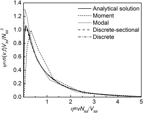
Appendix D

Figure D1 shows the comparison of simulated PSD by the discrete, discrete-sectional, moment and modal models with the analytical solution. Friedlander and Wang (1966) showed that for a purely coagulating system the non-dimensional particle size distribution function becomes independent of initial conditions at long times. This non-dimensional asymptotic distribution is independent of time and is termed self-preserving distribution. We evaluated the accuracy of the coagulation module of the four models by simulating the evolution of PSD with an initially monodisperse aerosol with a size of 1 nm and initial number concentration of 10¹⁶ m⁻³. The simulation was run for 5 s. As seen in this figure, we find very good agreement between the analytical solution (Vemury and Pratsinis 1995) and all four models.

Figure D1. Self-preserving particle size distribution calculated by moment, modal, discrete and discrete-sectional models, compared with analytical solution (Vemury and Pratsinis 1995).

References

- Ackermann, I. J., H. Hass, M. Memmesheimer, A. Ebel, F. S. Binkowski, and U. Shankar. 1998. Modal aerosol dynamics model for Europe: Development and first applications. Atmos. Environ. 32 (17):2981–2999. doi:10.1016/S1352-2310(98)00006-5.
- Binkowski, F. S., and U. Shankar. 1995. The regional particulate matter model: 1. Model description and preliminary results. J. Geophys. Res. 100 (D12):26191–26209. doi:10.1029/95JD02093.
- Biswas, P., C. Y. Wu, M. R. Zachariah, and B. McMillin. 1997. Characterization of iron oxide-silica nanocomposites in flames: Part II. Comparison of discrete-sectional model predictions to experimental data. J. Mater. Res. 12 (3):714–723. doi:10.1557/JMR.1997.0106.
- Brown, D. P., E. I. Kauppinen, J. K. Jokiniemi, S. G. Rubin, and P. Biswas. 2006. A method of moments based CFD model for polydisperse aerosol flows with strong interphase mass and heat transfer. Comput. Fluids 35 (7):762–780. doi:10.1016/j.compfluid.2006.01.012.
- Chadha, T. S., M. Yang, K. Haddad, V. B. Shah, S. Li, and P. Biswas. 2017. Model based prediction of nanostructured thin film morphology in an aerosol chemical vapor deposition process. Chem. Eng. J. 310:102–113. doi:10.1016/j.cej.2016.10.105.
- Fuchs, N. A., and A. G. Sutugin. 1971. Topics in current aerosol research (Part 2), eds. G. M. Hidy and J. R. Brock. New York: Pergamon.
- Frenklach, M., and S. J. Harris. 1987. Aerosol dynamics modeling using the method of moments. J. Colloid Interface Sci. 118 (1):252–261. doi:10.1016/0021-9797(87)90454-1.
- Friedlander, S. K. 2000. Smoke, dust, and haze: Fundamentals of aerosol dynamics. Topics in chemical engineering. New York: Oxford University Press.
- Friedlander, S. K., and C. S. Wang. 1966. The self-preserving particle size distribution for coagulation by Brownian motion. J. Colloid Interface Sci. 22 (2):126–132. doi:10.1016/0021-9797(66)90073-7.
- Gao, Q., S. Li, M. Yang, P. Biswas, and Q. Yao. 2017. Measurement and numerical simulation of ultrafine particle size distribution in the early stage of high-sodium lignite combustion. Proc. Combust. Inst. 36 (2):2083–2090. doi:10.1016/j.proci.2016.07.085.
- Gelbard, F., and J. H. Seinfeld. 1978. Numerical solution of the dynamic equation for particulate systems. J. Comput. Phys. 28 (3):357–375. doi:10.1016/0021-9991(78)90058-X.
- Gelbard, F., and J. H. Seinfeld. 1979. The general dynamic equation for aerosols. Theory and application to aerosol formation and growth. J. Colloid Interface Sci. 68 (2):363–382. doi:10.1016/0021-9797(79)90289-3.
- Gelbard, F., and J. H. Seinfeld. 1980. Simulation of multicomponent aerosol dynamics. J. Colloid Interface Sci. 78 (2):485–501. doi:10.1016/0021-9797(80)90587-1.
- Gelbard, F., Y. Tambour, and J. H. Seinfeld. 1980. Sectional representations for simulating aerosol dynamics. J. Colloid Interface Sci. 76 (2):541–556. doi:10.1016/0021-9797(80)90394-X.
- Geng, J., H. Park, and E. Sajo. 2013. Simulation of aerosol coagulation and deposition under multiple flow regimes with arbitrary computational precision. Aerosol Sci. Technol. 47 (5):530–42. doi:10.1080/02786826.2013.770126.
- Harrington, D. Y., and S. M. Kreidenweis. 1998. Simulations of sulfate aerosol dynamics part ii: Model intercomparison. Atmos. Environ. 32 (10):1701–1709. doi:10.1016/S1352-2310(97)00453-6.
- He, X., Z. Gan, S. Fisenko, D. Wang, H. M. El-Kaderi, and W.-N. Wang. 2017. Rapid formation of metal–organic frameworks (MOFs) based nanocomposites in microdroplets and their applications for CO2 photoreduction. ACS Appl. Mater. Interfaces 9 (11):9688–9698. doi:10.1021/acsami.6b16817.
- Jeong, J. I., and M. Choi. 2003. A simple bimodal model for the evolution of non-spherical particles undergoing nucleation, coagulation and coalescence. J. Aerosol Sci. 34:965–976. doi:10.1016/S0021-8502(03)00067-3.
- Kommu, S., B. Khomami, and P. Biswas. 2004. Simulation of aerosol dynamics and transport in chemically reacting particulate matter laden flows. Part II: Application to CVD reactors. Chem. Eng. Sci. 59 (2):359–371. doi:10.1016/j.ces.2003.05.010.
- Korhonen, H., K. Lehtinen, and M. Kulmala. 2004. Multicomponent aerosol dynamics model UHMA: Model development and validation. Atmos. Chem. Phys. 4 (3):757–771. doi:10.5194/acp-4-757-2004.
- Kruis, F. E., K. A. Kusters, S. E. Pratsinis, and B. Scarlett. 1993. A simple model for the evolution of the characteristics of aggregate particles undergoing coagulation and sintering. Aerosol Sci. Technol. 19 (4):514–526. doi:10.1080/02786829308959656.
- Landgrebe, J. D., and S. E. Pratsinis. 1989. Gas-phase manufacture of particulates: Interplay of chemical reaction and aerosol coagulation in the free-molecular regime. Ind. Eng. Chem. Res. 28 (10):1474–1481. doi:10.1021/ie00094a007.
- Landgrebe, J. D., and S. E. Pratsinis. 1990. A discrete-sectional model for particulate production by gas-phase chemical reaction and aerosol coagulation in the free-molecular regime. J. Colloid Interface Sci. 139 (1):63–86. doi:10.1016/0021-9797(90)90445-T.
- Lee, K., J. Chen, and J. Gieseke. 1984. Log-normally preserving size distribution for Brownian coagulation in the free-molecule regime. Aerosol Sci. Technol. 3 (1):53–62. doi:10.1080/02786828408958993.
- Lehtinen, K., and M. Kulmala. 2003. A model for particle formation and growth in the atmosphere with molecular resolution in size. Atmos. Chem. Phys. 3 (1):251–257. doi:10.5194/acp-3-251-2003.
- Lin, L.-Y., S. Kavadiya, B. B. Karakocak, Y. Nie, R. Raliya, S. T. Wang, M. Y. Berezin, and P. Biswas. 2018. Zno1− x/carbon dots composite hollow spheres: Facile aerosol synthesis and superior CO2 photoreduction under UV, visible and near-infrared irradiation. Appl. Catal. B: Environ. 230:36–48. doi:10.1016/j.apcatb.2018.02.018.
- Lin, L.-Y., Y. Nie, S. Kavadiya, T. Soundappan, and P. Biswas. 2017. N-doped reduced graphene oxide promoted nano TiO2 as a bifunctional adsorbent/photocatalyst for CO2 photoreduction: Effect of N species. Chem. Eng. J. 316:449–460. doi:10.1016/j.cej.2017.01.125.
- Lin, W. Y., V. Sethi, and P. Biswas. 1992. Multicomponent aerosol dynamics of the Pb-O2 system in a bench scale flame incinerator. Aerosol Sci. Technol. 17 (2):119–133. doi:10.1080/02786829208959565.
- Marchisio, D. L., and R. O. Fox. 2005. Solution of population balance equations using the direct quadrature method of moments. J. Aerosol Sci. 36 (1):43–73. doi:10.1016/j.jaerosci.2004.07.009.
- McGraw, R. 1997. Description of aerosol dynamics by the quadrature method of moments. Aerosol Sci. Technol. 27 (2):255–265. doi:10.1080/02786829708965471.
- Moniruzzaman, C. G., and K. Y. Park. 2006. A discrete-sectional model for particle growth in aerosol reactor: Application to titania particles. Korean J. Chem. Eng. 23 (1):159–166. doi:10.1007/BF02705709.
- Mukherjee, D., A. Prakash, and M. Zachariah. 2006. Implementation of a discrete nodal model to probe the effect of size-dependent surface tension on nanoparticle formation and growth. J. Aerosol Sci. 37 (10):1388–1399. doi:10.1016/j.jaerosci.2006.01.008.
- Otto, E., H. Fissan, S. Park, and K. Lee. 1999. The log-normal size distribution theory of brownian aerosol coagulation for the entire particle size range: Part II—Analytical solution using Dahneke’s coagulation kernel. J. Aerosol Sci. 30 (1):17–34. doi:10.1016/S0021-8502(98)00038-X.
- Otto, E., F. Stratmann, H. Fissan, S. Vemury, and S. E. Pratsinis. 1994. Quasi-self-preserving log-normal size distributions in the transition regime. Part. Part. Syst. Charact. 11 (5):359–366. doi:10.1002/ppsc.19940110502.
- Panda, S., and S. E. Pratsinis. 1995. Modeling the synthesis of aluminum particles by evaporation-condensation in an aerosol flow reactor. Nanostruct. Mater. 5:755–767. doi:10.1016/0965-9773(95)00292-M.
- Pirjola, L., M. Kulmala, M. Wilck, A. Bischoff, F. Stratmann, and E. Otto. 1999. Formation of sulphuric acid aerosols and cloud condensation nuclei: An expression for significant nucleation and model comparison. J. Aerosol Sci. 30 (8):1079–1094. doi:10.1016/S0021-8502(98)00776-9.
- Prakash, A., A. Bapat, and M. Zachariah. 2003. A simple numerical algorithm and software for solution of nucleation, surface growth, and coagulation problems. Aerosol Sci. Technol. 37 (11):892–898. doi:10.1080/02786820300933.
- Pratsinis, S. E. 1988. Simultaneous nucleation, condensation, and coagulation in aerosol reactors. J. Colloid Interface Sci. 124 (2):416–427. doi:10.1016/0021-9797(88)90180-4.
- Randolph, A. D., and M. A. Larson. 1971. Theory of particulate processes. New York, NY: Academic Press.
- Riemer, N., M. West, R. A. Zaveri, and R. C. Easter. 2009. Simulating the evolution of soot mixing state with a particle-resolved aerosol model. J. Geophys. Res. 114 (D9):D09202. doi:10.1029/2008JD011073.
- Sandu, A. 2006. Piecewise polynomial solutions of aerosol dynamic equation. Aerosol Sci. Technol. 40 (4):261–273. doi:10.1080/02786820500543274.
- Schild, A., A. Gutsch, H. Mühlenweg, and S. Pratsinis. 1999. Simulation of nanoparticle production in premixed aerosol flow reactors by interfacing fluid mechanics and particle dynamics. J. Nanopart. Res. 1 (2):305–315.
- Seigneur, C., A. B. Hudischewskyj, J. H. Seinfeld, K. T. Whitby, E. R. Whitby, J. R. Brock, and H. M. Barnes. 1986. Simulation of aerosol dynamics: A comparative review of mathematical models. Aerosol Sci. Technol. 5 (2):205–222. doi:10.1080/02786828608959088.
- Seinfeld, J. H., and S. N. Pandis. 2016. Atmospheric chemistry and physics: From air pollution to climate change. New Jersey: John Wiley and Sons.
- Sharma, G., S. Dhawan, N. Reed, R. Chakrabarty, and P. Biswas. 2019. Collisional growth rate and correction factor for TiO2 nanoparticles at high temperatures in free molecular regime. J. Aerosol Sci. 127:27–37. doi:10.1016/j.jaerosci.2018.10.002.
- Sharma, G., Y. Wang, R. Chakrabarty, and P. Biswas. 2019. Modeling simultaneous coagulation and charging of nanoparticles at high temperatures using the method of moments. J. Aerosol Sci. 132:70–82. doi:10.1016/j.jaerosci.2019.03.011.
- Smith, A. J., C. G. Wells, and M. Kraft. 2018. A new iterative scheme for solving the discrete Smoluchowski equation. J. Comput. Phys. 352:373–387. doi:10.1016/j.jcp.2017.09.045.
- Suh, S.-M., M. Zachariah, and S. Girshick. 2001. Modeling particle formation during low-pressure silane oxidation: Detailed chemical kinetics and aerosol dynamics. J. Vac. Sci. Technol. A 19 (3):940–951. doi:10.1116/1.1355757.
- Suriyawong, A., X. Chen, and P. Biswas. 2010. Nano-structured sorbent injection strategies for heavy metal capture in combustion exhausts. Aerosol Sci. Technol. 44 (8):676–691. doi:10.1080/02786826.2010.485589.
- Talukdar, S. S., and M. T. Swihart. 2004. Aerosol dynamics modeling of silicon nanoparticle formation during silane pyrolysis: A comparison of three solution methods. J. Aerosol Sci. 35 (7):889–908. doi:10.1016/j.jaerosci.2004.02.004.
- Tsantilis, S., H. Kammler, and S. Pratsinis. 2002. Population balance modeling of flame synthesis of titania nanoparticles. Chem. Eng. Sci. 57 (12):2139–2156. doi:10.1016/S0009-2509(02)00107-0.
- Vemury, S., and S. E. Pratsinis. 1995. Self-preserving size distributions of agglomerates. J. Aerosol Sci. 26 (2):175–85. doi:10.1016/0021-8502(94)00103-6.
- Wang, Y., G. Sharma, C. Koh, V. Kumar, R. Chakrabarty, and P. Biswas. 2017. Influence of flame-generated ions on the simultaneous charging and coagulation of nanoparticles during combustion. Aerosol Sci. Technol. 51 (7):833–844. doi:10.1080/02786826.2017.1304635.
- Wang, Y., J. Fang, M. Attoui, T. S. Chadha, W. -N. Wang, and P. Biswas. 2014. Application of half mini DMA for Sub 2 nm particle size distribution measurement in an electrospray and a flame aerosol reactor. J. Aerosol Sci. 71:52–64. doi:10.1016/j.jaerosci.2014.01.007.
- Williams, M. 1986. Some topics in nuclear aerosol dynamics. Prog. Nucl. Energy 17 (1):1–52. doi:10.1016/0149-1970(86)90041-7.
- Wright, D., S. Yu, P. Kasibhatla, R. McGraw, S. Schwartz, V. Saxena, and G. Yue. 2002. Retrieval of aerosol properties from moments of the particle size distribution for kernels involving the step function: Cloud droplet activation. J. Aerosol Sci. 33 (2):319–337. doi:10.1016/S0021-8502(01)00172-0.
- Wu, C.-Y., and P. Biswas. 1998. Study of numerical diffusion in a discrete-sectional model and its application to aerosol dynamics simulation. Aerosol Sci. Technol. 29 (5):359–378. doi:10.1080/02786829808965576.
- Wu, J. J., and R. C. Flagan. 1988. A discrete-sectional solution to the aerosol dynamic equation. J. Colloid Interface Sci. 123:339–352. doi:10.1016/0021-9797(88)90255-X.
- Xiong, Y., M. K. Akhtar, and S. E. Pratsinis. 1993. Formation of agglomerate particles by coagulation and sintering—Part II. The evolution of the morphology of aerosol-made titania, silica and silica-doped titania powders. J. Aerosol Sci. 24 (3):301–313. doi:10.1016/0021-8502(93)90004-S.
- Xiong, Y., and S. E. Pratsinis. 1993. Formation of agglomerate particles by coagulation and sintering—Part I. A two-dimensional solution of the population balance equation. J. Aerosol Sci. 24 (3):283–300. doi:10.1016/0021-8502(93)90003-R.
- Yamamoto, M. 2014. A moment method of the log-normal size distribution with the critical size limit in the free-molecular regime. Aerosol Sci. Technol. 48 (7):725–737. doi:10.1080/02786826.2014.922161.
- Yu, F., G. Luo, and X. Ma. 2012. Regional and global modeling of aerosol optical properties with a size, composition, and mixing state resolved particle microphysics model. Atmos. Chem. Phys. 12 (13):5719–5736. doi:10.5194/acp-12-5719-2012.
- Yu, S., P. S. Kasibhatla, D. L. Wright, S. E. Schwartz, R. McGraw, and A. Deng. 2003. Moment‐based simulation of microphysical properties of sulfate aerosols in the eastern United States: Model description, evaluation, and regional analysis. J. Geophys. Res. 108 (D12):4353. doi:10.1029/2002JD002890.
- Yu, S., R. Mathur, J. Pleim, D. Wong, R. Gilliam, K. Alapaty, C. Zhao, and X. Liu. 2014. Aerosol indirect effect on the grid-scale clouds in the two-way coupled WRF-CMAQ: Model description, development, evaluation and regional analysis. Atmos. Chem. Phys. 14 (20):11247–11285. doi:10.5194/acpd-13-25649-2013.
- Zhang, Q., G. Sharma, J. P. Wong, A. Y. Davis, M. S. Black, P. Biswas, and R. J. Weber. 2018. Investigating particle emissions and aerosol dynamics from a consumer fused deposition modeling 3d printer with a lognormal moment aerosol model. Aerosol Sci. Technol. 52 (10):1099–1111. doi:10.1080/02786826.2018.1464115.
- Zhang, Y., C. Seigneur, J. H. Seinfeld, M. Z. Jacobson, and F. S. Binkowski. 1999. Simulation of aerosol dynamics: A comparative review of algorithms used in air quality models. Aerosol Sci. Technol. 31 (6):487–514. doi:10.1080/027868299304039.
- Zhu, S., K. N. Sartelet, and C. Seigneur. 2015. A size-composition resolved aerosol model for simulating the dynamics of externally mixed particles: SCRAM (v 1.0). Geosci. Model Dev. 8 (6):1595–1612. doi:10.5194/gmd-8-1595-2015.