Stochastic effects in H₂SO₄-H₂O cluster growth

Abstract

The nucleation of sulfuric acid-water clusters plays a significant role in the formation of aerosols. Based on a recently developed particle Monte Carlo (MC) Code, we analyze how the growth of sulfuric acid-water clusters is influenced by stochastic fluctuations. We here consider samples of H₂SO₄-H₂O clusters at T = 200 K with a relative humidity of 50%, with particle concentrations between 10⁵ and 10⁷ cm^–3 in volumes between 10^–6 and 10^–2 cm³. We present the temporal evolution of the formation rate and of the size distribution as well as growth rates and the onset time of the nucleation above a given cluster size with and without constant production of new monomers. Clear evidence is revealed by the MC code that fluctuations result in a faster growth rate of the smallest clusters compared to deterministic continuum models that do not contain the stochastic effects. The faster growth of small clusters in turn influences the growth of larger clusters. Depending on the volume size, the onset time for clusters larger than 0.85 nm varies between 1000 s and 20,000 s for $n={10}^5$ cm^–3 and between 10 s and 100 s for $n={10}^7$ cm^–3.

Copyright © 2020 American Association for Aerosol Research

EDITOR:

• Jim Smith

1. Introduction

On a global scale approximately half of cloud condensation nuclei (CCN)—the seeds for cloud droplet formation—originate from nucleation and condensation of low-volatility gases in the modern day atmosphere (Merikanto et al. 2009; Yu and Luo 2009); this number increases to about two thirds for the pre-industrial atmosphere (Gordon et al. 2017). Since newly formed aerosols are small in size (∼1 nm) and thus have a high mobility, they have a high risk of being scavenged by larger particles (Pierce and Adams 2007) before they can grow to sizes relevant for cloud formation. The faster the aerosols can grow to larger sizes the higher their probability of survival so the dynamics of both the formation and growth of new aerosols are therefore important to understand the global CCN concentration (Pierce and Adams 2009).

Traditionally the dynamics of aerosol populations are described by the general dynamic equation (GDE). The continuous equation only treating condensation and evaporation (thus neglecting coagulation, losses to other processes, and production of new monomers) is: (1) $$\frac{\partial c(i,t)}{\partial t}=-\frac{\partial }{\partial i}[(\beta (i)C-\gamma (i))c(i,t)]$$(1) where c is the concentration as a function of size (i), β and γ the condensation and evaporation constants respectively, and C the monomer concentration. Recently it was shown that the inclusion of stochastic fluctuations to the size distribution can significantly increase the calculated growth rates of sub 5-nanometer sized aerosols (Olenius et al. 2018). Stochastic fluctuations can be understood as the random collisions between molecular clusters (and corresponding evaporations) which happen outside of the average growth of the system given by the term $\beta C-\gamma .$ These events are not included in the continuous GDE (Equation (1)(1) $$\frac{\partial c(i,t)}{\partial t}=-\frac{\partial }{\partial i}[(\beta (i)C-\gamma (i))c(i,t)]$$(1) ), which forms the foundation for many aerosol growth models (Olenius et al. 2013; Tröstl et al. 2016).

Not including the stochastic term can thus have the risk of underestimating the potential of nucleated aerosols to form CCN, but this is still a relatively unexplored area. This work is the first application of a recently developed 3D particle Monte Carlo model, tracking individual clusters. Such a model is capable of capturing the individual behavior of each cluster and is therefore suitable to investigate the effects of stochastic fluctuations on a developing aerosol population whilst traditional models such as the classical thermodynamic nucleation theory (Hamill et al. 1982), kinetic models (Pirjola and Kulmala 1998; Lovejoy, Curtius, and Froyd 2004; Yu 2006), nucleation theory (Vehkamäki et al. 2002), or Atmospheric Cluster Dynamics (McGrath et al. 2012) only capture macroscopic or averaged quantities and are therefore not suited to deal with the stochastics of particle growth. The model used was previously described in Köhn, Enghoff, and Svensmark (2018) with modifications as noted in Section 2 where we also describe the setup and simulation runs. In Section 3, we present results on the temporal evolution of the size distribution and its dependence on simulation parameters such as monomer density and simulation volume. Modeled growth rates are compared with those expected from the continuous GDE and we analyze the condensation rates in an attempt to determine the critical cluster size. Finally, we summarize and conclude our study in Section 4. In addition, we describe details about the parallelization of our computational model, which is encoded in Python, in Appendix A.

2. Modeling

We model the motion and clustering of hydrated sulfuric acid clusters as described in detail in Köhn, Enghoff, and Svensmark (2018) where a cluster (H₂SO₄)_i-(H₂O)_j consists of H₂SO₄ molecules and implicitly includes a size dependent amount of H₂O molecules. Here we recapitulate the main features of our simulations: We trace individual particles of given size and update their position through (2) $$\mathbf{r}(t+\Delta t)=\mathbf{r}(t)+\sqrt{2D(R)\Delta t}\mathbf{G}$$(2) with the size-dependent diffusion coefficient D(R) and the time step $\Delta t$ (3) $$D(R)=D_0·{\left(\frac{R(1)}{R}\right)}^2$$(3) (4) $$D_0=\frac{2}{3}\sqrt{\frac{k_B^3{T}^3}{{\pi }^{3}m(1)}}\frac{1}{4PR{(1)}^2}$$(4) (5) $$\Delta t\lesssim \frac{1}{2D_0\sqrt[3]{n^2}}$$(5) for molecules of size R where $R(1)=0.329$ nm and $m(1)=2.0033·{10}^{-25}$ kg are the initial size and the mass of single sulfuric acid molecules without any attached water molecules. $k_B\approx 1.38·{10}^{-23}$ J/K is the Boltzmann constant and P = 1 bar the ambient pressure. For T = 200 K the diffusion coefficient is $D_0\approx 8.96·{10}^{-7}$ m²/s. G is the Gaussian random number $\mathbf{G}=(\varrho \hspace{0.17em}\text{cos}\hspace{0.17em}\varphi \hspace{0.17em}\text{sin}\hspace{0.17em}\theta ,\varrho \hspace{0.17em}\text{sin}\hspace{0.17em}\varphi \hspace{0.17em}\text{sin}\hspace{0.17em}\theta ,\varrho \hspace{0.17em}\text{cos}\hspace{0.17em}\theta )$ with $\varrho =\sqrt{-2\hspace{0.17em}\text{log}\hspace{0.17em}(r_1)},\varphi =2\pi r_2,\theta =\arccos (2r_3-1),r_i\in [0,1).$ The typical time steps for densities between 10⁵ and 10⁷ cm^–3 lie in the order of ${10}^{-2}-{10}^{-3}$ s. With these time steps, the diffusive length scale varies from 42 and 134 μm. Since the mean free path of sulfuric acid molecules in air is approximately 10–60 nm (Seinfeld and Pandis 2006), hence significantly smaller than 1 μm, the justification of the diffusion approach in this study is justified.

After every time step, we check whether clusters evaporate or whether two clusters collide, and if so, determine the mass and volume of the merged cluster.

Throughout this article, we connect the particle size to the number i of H₂SO₄ molecules in the cluster (Yu 2005). In this sense, the particle radius of clusters with i monomers is (6) $$R(i,T)=\sqrt[3]{\frac{3m(i)}{4\pi \varrho (i,T)}}$$(6) Implicitly including the size dependent amount of H₂O molecules found at a relative humidity of approx. 50%. The mass and the density for temperatures between 233 and 323 K are given as in Vehkamäki et al. (2002): (7) $$m(i)=\frac{0.098\frac{\text{kg}}{\text{mol}}}{N_A}·i+\frac{0.018\frac{\text{kg}}{\text{mol}}}{N_A}\mathrm{ }\text{kg}·\frac{i-i·\mathcal{M}\mathcal{F}(i)}{\mathcal{M}\mathcal{F}(i)}$$(7) (8) $$\begin{array}{c}\varrho (i,T)\left[\frac{\text{kg}}{{\text{cm}}^3}\right]=[0.7681724+2.184714·\mathcal{M}\mathcal{F}(i)+7.163002·\mathcal{M}\mathcal{F}{(i)}^2-44.31447·\mathcal{M}\mathcal{F}{(i)}^3+88.75606·\mathcal{M}\mathcal{F}{(i)}^4\\ -75.73729·\mathcal{M}\mathcal{F}{(i)}^5+23.43228·\mathcal{M}\mathcal{F}{(i)}^6+T\left[\mathrm{K}\right]·(0.001808255-0.009294656·\mathcal{M}\mathcal{F}(i)\\ -0.03742147·\mathcal{M}\mathcal{F}{(i)}^2+0.2565321·\mathcal{M}\mathcal{F}{(i)}^3-0.5362872·\mathcal{M}\mathcal{F}{(i)}^4+0.4857736·\mathcal{M}\mathcal{F}{(i)}^5\\ -0.1629592·\mathcal{M}\mathcal{F}{(i)}^6)+T{\left[\mathrm{K}\right]}^2·(-0.000003478524+0.00001335867·\mathcal{M}\mathcal{F}(i)\\ +0.00005195706·\mathcal{M}\mathcal{F}{(i)}^2-0.0003717636·\mathcal{M}\mathcal{F}{(i)}^3+0.0007990811·\mathcal{M}\mathcal{F}{(i)}^4\\ -0.000745806·\mathcal{M}\mathcal{F}{(i)}^5+0.000258139·\mathcal{M}\mathcal{F}{(i)}^6)]\frac{1}{1000}\end{array}$$(8) with the Avogadro constant $N_A\approx 6.022·{10}^{23}$ mol^–1 and the mole fraction (9) $$\mathcal{M}\mathcal{F}(i)=0.4505·i^{-0.2097}$$(9) which is a powerlaw fit to Fig. 2b of Yu (2005) for a temperature of approx. 300 K for a humidity of 50%. Since we here investigate the nucleation of clusters at 200 K only, we multiply Equation (9)(9) $$\mathcal{M}\mathcal{F}(i)=0.4505·i^{-0.2097}$$(9) with a factor of $\approx 0.8$ according to the same figure in Yu (2005). 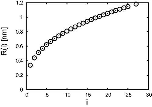As an overview, Figure 1 illustrates Equation (6)(6) $$R(i,T)=\sqrt[3]{\frac{3m(i)}{4\pi \varrho (i,T)}}$$(6) showing the relation between the number i of H₂SO₄ molecules and the radius R of such clusters.

Figure 1. The radius (Equation (6)(6) $$R(i,T)=\sqrt[3]{\frac{3m(i)}{4\pi \varrho (i,T)}}$$(6) ) of H₂SO₄-H₂O clusters as a function of the number i of H₂SO₄ molecules.

Particles collide if the difference between their positions is smaller than the sum of their radii. Once two particles collide, we merge them and update their mass as well as size according to Equations (6)(6) $$R(i,T)=\sqrt[3]{\frac{3m(i)}{4\pi \varrho (i,T)}}$$(6) and (7)(7) $$m(i)=\frac{0.098\frac{\text{kg}}{\text{mol}}}{N_A}·i+\frac{0.018\frac{\text{kg}}{\text{mol}}}{N_A}\mathrm{ }\text{kg}·\frac{i-i·\mathcal{M}\mathcal{F}(i)}{\mathcal{M}\mathcal{F}(i)}$$(7) . During their lifetime, clusters can also evaporate and emit a monomer. After every time step, we check for evaporation through $r\le 1-\hspace{0.17em}\text{exp}\hspace{0.17em}(-\gamma \Delta t)$ where r is a uniform random number $r\in [0,1)$ and where the evaporation rate (Yu 2005) is: (10) $$\gamma (i)=\sqrt{\frac{8\pi k_{B}T(m(1)+m(i))}{m(1)m(i)}}{\left(R(1)+R(i,T)\right)}^2{n}_{a,\mathit{sol}}^{\infty }(i,T)\hspace{0.17em}\text{exp}\hspace{0.17em}\left(\frac{2M_1\sigma (i,T)}{\varrho (i,T)·\mathcal{R}·TR(i,T)}\right)$$(10) where $M_1=98$ g mol^–1 is the molar mass of H₂SO₄, $\mathcal{R}\approx 8.31$ J (mol K)^–1 the universal gas constant, and the concentration $n_{a,\mathit{sol}}^{\infty }$ of H₂SO₄ vapor molecules in the equilibrium vapor above a flat source and the surface tension σ for temperatures between 273 and 373 K are determined through (Noppel, Vehkamäki, and Kulmala 2002; Vehkamäki et al. 2002): (11) $$n_{a,\mathit{sol}}^{\infty }(i,T)\left[{\mathrm{m}}^{-3}\right]=0.0017241·\mathcal{M}\mathcal{F}{(i)}^{10.891}·\frac{133}{T\left[\mathrm{k}\right]·\mathcal{R}}·N_A$$(11) (12) $$\begin{array}{c}\sigma (i)\left[\mathrm{N}{\mathrm{m}}^{-1}\right]=0.11864-0.11651·\mathcal{M}\mathcal{F}(i)+0.76852·\mathcal{M}\mathcal{F}{(i)}^2-2.40909·\mathcal{M}\mathcal{F}{(i)}^3+2.95434·\mathcal{M}\mathcal{F}{(i)}^4\\ -1.25852·\mathcal{M}\mathcal{F}{(i)}^5+T\left[\mathrm{k}\right]·(-0.00015709+0.00040105·\mathcal{M}\mathcal{F}(i)-0.0023995·\mathcal{M}\mathcal{F}{(i)}^2\\ +0.007611235·\mathcal{M}\mathcal{F}{(i)}^3-0.00937386·\mathcal{M}\mathcal{F}{(i)}^4+0.00389722·\mathcal{M}\mathcal{F}{(i)}^5)\end{array}$$(12)

Because of the lack of physical data, e.g., for the equilibrium vapor pressure, we still use Equations (8(8) $$\begin{array}{c}\varrho (i,T)\left[\frac{\text{kg}}{{\text{cm}}^3}\right]=[0.7681724+2.184714·\mathcal{M}\mathcal{F}(i)+7.163002·\mathcal{M}\mathcal{F}{(i)}^2-44.31447·\mathcal{M}\mathcal{F}{(i)}^3+88.75606·\mathcal{M}\mathcal{F}{(i)}^4\\ -75.73729·\mathcal{M}\mathcal{F}{(i)}^5+23.43228·\mathcal{M}\mathcal{F}{(i)}^6+T\left[\mathrm{K}\right]·(0.001808255-0.009294656·\mathcal{M}\mathcal{F}(i)\\ -0.03742147·\mathcal{M}\mathcal{F}{(i)}^2+0.2565321·\mathcal{M}\mathcal{F}{(i)}^3-0.5362872·\mathcal{M}\mathcal{F}{(i)}^4+0.4857736·\mathcal{M}\mathcal{F}{(i)}^5\\ -0.1629592·\mathcal{M}\mathcal{F}{(i)}^6)+T{\left[\mathrm{K}\right]}^2·(-0.000003478524+0.00001335867·\mathcal{M}\mathcal{F}(i)\\ +0.00005195706·\mathcal{M}\mathcal{F}{(i)}^2-0.0003717636·\mathcal{M}\mathcal{F}{(i)}^3+0.0007990811·\mathcal{M}\mathcal{F}{(i)}^4\\ -0.000745806·\mathcal{M}\mathcal{F}{(i)}^5+0.000258139·\mathcal{M}\mathcal{F}{(i)}^6)]\frac{1}{1000}\end{array}$$(8) ) and (12(12) $$\begin{array}{c}\sigma (i)\left[\mathrm{N}{\mathrm{m}}^{-1}\right]=0.11864-0.11651·\mathcal{M}\mathcal{F}(i)+0.76852·\mathcal{M}\mathcal{F}{(i)}^2-2.40909·\mathcal{M}\mathcal{F}{(i)}^3+2.95434·\mathcal{M}\mathcal{F}{(i)}^4\\ -1.25852·\mathcal{M}\mathcal{F}{(i)}^5+T\left[\mathrm{k}\right]·(-0.00015709+0.00040105·\mathcal{M}\mathcal{F}(i)-0.0023995·\mathcal{M}\mathcal{F}{(i)}^2\\ +0.007611235·\mathcal{M}\mathcal{F}{(i)}^3-0.00937386·\mathcal{M}\mathcal{F}{(i)}^4+0.00389722·\mathcal{M}\mathcal{F}{(i)}^5)\end{array}$$(12) ) for T = 200 K and multiply Equation (10)(10) $$\gamma (i)=\sqrt{\frac{8\pi k_{B}T(m(1)+m(i))}{m(1)m(i)}}{\left(R(1)+R(i,T)\right)}^2{n}_{a,\mathit{sol}}^{\infty }(i,T)\hspace{0.17em}\text{exp}\hspace{0.17em}\left(\frac{2M_1\sigma (i,T)}{\varrho (i,T)·\mathcal{R}·TR(i,T)}\right)$$(10) with a factor of $\approx {10}^{-5}$ for 200 K based on Fig. 4 of Yu (2005) where evaporation rates for different temperatures and humidities are depicted. For more details, we refer to Köhn, Enghoff, and Svensmark (2018).

We have performed simulations for initial concentrations of $n={10}^5$ cm^–3 up to $n={10}^7$ cm^–3 particles with one central sulfuric acid molecule in domains of size $V={10}^{-6}$-${10}^{-2}$ cm³ such that for each particle concentration n we run simulations with $N_0=n·V=10-1000$ initial particles. We here use periodic boundary conditions such that particles which leave the simulation domain on one side enter the simulation domain on the opposite side. For each set-up, we run three different simulations with different realizations of random numbers. All the results presented in Section 3 are then averaged over these three runs such that we can exclude that our findings are influenced by numerical noise.

We run simulations with and without monomer production. In the first case, we add one H₂SO₄-H₂O monomer whenever merging two particles reduces the total particle number below N₀. Thus, we ensure that the particle number and the particle concentration stay constant. However, in cases of evaporation, the emitted molecule is added to the simulation domain and the particle density slightly increases. Yet in all considered cases, we have observed that the growth of the concentration of all particles is negligible and does not change our conclusions. In the second case, we do not add particles to the simulation domain if the particle number decreases below N₀; hence, the gas depletes and, if the simulation ran sufficiently long enough, we would end up with one cluster containing all the initial molecules.

All simulations are performed in Python. Since such simulations can take from days up to several weeks, depending on the physical time and on the number of particles, the code has been parallelized as described in detail in Appendix A.

3. Results

3.1. Dependence of the formation rate on the volume

Figure 2 shows the formation rate of clusters with a radius larger than 0.85 nm at 200 K for different initial cluster concentrations and for different domain volumes. The size is chosen since R = 0.85 nm is comparable to the size of nucleated clusters for the sulfuric acid-water system used in several large parameterizations (Dunne et al. 2016; Gordon et al. 2017; Tomicic, Enghoff, and Svensmark 2018), although measurements at even smaller sizes also are possible (Kontkanen et al. 2017). The left column of Figure 2 shows the formation rates when keeping the particle density constant whilst the second column shows the formation rate when the total particle number decreases in time as a result of particle merging. Comparing the panels within each column shows that increasing the initial particle concentrations increases the formation rate. Additionally, the particles start to cluster earlier for increased particle concentrations. In the left column, hence for simulations with constant particle production, the dotted lines show the parameterized formation rate deducted from experiments by Dunne et al. (2016), see Appendix B. As shown in Köhn, Enghoff, and Svensmark (2018), our simulation results develop asymptotically against the parameterized formation rate and agree well within one order of magnitude.

Figure 2. The formation rate of H₂SO₄-H₂O clusters larger than R = 0.85 nm for different initial densities with (first column) and without (second column) constant particle production. The dotted lines show the formation rates (20) from the parameterization summarized in Appendix B.

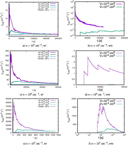
Each panel shows the formation rates for one particle concentration, but for different domain sizes. Note that the formation rate for $n={10}^6$ cm^–3 and $V={10}^{-3}$ cm³ is initially so small such that it is barely visible in panels c and d. The comparison for different volumes demonstrates that the formation rates tend to one asymptotic value for each particle concentration irrespective of the domain size. However, the temporal evolution of $J_{0.85}$ depends significantly on V. Clusters above 0.85 nm appear first in small domain sizes, then later for larger domain sizes. Additionally in small domains, the formation rates increases suddenly, peaks and then decreases toward the asymptotic value whereas the rate in larger volumes grows rather monotonically toward the asymptotic formation rate.

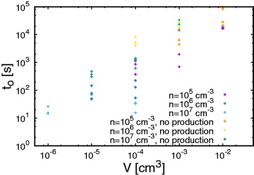
Figure 3 shows the onset time t_O for clusters above 0.85 nm, i.e., the time when the first cluster larger than 0.85 nm appears, for different volumes. Each dot shows the onset time for one particular simulation (three simulations were made for each setting). Note that 12 molecules are needed to form clusters above 0.85 nm; thus in those simulations without particle production where the initial particle number is below 12, clusters above 0.85 nm cannot appear. The general tendency shows that the onset time is smallest for small domain sizes and large for larger domains. However, we also see fluctuations amongst the three different simulations for each combination (n, V) based on the stochastic nature revealed by the Monte Carlo approach. For $V={10}^{-4}$ cm³ and $n={10}^6$ cm^–3 with particle production, the onset time in two simulations is approximately 1300s whilst it is $\approx 600$ s for the third one. For $n={10}^5$ cm^–3 and the same volume, the onset times in three different simulations amount to approx. 1100, 900, and 400 s. Hence, although in two simulations the onset time for $n={10}^6$ cm^–3 is larger than for $n={10}^5$ cm^–3, we have discovered one simulation where clusters above 0.85 nm occur faster than in two simulations for $n={10}^5$ cm^–3. Since we are limited by the runtime of our Monte Carlo code, we cannot run simulations with larger volumes. However, Figure 2 shows that for the largest volumes, the formation rates grow more smoothly than for the smaller volumes. Therefore, we believe that the onset times are sufficiently converged for the largest volumes.

Figure 3. The onset time of clusters larger than 0.85 nm for different concentrations and volumes.

For $n={10}^5$ cm^–3, Table 1 summarizes the onset times for clusters of several different sized (i) in different domain volumes with and without particle production as an average of the three runs for each setting. For small clusters, $i\ge 2$ and $i\ge 3,$ the onset time is comparable for all volumes (irrespective of the particle production). However, for $i\ge 5$ and more significantly for $i\ge 7,$ the onset time increases for larger volumes which proceeds until clusters larger than 0.85 nm or equivalently $i\ge 12.$

Table 1. The onset time [s] of clusters larger than size i for $n={10}^5$ cm^–3 and T = 200 K in different volumes.

	$V={10}^{-4}$ cm^3	$V={10}^{-3}$ cm^3	$V={10}^{-2}$ cm^3	$V={10}^{-3}$ cm^3, no	$V={10}^{-2}$ cm^3, no
$i\ge 2$	1.19 ± 0.78	2.57 ± 1.28	0.99 ± 0.03	1.67 ± 0.95	1.33 ± 0.47
$i\ge 3$	10.39 ± 6.13	7.71 ± 3.23	18.32 ± 15.70	9.01 ± 5.89	11.67 ± 9.46
$i\ge 5$	61.10 ± 16.35	177.88 ± 43.10	518.135 ± 98.115	210.01 ± 65.16	223.01 ± 105.76
$i\ge 7$	132.97 ± 61.90	471.25 ± 108.60	2038.91 ± 318.89	954.01 ± 578.15	1895.01 ± 796.19

The first three columns show results for simulations with monomer production, the last two columns show results without monomer production.

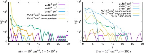
In the following, we discuss what causes these differences by the way of the example for $n={10}^5$ cm^–3: Figure 4 shows the size distributions after different time steps with and without particle production. It demonstrates that cluster growth is more efficient in small domains. After $5·{10}^3$ s, the largest cluster has a size of i = 27 in a domain of $V={10}^{-4}$ cm³ when particles are added to the simulation domain. Note that for a particle concentration of $n={10}^5$ cm^–3 and a volume of $V={10}^{-4}$ cm³, there are only ten particles in the simulation domain. However, we add one monomer after every collision; hence clusters can become larger than i = 10. After $5·{10}^3$ s, the second largest clusters are found in a domain of size $V={10}^{-3}$ cm³, followed by the domain of size $V={10}^{-2}$ cm³. In large domain, the size distributions are much smoother than in small domains because of the larger number of particles. The same tendency holds if no particles are added to the simulation domain. Larger clusters are found in smaller domains whereas the size distribution is smoother in larger domains. In comparison to the simulations where particles are added, the clusters are smaller because of the limited number of particles. In this case, the size of the largest cluster can never be larger than the initial number of particles.

Figure 4. The size distribution of all clusters for $n={10}^5$ cm^–3 and different volumes after different time steps. Panel c has a simulation without coagulation (labeled ‘mono’).

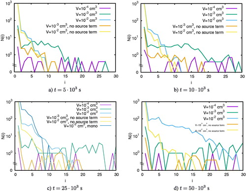
The same tendency holds when the simulation progresses in time (panels b–d). In all considered cases, the largest clusters are found in small simulation volumes. The size distributions in larger domains keep their smooth shape as the cluster size grows. In panel c, a single simulation (the other results are averaged over three simulations) has been added where coagulation was disabled, meaning that only collisions involving at least one monomer were allowed. It is seen that for the initial steps coagulation is not important for this number concentration, whereas the simulation with similar volume including coagulation reaches larger cluster sizes.

Figure 5 shows the size distributions for $n={10}^6$ cm^–3 after 5000s (a) and for $n={10}^7$ cm^–3 after 200 s (b). We observe the same tendencies which we have observed for $n={10}^5$ cm^–3: Small domain sizes favor larger clusters whereas large volumes imply rather smooth size distributions. In panel b, a single simulation without coagulation (similarly to the case in Figure 4c) has been added. Here the effect of lack of coagulation is seen more clearly on the size distribution.

Figure 5. The size distribution of all clusters for (a) $n={10}^6$ cm^–3 and (b) $n={10}^7$ cm^–3 and different volumes. Panel b has a simulation without coagulation (labeled ‘mono’).

To understand this pattern, Figure 6 shows the number of clusters of sizes i = 2, 5, 7, and 12 normalized to the initial particle number N₀ as a function of time for $n={10}^5$ cm^–3 for different volumes with and without particle production. Panel a shows that the normalized number of dimers fluctuates more significantly in small domains irrespective of whether we keep the total particle number constant or whether we take gas depletion into account. For larger cluster sizes, the fluctuations decrease for $V={10}^{-3}-{10}^{-2}$ cm³. Only for $V={10}^{-4}$ are fluctuations still very large compared to larger volumes.

Figure 6. The number of clusters of size i normalized to the initial particle number N₀ as a function of time for $n={10}^5$ cm^–3.

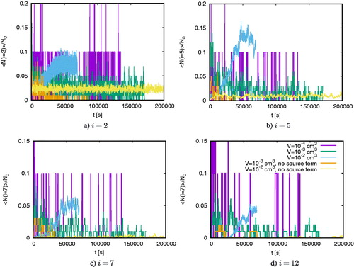
Table 2 shows the mean particle number (13) $$〈N(i)〉=\frac{1}{T}\sum _{t}N(i,t)$$(13) averaged over time of the whole simulation run with the standard deviation (14) $$\Delta N(i)=\sqrt{\frac{1}{T}\sum _t{\left(N(i,t)-〈N(i)〉\right)}^2}.$$(14)

Table 2. The mean particle number $〈N(i)〉$ (13) for different sizes i.

	V=${10}^{-4}$ cm^3	V=${10}^{-3}$ cm^3	V=${10}^{-2}$ cm^3	${10}^{-3}$ cm^3, w/o	${10}^{-2}$ cm^3, w/o
i = 2	1.07 ± 2.25	2.86 ± 1.80	53.48 ± 20.14	2.03 ± 3.64	22.85 ± 4.76
i = 5	1.02 ± 2.55	2.72 ± 2.28	64.78 ± 46.68	1.87 ± 4.21	9.38 ± 2.79
i = 7	1.05 ± 3.42	1.84 ± 1.87	20.86 ± 19.09	1.69 ± 3.51	1.78 ± 1.35
i = 12	1.11 ± 3.08	1.66 ± 1.66	12.98 ± 14.55	1.09 ± 2.04	1.29 ± 1.53

Columns four and five show $〈N(i)〉$ without adding particles.

Table 2 illustrates that for $V={10}^{-4}$ cm³ the standard deviation exceeds the mean particle number. For larger volumes, the standard deviation becomes comparable or smaller than the mean particle number. Such fluctuations in small simulation domains imply that in small simulation domains there is a higher probability to create first dimers and subsequently larger clusters; hence in domains with small volumes, the production of large clusters is accelerated.

3.2. Critical cluster size

The critical cluster size is a central concept in nucleation as it is the size where the cluster becomes stable and is said to nucleate. From the thermodynamic perspective it is the maximum in the Gibbs free energy $\Delta G$ of formation vs r plot occurs (Curtius 2006) or the saddlepoint in a two-component system. From a kinetic standpoint the critical cluster size is where the collision rate equals the evaporation rate. Note that these two sizes are not always exactly the same (Nishioka 1995). This size is extremely dependent on temperature due to the evaporation rate and on the concentration of the condensing gas, due to the collision rate. One way to find the critical cluster size for a given set of parameters is to compare collision and evaporation rates (Yu 2005). In our model the evaporation rates are hard coded, but collision rates are an emergent property so it would be interesting to try to determine the critical cluster size based on model output.

After a simulation has reached equilibrium, i.e., $dN(i)/dt\equiv 0$ for all relevant sizes i, this equilibrium translates to (15) $$0=\gamma \left(i+1\right)·n(i+1)+\theta \left(i-1\right)·n(i-1)-\theta \left(i\right)·n(i)-\gamma \left(i\right)·n(i)$$(15) where γ is the evaporation rate (Equation (10)(10) $$\gamma (i)=\sqrt{\frac{8\pi k_{B}T(m(1)+m(i))}{m(1)m(i)}}{\left(R(1)+R(i,T)\right)}^2{n}_{a,\mathit{sol}}^{\infty }(i,T)\hspace{0.17em}\text{exp}\hspace{0.17em}\left(\frac{2M_1\sigma (i,T)}{\varrho (i,T)·\mathcal{R}·TR(i,T)}\right)$$(10) ), θ the condensation rate ($\beta ·n(1)$) and $n(i)=N(i)/V$ the concentration of clusters of size i. Approximating $\theta (i-1)\approx \theta (i)$ and $\gamma (i)\approx \gamma (i+1)$ allows us to solve for the production rate θ (16) $$\theta (i)=\gamma (i)\frac{N(i)-N(i+1)}{N(i-1)-N(i)}$$(16) which depends on the evaporation rates and on the cluster concentrations and allows us to approximate θ from the output of the simulations. Note that this analysis is related to the standard Becker-Döring derivation (Becker and Döring 1935; Wattis 1999).

Figure 7 shows the evaporation rate (Equation (10)(10) $$\gamma (i)=\sqrt{\frac{8\pi k_{B}T(m(1)+m(i))}{m(1)m(i)}}{\left(R(1)+R(i,T)\right)}^2{n}_{a,\mathit{sol}}^{\infty }(i,T)\hspace{0.17em}\text{exp}\hspace{0.17em}\left(\frac{2M_1\sigma (i,T)}{\varrho (i,T)·\mathcal{R}·TR(i,T)}\right)$$(10) ) and the condensation rate (Equation (16)(16) $$\theta (i)=\gamma (i)\frac{N(i)-N(i+1)}{N(i-1)-N(i)}$$(16) ) with and without coagulation for $n={10}^7$ cm^–3 and $V={10}^{-4}$ cm^–3 for which the formation rate for clusters larger than 0.85 nm is depicted in Figure 2e. It shows that in all considered cases the condensation rate oscillates around the evaporation rate. Note that we still have stochastic fluctuations in the output of our model, therefore $(N(i)-N(i+1)){(N(i-1)-N(i))}^{-1}$ also fluctuates explaining the oscillation of θ; in models, where the N(i) are calculated deterministically, fluctuations would tend to zero. Note also that in some cases $N(i+1)>N(i)$ or equivalently $N(i)>N(i-1)$ such that $\theta <0$ and hence θ is not visible on the logarithmic y-axis. Apart from these constraints, we are able to determine the (first) intersection point between the condensation and evaporation rate indicating the critical cluster size. For the simulation without coagulation, the critical cluster size lies at approx. i = 2 (keeping the stochastic effects in mind) whilst it lies at $i_1=2,i_2=2,$ and $i_3=7$ averaging to $i\approx 4$ which is qualitatively in good agreement with the data presented in Yu (2005). In theory, this method would allow us to determine the critical cluster size for all of the presented simulations if we were not limited by the long runtime of the simulations. Naturally, coagulation plays an important role for the critical cluster size (Ehrhart and Curtius 2013; Malila et al. 2015). Yet, with all the stochastic effects, we are not able to clearly reveal its effect. Note that fluctuations in temperature would lead to additional fluctuations in the critical cluster size (McGraw and LaViolette 1995). However, since the temperature is kept constant in our simulations, this effect is negligible for our considerations.

Figure 7. The evaporation rate (10) and the production rate (16) as a function of cluster size i with and without coagulation for $n={10}^7$ cm^–3 and $V={10}^{-4}$ cm³. Taking coagulation into account, we present results from three simulations with different random numbers.

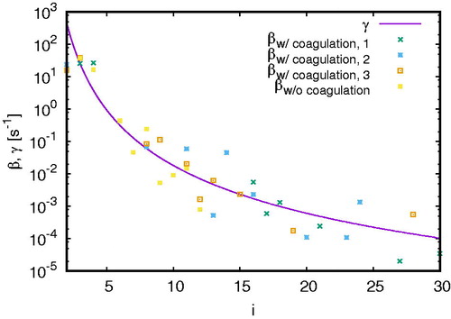
If the stochastic processes contribute significantly to the formation rate of small clusters they could reduce the critical cluster size from a kinetic viewpoint. Since the critical cluster size is defined from ($\Delta G$) this phenomenon is not a true reduction of the critical cluster size, but could perhaps be considered as an effective critical cluster size.

3.3. Growth rates

For $n={10}^5$ cm^–3, Figure 8 compares the growth rate (17) $$G{R}_{\mathit{cond}}(R)=\frac{1}{2\pi \varrho (R(i))R^2}\left(\beta (R(i))n-\gamma (R(i))\right)m(R(i))$$(17)

Figure 8. The comparison of the growth rate GR_cond (17) omitting stochastic effects with the apparent growth rates (18) for different volumes with and without particle production including a single simulation without coagulation for $n={10}^5$ cm^–3.

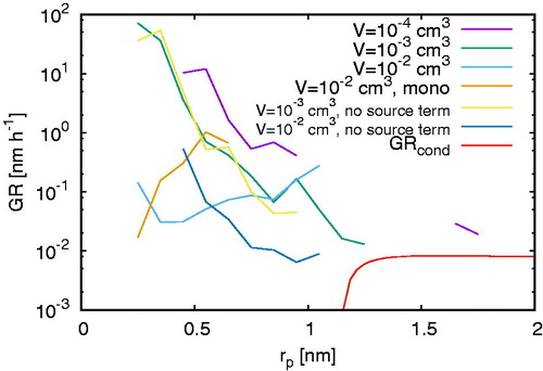
omitting stochastic effects with the apparent growth rate (18) $$G{R}_{\mathit{app}}(R)=\frac{2\Delta R}{\Delta t}$$(18) which is the change of size per time interval and therefore gives us the opportunity to determine the speed of cluster growth in contrast to the formation rate of clusters of a given size or the size distribution for a fixed time step. Whereas Equation (18)(18) $$G{R}_{\mathit{app}}(R)=\frac{2\Delta R}{\Delta t}$$(18) is calculated from our simulation results and therefore distinguishes different volumes and particle production, Equation (17)(17) $$G{R}_{\mathit{cond}}(R)=\frac{1}{2\pi \varrho (R(i))R^2}\left(\beta (R(i))n-\gamma (R(i))\right)m(R(i))$$(17) is calculated analytically and therefore only depends on the particle concentration n, but not on the particle number, i.e., on volumes and source terms. Here ϱ is the density (Equation (8)(8) $$\begin{array}{c}\varrho (i,T)\left[\frac{\text{kg}}{{\text{cm}}^3}\right]=[0.7681724+2.184714·\mathcal{M}\mathcal{F}(i)+7.163002·\mathcal{M}\mathcal{F}{(i)}^2-44.31447·\mathcal{M}\mathcal{F}{(i)}^3+88.75606·\mathcal{M}\mathcal{F}{(i)}^4\\ -75.73729·\mathcal{M}\mathcal{F}{(i)}^5+23.43228·\mathcal{M}\mathcal{F}{(i)}^6+T\left[\mathrm{K}\right]·(0.001808255-0.009294656·\mathcal{M}\mathcal{F}(i)\\ -0.03742147·\mathcal{M}\mathcal{F}{(i)}^2+0.2565321·\mathcal{M}\mathcal{F}{(i)}^3-0.5362872·\mathcal{M}\mathcal{F}{(i)}^4+0.4857736·\mathcal{M}\mathcal{F}{(i)}^5\\ -0.1629592·\mathcal{M}\mathcal{F}{(i)}^6)+T{\left[\mathrm{K}\right]}^2·(-0.000003478524+0.00001335867·\mathcal{M}\mathcal{F}(i)\\ +0.00005195706·\mathcal{M}\mathcal{F}{(i)}^2-0.0003717636·\mathcal{M}\mathcal{F}{(i)}^3+0.0007990811·\mathcal{M}\mathcal{F}{(i)}^4\\ -0.000745806·\mathcal{M}\mathcal{F}{(i)}^5+0.000258139·\mathcal{M}\mathcal{F}{(i)}^6)]\frac{1}{1000}\end{array}$$(8) ), γ the evaporation frequency (Equation (10)(10) $$\gamma (i)=\sqrt{\frac{8\pi k_{B}T(m(1)+m(i))}{m(1)m(i)}}{\left(R(1)+R(i,T)\right)}^2{n}_{a,\mathit{sol}}^{\infty }(i,T)\hspace{0.17em}\text{exp}\hspace{0.17em}\left(\frac{2M_1\sigma (i,T)}{\varrho (i,T)·\mathcal{R}·TR(i,T)}\right)$$(10) ), and for β we use the analytic condensation rate (Yu 2005): (19) $$\beta (R(i))=\sqrt{\frac{8\pi k_{B}T(m(1)+m(R(i)))}{m(1)m(R(i))}}{\left(R(1)+R(i)\right)}^2.$$(19)

Figure 8 shows the presence of two different regimes. For clusters smaller than approximately 1.2 nm, GR_cond tends to zero suggesting that clusters would not grow at all. Above 1.2 nm, GR_cond grows smoothly toward an asymptotic value of approximately ${10}^{-2}$ nm h^–1. The growth rate GR_app (Equation (18)(18) $$G{R}_{\mathit{app}}(R)=\frac{2\Delta R}{\Delta t}$$(18) ) appears to behave similarly to GR_cond for clusters larger than 1.2 nm where it tends to a value close to ${10}^{-2}$ nm h^–1.

However, for clusters smaller than 1.2 nm, GR_cond and GR_app differ significantly. Whilst GR_cond tends to zero, GR_app varies between ${10}^{-2}$ nm h^–1 and 10² nm h^–1 which is due to stochastic effects neglected in GR_cond. Therefore, stochastic effects give a natural explanation why particles initially grow and form larger clusters. If stochastic effects were omitted, the growth rate becomes negative suggesting no cluster growth at all. In almost all considered cases, except for some deviations for $V={10}^{-2}$ cm³, the growth rates are highest for approx. 0.3 nm, the size of clusters with one central sulfuric acid molecule, and decreases as a function of time. Consistent with the fluctuations and size distributions discussed in Section 3.1, the growth rates are largest for small volumes, i.e., a small number of initial particles, and decreases with increasing domain size which is an artifact of the stochastic fluctuations for small volumes. Finally a single simulation (the other results shown are averaged over three simulations) without coagulation (meaning that only collisions involving a monomer are allowed) using the largest volume ($V={10}^{-2}$ cm³) has been performed showing that in this regime it is not coagulation that causes the observed effect.

4. Discussion and conclusion

We have simulated the motion and growth of sulfuric acid-water clusters at 200 K and 1 bar for densities of $n={10}^5$–10⁷ cm^–3 in volumes between ${10}^{-6}$ cm³ and ${10}^{-2}$ cm³. We have observed that growth rates for smaller clusters are significantly larger when stochastic effects are included. Thus, the occurrence onset time of clusters above 0.85 nm varies between approx. 1000 s and 20,000 s for $n={10}^5$ cm^–3 and between 10 and 100 s for $n={10}^7$ cm^–3. Since the formation rates decrease as temperatures increase due to faster evaporation rates, we conclude that the times for nucleation calculated in Section 3.1 can be seen as lower limits only for temperatures relevant to the lower atmosphere.

We have seen that the temporal evolution of the cluster growth depends not only on the initial particle concentration, but also on the volume of the domain size or equivalently on the initial particle number. Smaller domain sizes or equivalently a smaller number of initial particles fluctuate more significantly which in turn favors a faster growth initially of small clusters and subsequently of larger clusters. A comparison of the growth rate of our simulations with the analytic growth rate omitting stochastic effects shows the natural demand for stochastic fluctuations to initiate the growth of the very smallest clusters.

The enhanced initial growth rate can be critical not only for pushing particles past the nucleation barrier, but for growing clusters to larger sizes in general. As scavenging by larger particles is most efficient for the smallest clusters this can improve the survivability of clusters and thus improve their chance of growing to CCN sizes.

In alignment with the dependence of the temporal evolution of the cluster sizes, we have presented a way to calculate the condensation rate θ based on the outcome of the Monte Carlo particle code. By equating θ with the evaporation rate γ, this allows us to estimate the critical cluster size. For a particle concentration of $n={10}^7$ cm^–3 in a volume of ${10}^{-4}$ cm³, we have here determined this critical cluster size to be approximately i = 6 which is in agreement with the critical cluster size determined in Yu (2005). In theory, we could potentially calculate the critical cluster sizes for all considered cases. However, we are here limited by the long runtime of our calculations and by the computational infrastructure such that the concentrations have not reached equilibrium yet. However, in future, computers with faster CPUs, a translation of the applied Monte Carlo code to GPUs or using super computers with a multitude of CPUs would allow us to run simulations faster and therefore reach equilibrium faster.

In conclusion, we have observed that growth rates and formation rates are significantly larger in small volumes where stochastic effects are dominant but that these effects exist across all investigated domain sizes. Stochastic effects are not visible at all in models which are based on averaged quantities only and the inclusion of stochastics would more accurately portray atmospheric processes enhancing the very early stages of aerosol formation and could thus affect the formation of even larger particles.

This study was the first application of a recent 3D Monte Carlo code (Köhn, Enghoff, and Svensmark 2018). In future work, we will extend this code with further species, including ions, and optimize the runtime to further study the spatio-temporal dependence and the influence of dipole–dipole interactions on nucleation processes.

Auhor contributions

All simulations were performed by C.K. Evaluations, interpretations and writing were performed together.

Disclosure statement

There are no competing interests.

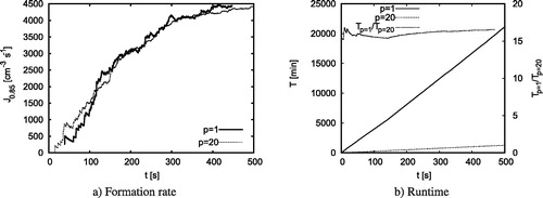
Figure A1. (a) The formation rate $J_{0.85}$ of clusters larger than 0.85 nm as a function of physical time for a particle concentration of $n={10}^7$ cm^–3 in a volume of $V={10}^{-4}$ cm³. The dashed line shows the formation rate from a simulation with one single processor, the dotted line from a parallelized simulation with 20 processors. (b) The runtime T as a function of physical time for simulations with 1 and 20 processors. The right y-axis shows the ratio of the runtime for the two different simulations.

Additional information

Funding

This project has received funding from the European Unions Horizon 2020 research and innovation program under the Marie Sklodowska-Curie grant agreement 722337.

Appendix A: Parallelization in Python

All simulations were performed in Python 2.6.6. In order to optimize runtime, we have parallelized the code with the package “Multiprocessing” with the subpackage “pool”. We initiate a pool of p processors where we distribute all N particles such that each processor advances approximately the same number $N·p^{-1}$ of particles. We have tested the parallelization with a simulation of 1000 particles in a volume of ${10}^{-4}$ cm³, thus $n={10}^7$ cm^–3 running on one processor and on twenty processors.

For this particular set-up, Figure A1a shows the formation rate of clusters above 0.85 nm of the simulation as a function of physical time. It demonstrates that we get comparable results with respect to the formation rate implying that implementing this parallelization into Python does not falsify our results. Panel b shows that the runtime is approximately 16 times faster. The decrease in runtime does not amount to 20 because we have only parallelized the part of the code with respect to particle motion, collision and evaporation. In contrast, overhead procedures such as the input-output of data run only on one processor slowing down the parallelized code slightly.

Appendix B: Parameterizations of formation rates

As parameterization, we use the formation rate $J_{0.85}$ of H₂SO₄-H₂O clusters derived from experiments by Dunne et al. (2016) for temperatures between 208 and 292 K: (B1) $$J\left[{\text{cm}}^{-3}{\mathrm{s}}^{-1}\right]=\hspace{0.17em}\text{exp}\hspace{0.17em}\left(u-v·T\left[\mathrm{K}\right]/1000\right)·n{\left[{10}^6{\text{cm}}^{-3}\right]}^p$$(B1) with (B2) $$u=46.3$$(B2) (B3) $$v=245.0$$(B3) (B4) $$p=3.62$$(B4) for given temperature T and density n (here in units of 10⁶ cm^–3) of initial H₂SO₄-H₂O clusters with one central sulfuric acid molecule.

References

- Becker, R., and W. Döring. 1935. Kinetische Behandlung der Keimbildung in übersättigten Dämpfen. Ann. Phys. 416 (8):719–52. doi:10.1002/andp.19354160806.
- Curtius, J. 2006. Nucleation of atmospheric aerosol particles. C. R. Phys. 7 (9–10):1027–45. doi:10.1016/j.crhy.2006.10.018.
- Dunne, E. M., H. Gordon, A. Kürten, J. Almeida, J. Duplissy, C. Williamson, I. K. Ortega, K. J. Pringle, A. Adamov, U. Baltensperger, et al. 2016. Global atmospheric particle formation from CERN CLOUD measurements. Science 354 (6316):1119–24. doi:10.1126/science.aaf2649,.
- Ehrhart, S., and J. Curtius. 2013. Influence of aerosol lifetime on the interpretation of nucleation experiments with respect to the first nucleation theorem. Atmos. Chem. Phys. 13 (22):11465–71. doi:10.5194/acp-13-11465-2013.
- Gordon, H., J. Kirkby, U. Baltensperger, F. Bianchi, M. Breitenlechner, J. Curtius, A. Dias, J. Dommen, N. M. Donahue, E. M. Dunne, et al. 2017. Causes and importance of new particle formation in the present-day and preindustrial atmospheres. J. Geophys. Res. Atmos. 122 (16):8739–60. doi:10.1002/2017JD026844.
- Hamill, P., R. Turco, C. Kiang, O. Toon, and R. Whitten. 1982. An analysis of various nucleation mechanisms for sulfate particles in the stratosphere. J. Aerosol Sci. 13 (6):561–85. doi:10.1016/0021-8502(82)90021-0.
- Köhn, C., M. Enghoff, and H. Svensmark. 2018. A 3D particle Monte Carlo approach to studying nucleation. J. Comput. Phys. 363:30–8. doi:10.1016/j.jcp.2018.02.032.
- Kontkanen, J., K. Lehtipalo, L. Ahonen, J. Kangasluoma, H. E. Manninen, J. Hakala, C. Rose, K. Sellegri, S. Xiao, L. Wang, et al. 2017. Measurements of sub-3nm particles using a particle size magnifier in different environments: from clean mountain top to polluted megacities. Atmos. Chem. Phys. 17 (3):2163–87.: doi:10.5194/acp-17-2163-2017.
- Lovejoy, E., J. Curtius, and K. Froyd. 2004. Atmospheric ion-induced nucleation of sulphuric acid and water. J. Geophys. Res. 109 (D8):1–11.
- Malila, J., R. McGraw, A. Laaksonen, and K. Lehtinen. 2015. Kinetics of scavenging of small, nucleating clusters: First nucleation theorem and sum rules. J. Chem. Phys. 142 (1):011102. doi:10.1063/1.4905213.
- McGrath, M. J., T. Olenius, I. K. Ortega, V. Loukonen, P. Paasonen, T. Kurtén, M. Kulmala, and H. Vehkamäki. 2012. Atmospheric cluster dynamics code: a flexible method for solution of birth-death equations. Atmos. Chem. Phys. 12 (5):2345–55. doi:10.5194/acp-12-2345-2012.
- McGraw, R., and R. LaViolette. 1995. Fluctuations, temperature, and detailed balance in classical nucleation theory. J. Chem. Phys. 102 (22):8983–94. doi:10.1063/1.468952.
- Merikanto, J., D. Spracklen, G. Mann, S. Pickering, and K. Carslaw. 2009. Impact of nucleation on global CCN. Atmos. Chem. Phys. 9 (21):8601–16. doi:10.5194/acp-9-8601-2009.
- Nishioka, K. 1995. Kinetic and thermodynamic definitions of the critical nucleus in nucleation theory. Phys. Rev. E 52 (3):3263–5. doi:10.1103/PhysRevE.52.3263.
- Noppel, M., H. VehkamäKi, and M. Kulmala. 2002. An improved model for hydrate formation in sulfuric acid-water nucleation. J. Chem. Phys. 116 (1):218–28. doi:10.1063/1.1423333.
- Olenius, T., O. Kupiainen-Määttä, I. K. Ortega, T. Kurtén, and H. Vehkamäki. 2013. Free energy barrier in the growth of sulfuric acid ammonia and sulfuric acid-dimethylamine clusters. J. Chem. Phys 139: 084312.
- Olenius, T., L. Pichelstorfer, D. Stolzenburg, P. M. Winkler, K. Lehtinen, and I. Riipinen. 2018. Robust metric for quantifying the importance of stochastic effects on nanoparticle growth. Sci. Rep. 8 (1):14160. doi:10.1038/s41598-018-32610-z.
- Pierce, J. R., and P. J. Adams. 2007. Efficiency of cloud condensation nuclei formation from ultrafine particles. Atmos. Chem. Phys. 7 (5):1367–79. doi:10.5194/acp-7-1367-2007.
- Pierce, J. R., and P. J. Adams. 2009. Uncertainty in global CCN concentrations from uncertain aerosol nucleation and primary emission rates. Atmos. Chem. Phys. 9 (4):1339–56. doi:10.5194/acp-9-1339-2009.
- Pirjola, M., and M. Kulmala. 1998. Modelling the formation H2SO4-H2O particles in rural, urban and marine conditions. Atmos. Sci. 46 (3-4):321–47. doi:10.1016/S0169-8095(97)00072-0.
- Seinfeld, J., and S. Pandis. 2006. Atmospheric Chemistry and Physics. Hoboken: Wiley.
- Tomicic, M., M. B. Enghoff, and H. Svensmark. 2018. Experimental study of H2SO4 aerosol nucleation at high ionization levels. Atmos. Chem. Phys. 18 (8):5921–30. doi:10.5194/acp-18-5921-2018.
- Tröstl, J., W. K. Chuang, H. Gordon, M. Heinritzi, C. Yan, U. Molteni, L. Ahlm, C. Frege, F. Bianchi, R. Wagner, et al. 2016. The role of low-volatility organic compounds in initial particle growth in the atmosphere. Nature 533 (7604):527–31. doi:10.1038/nature18271.
- Vehkamäki, H., M. Kulmala, I. Napari, K. Lehtinen, C. Timmreck, M. Noppel, and A. Laaksonen. 2002. An improved parameterization for sulfuric acid-water nucleation rates for tropospheric and stratospheric conditions. J. Geophys. Res. 107 (D22):4622. doi:10.1029/2002JD002184.
- Wattis, J. A. 1999. A BeckerDöring model of competitive nucleation. J. Phys. A: Math. Gen. 32 (49):8755–84. doi:10.1088/0305-4470/32/49/315.
- Yu, F. 2005. Quasi-unary homogeneous nucleation of H2SO4-H2O. J. Chem. Phys. 122 (7):074501. doi:10.1063/1.1850472.
- Yu, F. 2006. From molecular clusters to nanoparticles: second generation ion-mediated nucleation model. Atmos. Chem. Phys. 6 (12):5193–211. doi:10.5194/acp-6-5193-2006.
- Yu, F., and G. Luo. 2009. Simulation of particle size distribution with a global aerosol model: contribution of nucleation to aerosol and CCN number concentrations. Atmos. Chem. Phys. 9 (20):7691–710. doi:10.5194/acp-9-7691-2009.