Primary ion diffusion charging and particle wall loss in smog chamber experiments

Abstract

We investigate the effect of primary ion diffusion charging on particle wall loss in Teflon smog chamber experiments. Primary ion losses are balanced between wall deposition and diffusion charging to larger particles; further, the particle charge distribution evolves toward a chamber-specific charge steady state, different from the so-called “neutralizer steady state” attained inside laboratory neutralizers. This chamber charge steady state depends on the particle size distribution, and the timescale to reach it is often hours. Applying conditions typical of chamber experiments, we conclude that primary ions play an important role in particle wall loss and should be taken into consideration when interpreting experiments.

Copyright © 2020 American Association for Aerosol Research

EDITOR:

• Jim Smith

1. Introduction

The environmental smog chamber consists of a container with inlets and outlets for fluid exchange to inject contents of interest and to sample them, respectively, with the goal of isolating aerosols and studying their chemistry and microphysics (Schwantes et al. 2017). It is often illuminated with artificial light. The container can be flexible and insulating as in a Teflon chamber; rigid and insulating as in a glass chamber; or rigid and conducting as in a metal chamber. For example, the Carnegie Mellon University (CMU) chamber is a Teflon bag suspended inside a temperature-controlled room whose walls have black lights emitting light in the ultraviolet (UV) spectrum (Wang et al. 2018).

Illumination initiates photochemical reactions, eventually yielding low-volatility products that condense onto growing aerosol particles (Sunol, Charan, and Seinfeld 2018). If the concentration (supersaturation) of the low-volatility products is sufficiently high, they may nucleate to form new particles (Kirkby et al. 2016). Production rates of new particle number (nucleation) and aerosol mass (secondary organic aerosol, SOA, formation) are the target measurements of most experiments. However, low-volatility products can be deposited onto the walls (Matsunaga and Ziemann 2010; Zhang et al. 2015; Krechmer et al. 2016; Trump et al. 2016), and suspended particles can be deposited onto the walls (Wang et al. 2018). Suspended particles also coagulate inside the chamber, resulting in bigger particles (Sakamoto et al. 2016).

Chamber experiments are intrinsically number and/or mass balances, and wall deposition must be addressed to properly interpret experiments (Pierce et al. 2008). Without proper treatment of both vapor and particle wall losses, resulting data would be biased and unrepresentative of atmospheric conditions where there are no chamber walls. Our purpose is to investigate particle deposition to the chamber walls and the role of ion diffusion charging on it. We shall explore the coupled effects of primary ion formation and loss under conditions typical of chamber experiments. There, a significant fraction of the primary ion loss consists of diffusion charging to larger particles, so that particle charging has a strong effect on the subsequent particle loss.

2. Background

In one approach to correct for wall losses, Wang et al. (2018) determine a deposition rate coefficient profile sometime during an experiment when only inert particles, like ammonium sulfate particles, are present. Using the number distribution evolution in time and assuming only wall loss is taking place, they determine a deposition rate coefficient at each size and then apply it to the rest of the experiment. While this routine addresses the experiment-to-experiment variation, it does not address the variation of the deposition rate coefficient during the same experiment.

In another approach, Pierce et al. (2008) use an optimization procedure to determine a fitted deposition rate coefficient. In this, they use a functional form to constrain the deposition rate coefficient in size, but not in time, and thus this routine still does not address the possible variation during the same experiment. Moreover, deposition is assumed to have a size-dependent term in addition to a constant term—effectively, crudely approximating the role of an electric field near the walls.

Finally, Charan et al. (2018) introduce three methods to ensure that an electric field is not present on or near the walls of the experimental chamber. The presence of an electric field on the walls enhances particle deposition of charged particles. If there is no electric field, then the deposition rate is only a function of size and not time, and thus there would be no need to consider the variation within an experiment. The first method is to measure the number concentration of particles with and without passing them through a charge conditioner whose purpose is to establish a “neutralizer” steady-state charge distribution on the particles. By monitoring the ratio of the counted “conditioned” and “unconditioned” particles, it is established whether or not a field is acting on them. The second method is to conduct the same experiment where the only changing variable is humidity; if an electric field exists, then humidity should decrease it and thus decrease the deposition rate. The third method is to use an optimization procedure, like the one mentioned in the previous paragraph (Pierce et al. 2008), to determine a fitted value for the electric field. Using these methods, they conclude that a minimal electric field exists in their chamber.

Yet, a perfectly insulating chamber with no electric field remains elusive for most laboratories, with the exception of well-controlled conducting chambers. For example, simply touching the chamber or brushing one’s hair on it can introduce electrostatic charge buildup. Because particles are often charged in the chamber, any electric field resulting from electrostatic charge buildup will act on these charged particles. This leads to a preferential loss of charged particles to the wall and thus alters the particle charge distribution. Besides, primary ions due to background cosmic rays are also constantly formed and lost in any chamber and they change the particle charge distribution by diffusing to the particles. In this study, we simulate the dynamics of primary ions as well as the dynamics of particle deposition.

In previous models (Charan et al. 2018; Pierce et al. 2008), the relevant dynamics of primary ions are not considered to have a direct impact on the deposition rate coefficient. Herein, the dynamics of primary ions are considered directly—because they are constantly produced, and thus present, they change the charge distribution on the particles. While previously assumed constant throughout the simulation (Charan et al. 2018; McMurry and Grosjean 1985; McMurry and Rader 1985; Sunol, Charan, and Seinfeld 2018), we consider the concentration of primary ions dynamically, allowing the concentration to vary throughout the simulation. We demonstrate that, in the presence of an electric field, the result of considering the effect of primary ions and particle charge distribution is twofold: a new modified “chamber steady-state” charge distribution that depends on the particle size distribution; and a varying concentration of primary ions within the chamber depending on the particle size distribution.

3. Development

3.1. Dynamics of particle deposition

Particle deposition (wall loss) is often represented as an irreversible, first-order process (Pierce et al. 2008; Sunol, Charan, and Seinfeld 2018) with respect to the particle number density or size distribution function, n, despite the uncertainty (Schwantes et al. 2017; Trump et al. 2016), (1) $$g_{\text{dep}}(d_p)=-k_{\text{dep}}(d_p)n(d_p),$$(1) where $k_{\text{dep}}$ is the deposition rate coefficient that depends on the particle diameter, d_p. The deposition rate coefficient, $k_{\text{dep}},$ has units of inverse time, s⁻¹, while n has units of cm⁻³nm^–1, and so $g_{\text{dep}}(d_p)$ has units of cm⁻³nm^–1s^–1. The functional form of the deposition rate coefficient has been derived for neutral and charged spherical particles in spherical chambers (Crump and Seinfeld 1981; Crump, Flagan, and Seinfeld 1982; McMurry and Grosjean 1985; McMurry and Rader 1985).

Figure 1 shows the deposition rate coefficient profile for typical parameters (see Table 1). Smaller particles are deposited more readily than larger particles due to the diffusive contribution, but larger particles can be deposited more readily due to gravitational sedimentation. In totality, the effective deposition rate coefficient is influenced by the number of charges on particles, (2) $$k_{\text{dep}}^{\text{eff}}=\sum _i{k}_{\text{dep}}^i{p}_i,$$(2) where $k_{\text{dep}}^i$ is the deposition rate coefficient and p_i is the fraction of particles carrying charge i.

Figure 1. The deposition rate coefficient: $k_{\text{dep}}^0$ in dashed (blue) is of neutral particles and $k_{\text{dep}}^i$ in solid (red) is for charged particles where $i=\pm 1,$ ±5, and ±10. For i = 0, Brownian and turbulent diffusive contributions are dominant for $d_p\le$ 200 nm; otherwise gravitational sedimentation is dominant. As particles have more charges, $k_{\text{dep}}$ increases dramatically from i = 0 to $i=\pm 1,$ especially for smaller particles.

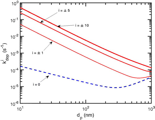
Table 1. Chamber parameters used for base-case simulations.

Variable	Value
ke	$0.1 {\mathrm{s}}^{-1}$
R	1.43 m
ρp	1.55 g cm^–3
g	9.807 m s^–2
η	$18.27\times {10}^{-6} \text{kg} {\mathrm{m}}^{-1} {\mathrm{s}}^{-1}$
kB	$1.381 {\mathrm{m}}^2 \text{kg} {\mathrm{s}}^{-2} {\mathrm{K}}^{-1}$
T	298.15 K
e	$1.602\times {10}^{-19} \mathrm{C}$
$\overline{E}$	$4500 \mathrm{V} {\mathrm{m}}^{-1}$
$k_{\text{iw}}$	$25\times {10}^{-3} {\mathrm{s}}^{-1}$
${\beta }^{\text{ir}}$	$1.6\times {10}^{-6} {\text{cm}}^3 {\mathrm{s}}^{-1}$
ϵ0	$8.854\times {10}^{-12} \mathrm{F} {\mathrm{m}}^{-1}$
${\mu }_{\text{ion}}^{+}$	$1.20\times {10}^{-4} {\mathrm{m}}^2 {\mathrm{V}}^{-1} {\mathrm{s}}^{-1}$
${\mu }_{\text{ion}}^{-}$	$1.35\times {10}^{-4} {\mathrm{m}}^2 {\mathrm{V}}^{-1} {\mathrm{s}}^{-1}$
q	$4 {\text{cm}}^{-3} {\mathrm{s}}^{-1}$

3.2. Dynamics of primary ions

The number of elementary charges is often estimated using parameterizations, for example, the Wiedensohler charge distribution approximation (Wiedensohler 1988). The charge fraction distribution, p_i, on an aerosol population is often assumed to be in steady state upon entry into the chamber or soon thereafter (Charan et al. 2018; López-Yglesias and Flagan 2013a). However, this “neutralizer steady state” requires that diffusion charging (both increasing and decreasing the charges on the particles) be the dominant process influencing the charge distribution. In neutralizers, this is achieved with a very high primary ion production rate. Yet, it is possible that a “neutralizer” steady-state charge distribution is not achieved in a chamber (Charan et al. 2018), resulting in an undercharged distribution. Primary ions are constantly produced in the atmosphere and in chambers due to background cosmic rays (Franchin et al. 2015; Kirkby et al. 2016; Wagner et al. 2017). Stable positive and negative ions interact with aerosol particles, and thus, change the aerosol population’s charge distribution. Because charged particles are deposited more readily to the chamber walls, and because the deposition rate competes with the diffusion charging rates, deposition also changes the charge distribution of the remaining particles. Here, as a simplification, we assume that the charge distribution does not influence coagulation (we are considering relatively large particles).

In this work, we use the term “primary ion” to describe the ensemble of small, stable cluster ions containing a molecular ion, some water molecules, and perhaps a few highly polar molecules. These will govern the subsequent diffusion charging of larger particles; they may or may not have a similar composition to corresponding atmospheric ions (for example, bisulfate dominates small anions during the day in the atmosphere, but will only appear in a chamber if sulfuric acid vapor is being produced, and base vapors such as ammonia may have very different concentrations in a chamber than in the atmosphere). We follow López-Yglesias and Flagan (2013a) and select single ion mobilities representative of atmospheric conditions. In reality, chambers and the atmosphere have (different) ion-mobility distributions, but this has only a minor quantitative effect on the conclusions we present here.

Primary ion pairs in the chamber are produced at a rate, q, whose units are cm⁻³s^–1. The primary ions are lost to the walls, due to recombination with other ions of opposite charges, and to aerosol particles. The balance equation is (3) $$\begin{array}{c}\frac{\mathrm{d}{C}^{\pm }}{\mathrm{d}t}=q-k_{\text{iw}}^{\pm }{C}^{\pm }-{\beta }^{\text{ir}}{C}^{\pm }{C}^{\mp }\hfill \\ -C^{\pm }{\int }_{d_p}\left(\sum _{i=-\infty }^{\infty }{\beta }_i^{\pm }(d_p)n(d_p)p_i(d_p)\right)\mathrm{d}{d}_p,\hfill \end{array}$$(3) where C is the number concentration of primary ions, $k_{\text{iw}}$ is the ion deposition rate coefficient to the wall, ${\beta }^{\text{ir}}$ is the ion recombination rate coefficient, and the last term on the right-hand side is the sink rate of primary ions on aerosol particles (Gonser et al. 2014; Hoppel and Frick 1986; Horrak et al. 2008). In the last term, β_i is the ion–aerosol attachment coefficient between ions and particles of charge i at size d_p; p_i is the fraction of aerosol particles with charge i as a function of size, d_p; and n is the particle size distribution function. For β_i, whose units are cm³s^–1, we use tabulated coefficients of López-Yglesias and Flagan (2013a, 2013b) to a power-law expansion of numerical solutions to the attachment coefficients. This is because the most up-to-date results are those of López-Yglesias and Flagan (2013a).

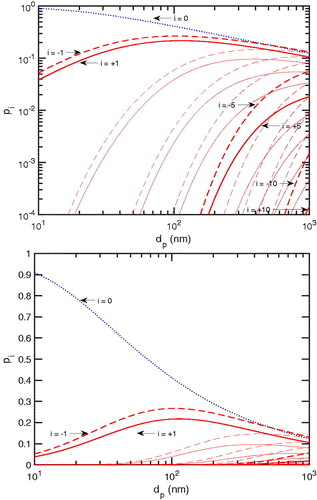
If the ion-pair formation rate, q, is great enough for the diffusion charging and neutralization rates to be much larger than any other rates affecting the number and charge balance of a particle population, $n(d_p),$ then the charge distribution $p_i(d_p)$ will reach the “neutralizer” steady state. This is a requirement for accurate measurement of number distributions using mobility classifiers (Charan et al. 2018). We show the neutralizer steady-state charge distribution for equal concentrations of primary cations and anions (as found in a neutralizer where primary ion recombination is the main primary ion sink) in Figure 2. Like before, to be accurate and consistent, we also use the updated power-law coefficients for the steady-state approximation—also provided by López-Yglesias and Flagan (2013a).

Figure 2. Charge fraction at the neutralizer steady state as a function of size in a logarithmic scale on top and linear scale bottom. The fraction of neutral particles, i = 0, is shown in dotted (blue) while those for charged particles, $\left|i\right|>0,$ are shown in solid (red) for positive charge and in dashed (red) negative charge. Most particles are neutral or singly charged when $d_p\le$ 100 nm.

4. Methods

Utilizing the Bridges system (Nystrom et al. 2015; Towns et al. 2014), we carry out numerical simulations to explore the effects of the primary ion balance on larger particles in an environmental chamber (roughly cubical teflon-film bag with 2.15 m long edges). We model the evolution of the concentrations of primary ions, C⁺ and C^–, as well as the aerosol size and charge distribution, $n(d_p)$ and $p_i(d_p),$ for different physical parameters of interest like the production rate and the average electric field in the chamber. We solve (3) to obtain values for C⁺ and C^–; similarly, we update p_i according to (4) $$\begin{array}{c}\frac{\mathrm{d}}{\mathrm{d}t}\left(n{p}_i\right)=C^{+}{\beta }_{i-1}^{+}\left(n{p}_{i-1}\right)+C^{-}{\beta }_{i+1}^{-}\left(n{p}_{i+1}\right)\hfill \\ \hspace{1em}-(C^{+}{\beta }_i^{+}+C^{-}{\beta }_i^{-})\left(n{p}_i\right).\hfill \end{array}$$(4)

We start with q = 4 cm^–3 s⁻¹, but we vary the primary ion formation rate between 2 and 20 cm^–3 s⁻¹. We initialize the chamber with the primary ion concentrations, $C^{+}=C^{-}=$ 1000 cm^–3, without any particles present. Unless stated otherwise, the values of the parameters involved in the simulations are listed in Table 1.

For these simulations, the particles initially have a lognormal particle distribution with a geometric mean of 100 nm and a standard deviation of 1.2. For the initial conditions, we considered three different total particle number concentrations: $N=\int n(d_p)\mathrm{d}{d}_p=2850,28500,285000$ cm⁻³. With a density of 1.55 g cm⁻³, this corresponds to a suspended seed mass concentration ranging from 3.74 to 374 μg m⁻³, which in turn generously spans the range typically used in seeded chamber experiments.

We consider two initial charge distributions, “neutral” and “charged.” Here, “neutral” means “uncharged” and corresponds to a case where the seed particles were generated by nucleation following flash vaporization of a low vapor-pressure oil. Also, “charged” means the “neutralizer steady state” condition and corresponds to a case where seed particles were formed via nebulization followed by passage through a high ionization rate neutralizer. We assume this spans the likely initial conditions in chamber experiments, though it is possible that an overcharged population of seeds could be produced by nebulization followed by inadequate neutralization.

Besides the diffusion of primary ions to the aerosol particles, we assume that the deposition of particles to chamber walls is the only process taking place inside the chamber according to the equation: (5) $$\frac{\partial \left(n(d_p)p_i(d_p)\right)}{\partial t}=g_{\text{dep}}^i(d_p),$$(5) where $g_{\text{dep}}^i(d_p)=-k_{\text{dep}}^i{p}_{i}n.$ We omit coagulation and condensation in order to focus exclusively on the role of diffusion charging on particle wall deposition. In summary, we solve (3(3) $$\begin{array}{c}\frac{\mathrm{d}{C}^{\pm }}{\mathrm{d}t}=q-k_{\text{iw}}^{\pm }{C}^{\pm }-{\beta }^{\text{ir}}{C}^{\pm }{C}^{\mp }\hfill \\ -C^{\pm }{\int }_{d_p}\left(\sum _{i=-\infty }^{\infty }{\beta }_i^{\pm }(d_p)n(d_p)p_i(d_p)\right)\mathrm{d}{d}_p,\hfill \end{array}$$(3) ), (4(4) $$\begin{array}{c}\frac{\mathrm{d}}{\mathrm{d}t}\left(n{p}_i\right)=C^{+}{\beta }_{i-1}^{+}\left(n{p}_{i-1}\right)+C^{-}{\beta }_{i+1}^{-}\left(n{p}_{i+1}\right)\hfill \\ \hspace{1em}-(C^{+}{\beta }_i^{+}+C^{-}{\beta }_i^{-})\left(n{p}_i\right).\hfill \end{array}$$(4) ), and (5(5) $$\frac{\partial \left(n(d_p)p_i(d_p)\right)}{\partial t}=g_{\text{dep}}^i(d_p),$$(5) ) to determine the concentration of primary ions, C, the charge fraction, p_i, and the particle size distribution, n, at each time step.

5. Results and discussion

5.1. Primary ion evolution

In Figure 3, we show the competing rates and the concentration of primary ions for the three different initial particle number concentrations. The particles start “charged” in this case, though this makes little difference to the overall behavior of primary ions within chamber experiments.

Figure 3. The evolution of primary ions. In the left plots, the competing rates of primary ions dynamics are shown: condensation sink, wall loss, recombination loss, and production. In the right plots, the corresponding concentrations of negative and positive primary ions are shown. In all cases, the production rate of primary ions is 4 cm^–3 s⁻¹ for each negative and positive ions, and thus 8 cm^–3 s⁻¹ in total, and the mean diameter of the condensation sink is 100 nm. The total number of aerosol particles in the condensation sink is 2850, 28,500, and 285,000 cm^–3 for the top, middle, and bottom plots, respectively. As the total number of particles increases from top to bottom, the higher and more prominent the condensation sink is compared to the competing rates of wall loss and recombination loss. The concentration of positive ions in the right plots is higher than the negative one because the mobility of negative ions is higher and so more negative ions diffuse to the particles.

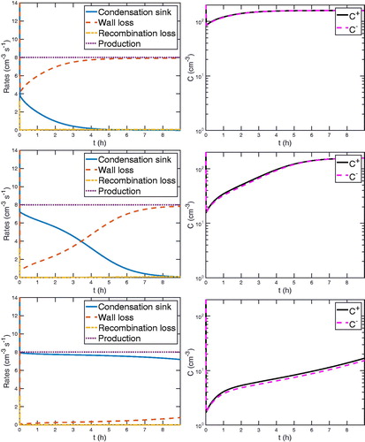
On the left, we plot the competing rates of primary ions dynamics: condensation sink, wall loss, and recombination loss. On the right, we plot the corresponding concentration of negative and positive primary ions. From the left column we see that recombination is negligible for these conditions, and even for the lowest seed concentration, diffusion charging (the condensation sink) competes with primary ion deposition (wall loss). In that one case, wall loss eventually becomes dominant as the total particle number drops over the course of the two hour simulation; in the higher condensation sink cases, primary ion wall loss ranges from small to negligible and diffusion charging is the dominant process balancing ion-pair formation, which reflects the dominance of the last term in (3(3) $$\begin{array}{c}\frac{\mathrm{d}{C}^{\pm }}{\mathrm{d}t}=q-k_{\text{iw}}^{\pm }{C}^{\pm }-{\beta }^{\text{ir}}{C}^{\pm }{C}^{\mp }\hfill \\ -C^{\pm }{\int }_{d_p}\left(\sum _{i=-\infty }^{\infty }{\beta }_i^{\pm }(d_p)n(d_p)p_i(d_p)\right)\mathrm{d}{d}_p,\hfill \end{array}$$(3) ).

On the right, we see that the primary ion concentration evolves significantly in all cases. Because we add a sink (diffusion charging) at t = 0, in all three simulations the ion concentrations at first drop rapidly until a chamber steady state is established including the diffusion charging. Positive ions are always slightly more abundant because of their lower mobility, but the charging rates are identical. In all cases, the primary ion concentrations evolve significantly over the course of the simulation; for example, in the middle case which is most typical of a seeded chamber experiment, the concentrations change by almost an order of magnitude. This suggests that we may well find a significant evolution of the particle wall losses driven by this diffusion charging over the course of an experiment.

5.2. Charge distribution evolution

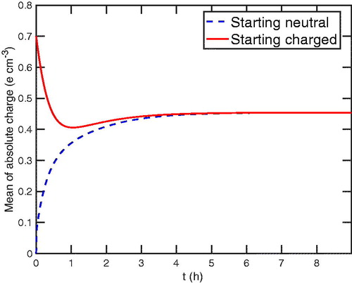
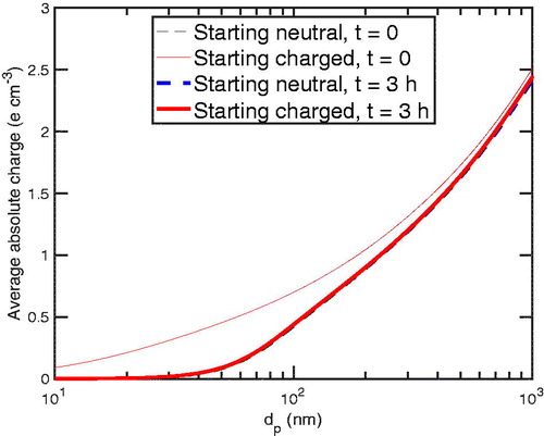
The evolving primary ion concentration suggests that the particle charge distribution, $p_i(d_p),$ will also evolve in time. Further, the initial condition, $p_i(d_p,t=0),$ is likely to matter. In Figure 4, we show the average absolute charge, $\sum _i\left|i\right|p_i,$ for particles of the modal size, $d_p=$ 100 nm, with the smallest value of total particle number concentration, N = 2850 cm^–3. The neutral initial condition is a dashed (blue) curve and the charged initial condition is a solid (red) curve. Both charge distributions converge to a new chamber steady-state charge distribution in approximately 3 h, which also corresponds to where the concentrations of primary ions reach a steady state in the top left plot in Figure 3.

Figure 4. The average absolute charge, $\sum _i\left|i\right|p_i,$ for $d_p=$ 100 nm as a function of time, t. Both the starting-neutral and starting-charged particles converge to a value that is lower than the original steady state in roughly 3 h, indicating the new chamber particle charge steady state.

The chamber steady state differs significantly from the steady state within a neutralizer, where diffusion charging completely dominates the charging and neutralization of particles. Here, while the charged particles are lost to the walls, depleting the particle charge state, the primary ions effectively try to reestablish the prescribed steady-state distribution. In Figure 5, we depict the chamber steady state by showing the average of the absolute charge for all particle sizes after 3 h and both initial conditions at t = 0, where the thinner (red) curve refers to the “charged” steady state found in a neutralizer. The average absolute charge on smaller particles, $d_p\mathrm{\lesssim }50 \text{nm},$ is much more depleted compared to the “neutralizer steady state” than on larger particles. This is because charged smaller particles are lost more readily to chamber walls as seen in Figure 1.

Figure 5. The average absolute charge as a function of size for t = 0 and t = 3 h. The depleted charge state is seen as the charged particles lose their average charge from t = 0 to t = 3 h.

5.2.1. Particle wall loss evolution

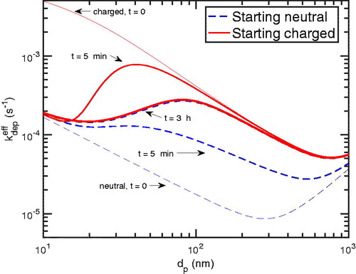
In Figure 6, we show the effective deposition rate coefficient as a function of particle size, as per (2). We show the initial values for the starting-charged and starting-neutral distributions, which bound the values; between them are the effective coefficients as they evolve in time. As with the mean absolute charge in Figure 4, the effective coefficients decrease in time for initially charged particles and increase in time for initially neutral particles. They converge in roughly 3 h on the chamber steady state. For these conditions, most of the deposition coefficients change by up to an order of magnitude over time, suggesting that this may play a significant role in chamber experiments. It is important to note, however, that the chamber steady state is not stationary; rather, it continues to evolve as a result of the continuous diffusion charging and the changing particle size distribution within the chamber. We probe this effect next.

Figure 6. The effective deposition rate coefficient at different times for the starting-charged and starting-neutral particles. For the starting-charged particles, the effect of the charge depletion can be seen as the effective coefficient is reduced. For the starting-neutral ones, the effective coefficient is enhanced as more particles gain charge. The two converge after approximately 3 h, consistent with Figures 4 and 5.

5.3. Effect of the total particle number

As we showed in Figure 3, the condensation sink—the last term in (3)—has a greater effect on the primary ion balance as the total particle number increases. The absolute rate of particle deposition should increase as the total particle number increases due to the first-order dependence shown in (1); however, to the extent that particle loss is controlled by diffusion charging and thus ultimately the ion-pair formation rate, q, the total particle deposition rate could be effectively constant and thus zeroth order.

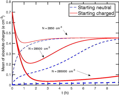
In Figure 7, we show the average charge vs in time at $d_p=$ 100 nm. The time to achieve the chamber steady-state charge distribution increases as the number increases. Moreover, the average absolute charge decreases as the total particle number increases. This is because the more particles there are, the higher the rate of particle deposition to the walls—but, instead of having a more robust effect of primary ions, their effect is diminished relative to the deposition rate because as the number of particle increase, it takes longer to effectively change the particle charge state. This is especially true for the smallest particles; however, for the largest total number, particles of all sizes are significantly depleted in charge, even after 8 h.

Figure 7. The average absolute charge of particles with $d_p=$ 100 nm for different total particle numbers in the condensation sink. As the total particle number increases, the more the charge is depleted.

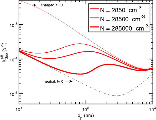
Finally, the total particle number influences the effective particle deposition because it influences the charge distribution. In Figure 8, we show the effective deposition rate coefficients at 3 h for the starting-charged (that is, with a “neutralizer steady state”) cases. As the total particle number increases, the effective coefficient decreases due to the depletion of charge on particles. The effective deposition coefficient will continue to decrease until the chamber steady state is achieved and then it will reverse course and slowly increase with decreasing particle number. Notably, when the total number is largest in Figure 8, the effective deposition rate coefficient follows the neutral coefficient in the limit of smaller particles and the charged one in the limit of larger particles.

Figure 8. The effective deposition rate after 3 h for different total particle concentrations. The charge depletion is reflected in the lower coefficient for higher concentrations.

5.4. Effect of the of primary ion production rate

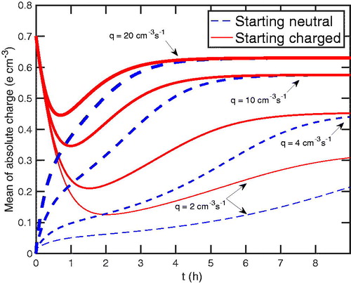
The primary ion production rate will directly affect the chamber steady-state charge distribution; the charge distribution is depleted under the conditions we have modeled, and so we expect it to rise toward the neutralizer steady state (initially charged) distribution at a sufficiently high primary ion production rate. We study this effect for N = 28,500 cm^–3, which is most typical of seeded chamber experiments. As the production rate is increased from $q=$ 2 to 20 cm^–3s^–1, the diffusion charging of particles increases as well. In Figure 9, we show the average absolute charge vs in time at $d_p=$ 100 nm for varying production rates, q. The value of the production rate is indicated by curve thickness: the thicker, the higher. We note that as the production is increased, the shorter time is required to achieve a higher chamber charge steady state.

Figure 9. The mean of absolute charge as a function of time for different production rates, $q=$ 2, 4, 10, 20 cm^–3s^–1. The dashed (blue) curves represent particles that started uncharged or neutral; the solid (red) particles that started as charged at the neutralizer steady state. The thicker the curve, the more the production rate. We note that the higher the production rate of primary ions, the higher the achieved chamber charge steady-state. Moreover, the higher the production rate, the faster this steady-state is achieved.

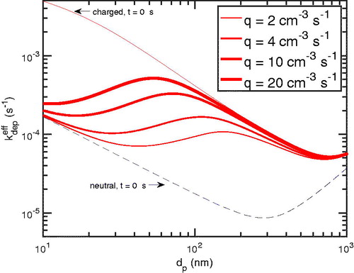
The effective deposition rate coefficient also increases as the production rate is increased. This can be seen in Figure 10. For smaller particles ($d_p\mathrm{\lesssim }$ 100 nm) the effect is almost linear—the effective deposition coefficient nearly doubles as the primary ion production rate doubles. This indicates a nearly zeroth order particle loss for these smaller particles.

Figure 10. The effective deposition rate coefficient for varying production rates of primary ions, q, after 3 h. The effective coefficient is increased due to the increase of the production rate of primary ions.

5.5. Effect of the electric field

Particle charging only influences particle losses when there is an electric field near the chamber surface. The length scale is small, as for typical conditions turbulent transport carries particles to within 1 mm of the wall, and so fluctuations in the surface charge density on this length scale will influence the field above the wall even for a chamber that is free of static charge overall. Of course, in conducting chambers with controlled electric fields, for example, CLOUD chamber (Kirkby et al. 2016), the field can be large and constant. It is the average of the absolute value of the field within the nominally laminar boundary layer, $\overline{E},$ that we care about.

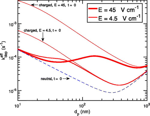
Figure 11 shows the effective deposition rate coefficient profiles for both values of the electric field. We see that even with the lesser field, the coefficient varies by five-fold for particles less than $d_p=$ 100 nm. In both cases the deposition deviates significantly from the neutral deposition, which is the limit for either an uncharged particle distribution or a zero-field chamber. For a chamber constructed with insulating materials, there is a minimum average field due to thermal fluctuations in the charge density even at equilibrium, whereas for a conducting chamber with very careful management of any surfaces that might sustain a static charge the zero-field limit is possible.

Figure 11. The effective deposition rate coefficient after 3 h for two different values of the electric field near the chamber surface, $\overline{E}.$ The effective coefficient is decreased due to the decrease in the electrostatic deposition velocity of particles.

5.6. Including coagulation dynamics

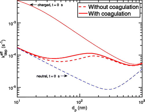
We conducted these simulations considering only particle charging and deposition in order to isolate these effects. However, for the sake of completeness, we show the effect of including particle coagulation in Figure 12 after 3 h. We follow the coagulation formulation of Seinfeld and Pandis (2016) without considering the effect of charges. Here, along with particle deposition and primary ions dynamics, we added coagulation dynamics for the the largest total particle number 285,000 cm^–3, where coagulation is most significant. While coagulation significantly influences the size distribution, decreasing the total number and increasing the diameter mean, the maximal influence on the deposition rate coefficient profile or the particle charge distribution is roughly 20%.

Figure 12. Including coagulation along particle deposition and primary ions dynamics. The deposition rate coefficient after 3 h profile is not changed significantly when considered coagulation (solid) besides deposition and primary ions (dashed).

6. Measurement of particle wall losses

To test our model of charging and particle wall loss, we analyze a wall-loss calibration experiment first reported by Wang et al. (2018). In this experiment, the CMU chamber is cleaned and then filled with ammonium sulfate seeds with a modal diameter near 100 nm and an initial concentration of 28,500 cm^–3. The chamber is a roughly cubical teflon-film bag with 2.15 m long edges. The seeds are formed from a nebulized aqueous solution and passed through a diffusion drier and a neutralizer before entering the chamber, held at roughly 5% RH. The distribution is then measured using a scanning mobility particle sizer (SMPS, TSI Inc.) over the next 8 h.

In order to reduce noise associated with differencing data, we fit the raw distributions for each SMPS scan to a tailing Gaussian function. The function reproduces the number, surface area and volume distributions with high fidelity and without bias. We then smooth the time evolution of the total number and scale the amplitude of each fitted distribution by the ratio $a(t)=\tilde{N}/N$ to give the best estimate of the time dependence of the number distribution ${\tilde{n}}_N^{°}(t),$

With the distributions fitted and smoothed, we find the rate of change of the particle size distribution, corrected for coagulation and ventilation, and then estimate a pseudo first-order deposition coefficient $k^I(d_p)$ based on the residual observed loss rates. (6) $$\frac{d}{dt}{\tilde{n}}_N^{°}(d_p)=R_{\text{coag}}(d_p)+R_{\text{vent}}(d_p)-k^I(d_p){\tilde{n}}_N^{°}(d_p)$$(6)

For all of these calculations, we calculate uncertainty from the confidence intervals of the two distributions, added in quadrature.

In Figure 13, we show the integrated rate, $d\tilde{\mathcal{N}}/dt.$ This shows an overall loss of a bit less than 1 s^–1, dropping slowly as the total number declines as well. These integrated number loss rates are notably similar to typical ion-pair formation rates of 2 cm^–3 s⁻¹ reported by Kirkby et al. (2016), which suggests that particle charging plays a major role in the overall particle deposition. 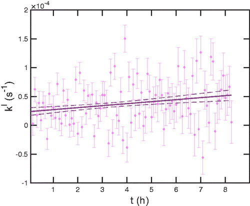In Figure 14, we show the time evolution of the pseudo-first order deposition coefficients, $k^I(d_p,t),$ for particles near the volume mode. This is representative; all of the pseudo first-order deposition coefficients increase with time. To capture this, we perform linear fits in time at each size; the fits, with 68% confidence intervals, yield our final best estimate of $k^I(d_p,t).$

Figure 13. Total particle loss rates over time, based on fitted and smoothed size distributions for successive scans, s: ($\tilde{\mathcal{N}}(t_{s+1})-\tilde{\mathcal{N}}(t_s))/(t_{s+1}-t_s).$

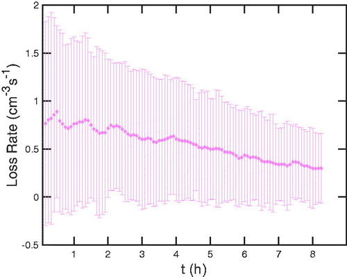
Figure 14. Pseudo-first order deposition coefficient for 168.2 nm particles over time. Points are the size-resolved number differences with error, while the line is an uncertainty weighted linear fit, with 68% confidence intervals as dashed curves.

In Figure 15, we show $k^I(d_p)$ obtained from those linear fits at four selected times spanning the experiment. We superimpose model results for the corresponding times of particle that started neutral with $\overline{E}=$ 30 V/cm and $q=$ 1 cm^–3s^–1. The figure also shows loss constants for sulfuric acid (red) and a series of SVOCs (green) obtained and reported earlier with similar chamber operating conditions (Ye et al. 2016). The vapor losses constrain the chamber turbulence frequency, k_e, and so the neutral deposition coefficient, which we show with a dashed blue curve over the size range measured by the SMPS. In dashed red, we show the effective wall loss coefficient for particles at the neutralizer steady state charge distribution.

Figure 15. Evolution of the size-dependent pseudo first-order deposition coefficients, showing values at the beginning, one-third, two-thirds and at the end of the wall-loss experiment. The red and green circles are vapor loss constants for sulfuric acid and organics, and the dashed blue curve is a size-dependent curve for particle deposition based on the k_e turbulence value given by those vapor loss coefficients. The dashed red curve corresponds to the particles at the neutralizer charge steady state with $\overline{E}=$ 30 V/cm and $q=$ 1 cm^–3s^–1.

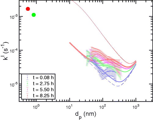
Based on the increasing pseudo first order deposition coefficients, we conclude that in this experiment the seed particles entered the chamber undercharged, most notably near the number mode at 100 nm. Over the next several hours the charge distribution likely grew toward the chamber steady state discussed above. However, the correspondence between the measured and modeled deposition coefficients is modest, and the relative paucity of measured parameters makes the model under constrained. Specifically, k_e is not directly estimated by measuring vapor wall loss during these experiments, but rather we show values for similar conditions obtained several years earlier. Further, the actual charge distribution or even the particle mobility distribution (without passing sampled particles through a neutralizer) are not measured and the ion-pair formation rate is also unknown. Finally, the average absolute value of the electric field in the chamber is not measured, and, as discussed, the relevant property is this value very close to the walls (1 mm or less). Thus, while the results are consistent with an increasing particle charge distribution over time, a full model-measurement comparison will require a more complete set of experimental constraints.

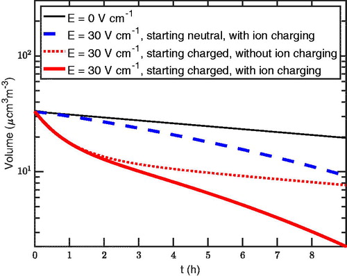
Finally, in Figure 16, we show the total volume of particles inside the chamber as a function in time. For this, we only consider particle wall loss to show the effect of taking into account different processes on the amount of loss for a typical chamber experiment. We see a clear decrease of the volume between the case of no electric field (black) and the cases with an electric field present (red and blue). Further, while both decrease similarly in the present of primary ion charging, the volume loss of charged particles is higher due to the presence of the electric field. In the case where there is no ion charging (dashed red), we see the loss is lesser than the equivalent loss with primary ion charging (continuous red).

Figure 16. The total volume of particles inside the chamber with only wall loss taken into account. The solid thin (black) curve corresponds to the case without an electric field present. The dashed (blue) curve corresponds to the case with an electric field of $\overline{E}=$ 30 V/cm and the particles starting all neutral, allowing primary ion charging with $q=$ 1 cm^–3s^–1. The solid thick (red) curves correspond to the case with an electric field of $\overline{E}=$ 30 V/cm and the particles starting in the neutralizer steady state or charged. The dotted (red) curve is for the case without primary ion charging and the continuous one with primary ion charging with $q=$ 1 cm^–3s^–1.

7. Conclusion

Primary ion formation and loss significantly influence suspended particle deposition (wall loss) in environmental chambers constructed from insulating material (i.e., Teflon). The effects are coupled, and the consequence is effective particle deposition that is not first order but rather intermediate between zeroth and first order, and that also evolves in time. The effects are most pronounced for particles smaller than 100 nm, where the suspended particle charge distribution is significantly depleted compared to the steady-state charge distribution found in a high ionization rate particle neutralizer. However, the effects span the full sub-micron range and depend on all of the relevant parameters: primary ion formation rate, average electric field near the chamber walls, the suspended particle concentration, and the initial particle size distribution. In many cases typical of chamber experiments, the effective wall loss coefficients evolve significantly for multiple hours. This strongly suggests that all of these quantities need to be measured, or in the very least controlled, in order to avoid uncontrolled errors in analysis of chamber data.

Declaration of interest statement

We declare no financial conflict of interest.

Correction Statement

This article has been republished with minor changes. These changes do not impact the academic content of the article.

Additional information

Funding

This work was supported by the National Science Foundation under Grant AGS1740665. This work used the Extreme Science and Engineering Discovery Environment (XSEDE), which is supported by National Science Foundation grant number ACI-1548562. Specifically, it used the Bridges system, which is supported by NSF award number ACI-1445606, at the Pittsburgh Supercomputing Center (PSC). We simulated a wide array of parameters relevant to this physical system, but only used part of the data generated that was most representative of the overall behavior.

References

- Charan, S. M., W. Kong, R. C. Flagan, and J. H. Seinfeld. 2018. Effect of particle charge on aerosol dynamics in Teflon environmental chambers. Aerosol Sci. Technol. 52 (8):854–71. doi:10.1080/02786826.2018.1474167.
- Crump, J. G., R. C. Flagan, and J. H. Seinfeld. 1982. Particle wall loss rates in vessels. Aerosol Sci. Technol. 2 (3):303–9. doi:10.1080/02786828308958636.
- Crump, J. G., and J. H. Seinfeld. 1981. Turbulent deposition and gravitational sedimentation of an aerosol in a vessel of arbitrary shape. J. Aerosol Sci. 12 (5):405–15. doi:10.1016/0021-8502(81)90036-7.
- Franchin, A., S. Ehrhart, J. Leppä, T. Nieminen, S. Gagné, S. Schobesberger, D. Wimmer, J. Duplissy, F. Riccobono, E. M. Dunne, et al. 2015. Experimental investigation of ion–ion recombination under atmospheric conditions. Atmos. Chem. Phys. 15 (13):7203–16. doi:10.5194/acp-15-7203-2015.
- Gonser, S. G., F. Klein, W. Birmili, J. Größ, M. Kulmala, H. E. Manninen, A. Wiedensohler, and A. Held. 2014. Ion–particle interactions during particle formation and growth at a coniferous forest site in central Europe. Atmos. Chem. Phys. 14 (19):10547–63. doi:10.5194/acp-14-10547-2014.
- Hoppel, W. A., and G. M. Frick. 1986. Ion—aerosol attachment coefficients and the steady-state charge distribution on aerosols in a bipolar ion environment. Aerosol Sci. Technol. 5 (1):1–21. doi:10.1080/02786828608959073.
- Horrak, U., P. P. Aalto, J. Salm, K. Komsaare, H. Tammet, J. M. Mäkelä, L. Laakso, and M. Kulmala. 2008. Variation and balance of positive air ion concentrations in a boreal forest. Atmos. Chem. Phys. 8 (3):655–75. doi:10.5194/acp-8-655-2008.
- Kirkby, J., J. Duplissy, K. Sengupta, C. Frege, H. Gordon, C. Williamson, M. Heinritzi, M. Simon, C. Yan, J. Almeida, et al. 2016. Ion-induced nucleation of pure biogenic particles. Nature 533 (7604):521–6. doi:10.1038/nature17953.
- Krechmer, J. E., D. Pagonis, P. J. Ziemann, and J. L. Jimenez. 2016. Quantification of gas-wall partitioning in Teflon environmental chambers using rapid bursts of low-volatility oxidized species generated in situ. Environ. Sci. Technol. 50 (11):5757–65. doi:10.1021/acs.est.6b00606.
- López-Yglesias, X., and R. C. Flagan. 2013a. Ion–aerosol flux coefficients and the steady-state charge distribution of aerosols in a bipolar ion environment. Aerosol Sci. Technol. 47 (6):688–704. doi:10.1080/02786826.2013.783684.
- López-Yglesias, X., and R. C. Flagan. 2013b. Population balances of micron-sized aerosols in a bipolar ion environment. Aerosol Sci. Technol. 47 (6):681–7.
- Matsunaga, A., and P. J. Ziemann. 2010. Gas-wall partitioning of organic compounds in a Teflon film chamber and potential effects on reaction product and aerosol yield measurements. Aerosol Sci. Technol. 44 (10):881–92. doi:10.1080/02786826.2010.501044.
- McMurry, P. H., and D. Grosjean. 1985. Gas and aerosol wall losses in Teflon film smog chambers. Environ. Sci. Technol. 19 (12):1176–82. doi:10.1021/es00142a006.
- McMurry, P. H., and D. J. Rader. 1985. Aerosol wall losses in electrically charged chambers. Aerosol Sci. Technol. 4 (3):249–68. doi:10.1080/02786828508959054.
- Nystrom, N. A., M. J. Levine, Z. Roskies, and J. Scott. 2015. Bridges: A uniquely flexible HPC resource for new communities and data analytics. In Proceedings of the 2015 XSEDE Conference: Scientific Advancements Enabled by Enhanced Cyberinfrastructure, 30, ACM. July 2015, St. Louis Missouri. doi:10.1145/2792745.2792775.
- Pierce, J. R., G. J. Engelhart, L. Hildebrandt, E. A. Weitkamp, R. K. Pathak, N. M. Donahue, A. L. Robinson, P. J. Adams, and S. N. Pandis. 2008. Constraining particle evolution from wall losses, coagulation, and condensation-evaporation in smog-chamber experiments: Optimal estimation based on size distribution measurements. Aerosol Sci. Technol. 42 (12):1001–15. doi:10.1080/02786820802389251.
- Sakamoto, K. M., J. R. Laing, R. G. Stevens, D. A. Jaffe, and J. R. Pierce. 2016. The evolution of biomass-burning aerosol size distributions due to coagulation: Dependence on fire and meteorological details and parameterization. Atmos. Chem. Phys. 16 (12):7709–24. doi:10.5194/acp-16-7709-2016.
- Schwantes, R. H., R. C. McVay, X. Zhang, M. M. Coggon, H. Lignell, R. C. Flagan, P. O. Wennberg, and J. H. Seinfeld. 2017. Science of the environmental chamber. In Advances in atmospheric chemistry, edited by J. R. Barker; A. L. Steiner; J. T. Wallington. 11th ed. 1–93. New Jersey: World Scientific.
- Seinfeld, J. H., and S. N. Pandis. 2016. Atmospheric chemistry and physics: From air pollution to climate change. Hoboken, New Jersey: John Wiley & Sons.
- Sunol, A. M., S. M. Charan, and J. H. Seinfeld. 2018. Computational simulation of the dynamics of secondary organic aerosol formation in an environmental chamber. Aerosol Sci. Technol. 52 (4):470–82. doi:10.1080/02786826.2018.1427209.
- Towns, J., T. Cockerill, M. Dahan, I. Foster, K. Gaither, A. Grimshaw, V. Hazlewood, S. Lathrop, D. Lifka, G. D. Peterson, et al. 2014. XSEDE: Accelerating scientific discovery. Comput. Sci. Eng. 16 (5):62–74. doi:10.1109/MCSE.2014.80.
- Trump, E. R., S. A. Epstein, I. Riipinen, and N. M. Donahue. 2016. Wall effects in smog chamber experiments: A model study. Aerosol Sci. Technol. 50 (11):1180–200. doi:10.1080/02786826.2016.1232858.
- Wagner, R., C. Yan, K. Lehtipalo, J. Duplissy, T. Nieminen, J. Kangasluoma, L. R. Ahonen, L. Dada, J. Kontkanen, H. E. Manninen, et al. 2017. The role of ions in new particle formation in the CLOUD chamber. Atmos. Chem. Phys. 17 (24):15181–97. doi:10.5194/acp-17-15181-2017.
- Wang, N., S. D. Jorga, J. R. Pierce, N. M. Donahue, and S. N. Pandis. 2018. Particle wall-loss correction methods in smog chamber experiments. Atmos. Meas. Tech. 11 (12):6577–88. doi:10.5194/amt-11-6577-2018.
- Wiedensohler, A. 1988. An approximation of the bipolar charge distribution for particles in the submicron size range. J. Aerosol Sci. 19 (3):387–9. doi:10.1016/0021-8502(88)90278-9.
- Ye, P., X. Ding, J. Hakala, V. Hofbauer, E. S. Robinson, and N. M. Donahue. 2016. Vapor wall loss of semi-volatile organic compounds in a Teflon chamber. Aerosol Sci. Technol. 50 (8):822–34. doi:10.1080/02786826.2016.1195905.
- Zhang, X., R. H. Schwantes, R. C. McVay, H. Lignell, M. M. Coggon, R. C. Flagan, and J. H. Seinfeld. 2015. Vapor wall deposition in Teflon chambers. Atmos. Chem. Phys. 15 (8):4197–214. doi:10.5194/acp-15-4197-2015.