Assessment and validation of a hygroscopic growth model with different water activity estimation methods

Abstract

Hygroscopic growth models are currently of interest as aids for targeting the deposition of inhaled drug particles in preferred areas of the lung that will maximize their pharmaceutical effect. Mathematical models derived to estimate hygroscopic growth over time have been previously developed but have not been thoroughly validated. For this study, model validation involved a comparison of modeled values to measured values when the growing droplet had reached equilibrium. A second validation process utilized a novel system to measure the growth of a droplet on a microscope coverslip relative to modeled values when the droplet is undergoing the initial rapid growth phase. Various methods currently used to estimate the water activity of the growing droplet, which influences the droplet growth rate, were also compared. Results indicated that a form of the hygroscopic growth model that utilizes coupled-differential equations to estimate droplet diameter and temperature over time was valid throughout droplet growth until it reached its equilibrium size. Accuracy was enhanced with the use of a polynomial expression to estimate water activity relative to the use of a simplified estimate of water activity based on Raoult’s Law. Model accuracy was also improved when constraining the film of salt solution surrounding the dissolving salt core at saturation.

Copyright © 2020 American Association for Aerosol Research

EDITOR:

• Nicole Riemer

1. Introduction

Interest in the properties and behavior of hygroscopic particles in the atmosphere has been ongoing for decades. For example, the physics and chemistry associated with cloud droplet formation have been studied extensively with the text by Pruppacher and Klett (2010) serving as an excellent summary of that complicated process. Similarly, the process by which inhaled hygroscopic particles deposit in the lung after transforming into a droplet is of interest in the health sciences. Some of the early work related to the development of a hygroscopic growth model was conducted by Ferron and his collaborators (Ferron 1977; Ferron, Kreyling, and Haider 1988) as an enhancement to the particle deposition model developed by the International Commission on Radiological Protection (ICRP) Task Group on Lung Dynamics (Bates et al. 1966). Currently, advancements in the use of computational fluid dynamics (CFD) modeling to simulate the deposition of drug/toxicant particles in the human lung include hygroscopic particle growth to, for example, enhance efforts to target the deposition sites of therapeutic pharmaceuticals (Longest and Hindle 2011; Feng et al. 2016).

The travel time for an inhaled particle to reach the first respiratory bifurcation is ∼0.2 s under normal breathing conditions (Longest, McLeskey, and Hindle 2010). The timescale within which the hygroscopic growth of a particle can occur in the lung is therefore very short and can be less than the time needed for hygroscopic particles to reach an equilibrium size. As a consequence, the accuracy of a hygroscopic growth model during the transient initial growth phase is of significant importance to lung deposition modelers. However, the validation of growth models during this phase is absent in the scientific literature, nor is there an adequate discussion of the role deliquescence plays in the initial growth of a particle over time. Furthermore, the influence of the method used to estimate water activity, a fundamental aspect of the hygroscopic growth model, on modeled droplet growth has not been previously evaluated. The hygroscopic growth of a pure NaCl (“salt”) aerosol will be used here to demonstrate these points because its properties are well known; it is expected to demonstrate significant growth that will aid in validating the hygroscopic growth model, and it has been used extensively as a model system for sea-salt aerosols (Hemminger 1999). As such this article will focus on the hygroscopic growth of an initially dry particle and not include initially liquid droplets that may subsequently undergo hygroscopic growth.

1.1. Deliquescence and hygroscopic growth

Deliquescence and hygroscopic growth are considered separate phenomena but necessarily have overlapping characteristics (Martin 2000). An accepted definition of deliquescence is the phase change from a dry particle to form an aqueous solution droplet at a threshold relative humidity, $\mathrm{RH}=\mathrm{ }{\mathrm{RH}}_0,$ below which this process cannot occur (Martin 2000; Cruz and Pandis 2000) (here we distinguish between a dry hygroscopic aerosol as a “particle” and a wet salt solution aerosol as a “droplet”). At ${\mathrm{RH}}_0,$ the atmosphere exhibits a water vapor pressure high enough to cause an imbalance in the thermodynamics of the salt–vapor system that initiates salt particle dissolution (Ewing 2005; Djikaev et al. 2001). However, this phase change necessarily involves growth relative to that of the original dry particle as water vapor condenses on the particle to ultimately form a saturated aqueous solution droplet (Ewing 2005). The resulting droplet size, when the droplet salt solution is at saturation, can be determined numerically if the ratio of the salt mass to water mass of the saturated solution is known. For example, the maximum solubility of NaCl is 36.3 g/100 g of H₂O at 37 °C (internal human body temperature). This equates to a mass percent of salt in the solution,$\mathrm{ }Y,$ of 26.6. Assuming the salt particle is a sphere, $Y$ can be expressed as a percentage value in terms of the diameter of the droplet,$\mathrm{ }\varphi ,$ and the diameter of the original salt particle, ${\varphi }_{\mathrm{p}},$ as: (1) $$Y\mathrm{ }=\frac{{\varphi }_{\mathrm{p}}^3{\rho }_{\mathrm{s}}}{\left({\varphi }^3-{\varphi }_{\mathrm{p}}^3\right){\rho }_w+{\varphi }_{\mathrm{p}}^3{\rho }_{\mathrm{s}}}100,$$(1) where ${\rho }_{\mathrm{s}}$ is the density of NaCl (2165 kg/m³) and ${\rho }_{\mathrm{w}}$ is the density of water (997 kg/m³). Solving Equation (1)(1) $$Y\mathrm{ }=\frac{{\varphi }_{\mathrm{p}}^3{\rho }_{\mathrm{s}}}{\left({\varphi }^3-{\varphi }_{\mathrm{p}}^3\right){\rho }_w+{\varphi }_{\mathrm{p}}^3{\rho }_{\mathrm{s}}}100,$$(1) for droplet size as a function of the original salt particle size results in (2) $$\varphi ={\varphi }_{\mathrm{p}}{\left[\frac{{\rho }_{\mathrm{s}}}{{\rho }_{\mathrm{w}}}\left(\frac{1}{Y/100}-1\right)+1\right]}^{1/3},$$(2) which reduces to $\varphi ={1.910\varphi }_{\mathrm{p}}$ for NaCl.

Deliquescence of a NaCl particle, therefore, results in a droplet with a completely dissolved core that is almost twice the size of the original dry particle. At ${\mathrm{RH}}_0$ the vapor pressure at the surface of the droplet solution,$\mathrm{ }{p}_{\mathrm{s},\mathrm{d}},$ is assumed to be at saturation and in equilibrium with the vapor pressure exerted by the water vapor in the atmosphere,$\mathrm{ }{p}_{\mathrm{v},\mathrm{a}}.$ A high-concentration salt solution exerts a lower vapor pressure than a more dilute solution (Hinds 1999). Therefore, ${\mathrm{RH}}_0$ is the relative humidity that results in the most concentrated (at solution saturation) and smallest fully dissolved salt solution droplet.

Prior research has determined ${\mathrm{RH}}_0$ for various water-soluble salts as well as the subsequent equilibrium size of the salt solution droplet as RH is increased above ${\mathrm{RH}}_0\mathrm{ }$(Tang, Munkelwitz, and Davis 1977; Russell and Ming 2002; Cruz and Pandis 2000). For example, Tang, Munkelwitz, and Davis (1977) observed an ${\mathrm{RH}}_0$ = 75.7% for pure NaCl in water at 25 °C. However, studies have shown that ${\mathrm{RH}}_0$ for NaCl is not constant for all conditions, for example ${\mathrm{RH}}_0$ is lowered for multi-component NaCl mixtures (Marcolli and Krieger 2006; Mauer and Taylor 2010) and higher temperatures (Tang and Munkelwitz 1993), whereas ${\mathrm{RH}}_0$ is raised for extremely small (<100 nm) NaCl particles (Russell and Ming 2002).

Experimental methods applied to determine ${\mathrm{RH}}_0$ and subsequent growth beyond the minimum droplet size at ${\mathrm{RH}}_0$ frequently involved the use of a tandem differential mobility analyzer (TDMA) consisting of two DMA’s in series to both produce a monodisperse aerosol and measure the droplet size distribution exiting a humid atmosphere while RH was slowly increased from ${\mathrm{RH}}_0$ (Li, Montassier, and Hopke 1992; Rader and McMurry 1986; Cruz and Pandis 2000; Tang, Munkelwitz, and Davis 1977). Because these experiments were typically performed with submicron particles (∼100–500 nm) and the residence time through the second DMA is longer than required for particles of that size to reach equilibrium, results obtained were those associated with the equilibrium droplet size and therefore commonly presented as a plot of growth factors of an initial dry particle diameter relative to RH.

Further growth of the saturated droplet when RH is increased beyond ${\mathrm{RH}}_0$ is the process that Martin (2000) refers to as “hygroscopic growth,” which is considered distinct from the growth that necessarily occurs during deliquescence. However, when inhaling a dry hygroscopic particle into the lung where $\mathrm{RH}$ approaches 99.5% (Asgharian 2004), the particle suddenly enters an environment where RH > ${\mathrm{RH}}_0.$ This sudden immersion into a high humidity environment results in a two-stage process (Cruz and Pandis 2000; Mauer and Taylor 2010; Van Campen, Amidon, and Zografi 1983) involving both core dissolution and subsequent droplet growth. 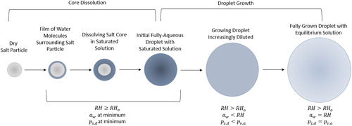During this process, the vapor pressure at the surface of the diluting droplet increases to match that of the atmosphere until $p_{\mathrm{s},\mathrm{d}}=p_{\mathrm{v},\mathrm{a}}$ resulting in an equilibrium droplet diameter as conceptualized in Figure 1.

Figure 1. Stages of hygroscopic growth of a dry salt particle. The ambient relative humidity, $\mathrm{RH},$ the water activity of the droplet solution, $a_{\mathrm{w}},$ and the vapor pressure exerted by droplet solution, $p_{\mathrm{s},\mathrm{d}},$ are given in relationship to the minimum $\mathrm{RH},$ ${\mathrm{RH}}_0,$ to achieve deliquescence and the vapor pressure exerted by water vapor in the atmosphere, $p_{\mathrm{v},\mathrm{a}}.$ Adapted from Mauer and Taylor (2010), and Van Campen, Amidon, and Zografi (1983).

1.2. Hygroscopic growth model development

Numerous papers and texts have described the development of a mathematical model to estimate the growth of hygroscopic compounds over time (Broday and Georgopoulos 2001; Ferron 1977; Ferron, Kreyling, and Haider 1988; Hinds 1999; Longest and Hindle 2011; Pruppacher and Klett 2010; Van Campen, Amidon, and Zografi 1983; Winkler-Heil, Ferron, and Hofmann 2014; Finlay 2001). The growth model has been developed in terms of both droplet mass and droplet diameter. In terms of droplet diameter, $\varphi ,$ the growth model can be expressed as (Broday and Georgopoulos 2001) (3) $$\frac{d\varphi }{dt}=\frac{4D_{\mathrm{v}}^{\mathrm{*}}{M}_{\mathrm{w}}}{R{\rho }_{\mathrm{d}}\varphi }\left[\frac{p_{\mathrm{v},\mathrm{a}}}{T_{\mathrm{a}}}-\frac{p_{\mathrm{s},\mathrm{d}}\left(T_{\mathrm{d}}\right)}{T_{\mathrm{d}}}\right],$$(3) where $D_{\mathrm{v}}^{\mathrm{*}}$ is the diffusivity of water vapor molecules modified to be applicable to both the continuum and non-continuum regimes, $M_{\mathrm{w}}$ is the molecular weight of water, $R$ is the universal gas constant, ${\rho }_{\mathrm{d}}$ is droplet density, $T_{\mathrm{a}}$ is ambient temperature, and $T_{\mathrm{d}}$ is droplet temperature. The density of a growing droplet is the density of a diluting salt solution with a constant mass of salt that can be expressed as (4) $${\rho }_{\mathrm{d}}=\frac{\left({\varphi }^3-{\varphi }_{\mathrm{p}}^3\right){\rho }_{\mathrm{w}}+{\varphi }_{\mathrm{p}}^3{\rho }_{\mathrm{s}}}{\left({\varphi }^3-{\varphi }_{\mathrm{p}}^3\right)+{\varphi }_{\mathrm{p}}^3}.$$(4)

Ambient RH, which, in fractional form, is equivalent to the environmental saturation ratio, $S_{\mathrm{R}},$ can be incorporated into the model given its association with $p_{\mathrm{v},\mathrm{a}}$ in Equation (3)(3) $$\frac{d\varphi }{dt}=\frac{4D_{\mathrm{v}}^{\mathrm{*}}{M}_{\mathrm{w}}}{R{\rho }_{\mathrm{d}}\varphi }\left[\frac{p_{\mathrm{v},\mathrm{a}}}{T_{\mathrm{a}}}-\frac{p_{\mathrm{s},\mathrm{d}}\left(T_{\mathrm{d}}\right)}{T_{\mathrm{d}}}\right],$$(3) (5) $$S_{\mathrm{R}}=\frac{\mathrm{RH}}{100}=\frac{p_{\mathrm{v},\mathrm{a}}}{p_{\mathrm{s},\mathrm{w}}\left(T_{\mathrm{a}}\right)},$$(5) where $p_{\mathrm{s},\mathrm{w}}$ is the saturation water vapor pressure over a flat surface for a given $T_{\mathrm{a}}.$

The computational form of the growth model must account for the effect of the curvature of the droplet, the droplet temperature, and its salt concentration on $p_{\mathrm{s},\mathrm{d}}(T_{\mathrm{d}})$ (Broday and Georgopoulos 2001). The effect of surface curvature was adjusted using the Kelvin equation. Likewise, the Clausius–Clapyron equation was used to determine the water vapor pressure at $T_{\mathrm{d}}$ relative to that at $T_{\mathrm{a}}$ to obtain an equation that relates $p_{\mathrm{s},\mathrm{d}}(T_{\mathrm{d}})$ as a function of the known value of $p_{\mathrm{s},\mathrm{w}}\left(T_{\mathrm{a}}\right)$ and water activity, $a_{\mathrm{w}},$ included to account for droplet salt concentration. In combined form these adjustments resulted in the following expression: (6) $$p_{\mathrm{s},\mathrm{d}}\left(T_{\mathrm{d}}\right)=p_{\mathrm{s},\mathrm{w}}\left(T_{\mathrm{a}}\right)a_{\mathrm{w}}\mathrm{e}\mathrm{xp}\left[\frac{4M_{\mathrm{w}}\sigma }{R{\rho }_{\mathrm{w}}\varphi T_{\mathrm{d}}}+\frac{h_{\mathrm{fg}}{M}_{\mathrm{w}}}{R}\left(\frac{1}{T_{\mathrm{a}}}-\frac{1}{T_{\mathrm{d}}}\right)\right].$$(6) An expanded form of Equation (3)(3) $$\frac{d\varphi }{dt}=\frac{4D_{\mathrm{v}}^{\mathrm{*}}{M}_{\mathrm{w}}}{R{\rho }_{\mathrm{d}}\varphi }\left[\frac{p_{\mathrm{v},\mathrm{a}}}{T_{\mathrm{a}}}-\frac{p_{\mathrm{s},\mathrm{d}}\left(T_{\mathrm{d}}\right)}{T_{\mathrm{d}}}\right],$$(3) is therefore (7) $$\frac{d\varphi }{dt}=\frac{4D_{\mathrm{v}}^{\mathrm{*}}{M}_{\mathrm{w}}{p}_{\mathrm{s},\mathrm{w}}\left(T_{\mathrm{a}}\right)}{R{\rho }_{\mathrm{d}}\varphi }\left[\frac{S_{\mathrm{R}}}{T_{\mathrm{a}}}-\frac{a_{\mathrm{w}}}{T_{\mathrm{d}}}\mathrm{e}\mathrm{xp}\left[\frac{4M_{\mathrm{w}}\sigma }{R{\rho }_{\mathrm{w}}\varphi T_{\mathrm{d}}}+\frac{h_{\mathrm{fg}}{M}_{\mathrm{w}}}{R}\left(\frac{1}{T_{\mathrm{a}}}-\frac{1}{T_{\mathrm{d}}}\right)\right]\right].$$(7)

The molecular diffusivity of water vapor modified for gas kinetic effects, $D_{\mathrm{v}}^{\mathrm{*}},$ can be calculated as follows (Pruppacher and Klett 2010; Broday and Georgopoulos 2001): (8) $$D_{\mathrm{v}}^{\mathrm{*}}=D_{\mathrm{v}}{\left[\frac{1}{1+2{\delta }_{\mathrm{c}}\lambda /\varphi }+\frac{2D_{\mathrm{v}}}{\varphi {\alpha }_{\mathrm{c}}\sqrt{R{T}_{\mathrm{a}}/2\pi M_{\mathrm{w}}}}\right]}^{-1},$$(8) where $D_{\mathrm{v}}$ is the molecular diffusivity of water vapor at $T_{\mathrm{a}},$ ${\delta }_{\mathrm{c}}$ is a fraction of the mean free path of water molecules in air, $\lambda ,$ and ${\alpha }_{\mathrm{c}}$ is the mass accommodation coefficient – the fraction of water vapor molecules hitting the droplet surface that are attached to that surface.

Broday and Georgopoulos (2001) provide a differential equation to include the effect of the dissipation of the latent heat of condensation on droplet temperature as the droplet grows (9) $$\frac{d{T}_{\mathrm{d}}}{dt}=\frac{3}{{\varphi }^2{c}_{p,\mathrm{w}}}\left[\frac{4k_{\mathrm{m}}^{\mathrm{*}}}{{\rho }_{\mathrm{d}}}\left(T_{\mathrm{a}}-T_{\mathrm{d}}\right)+h_{\mathrm{fg}}\varphi \frac{d\varphi }{dt}\right],$$(9) where $c_{p,\mathrm{w}}$ is the specific heat of water, and $k_{\mathrm{m}}^{\mathrm{*}}$ is the modified thermal conductivity at $T_{\mathrm{a}}$ given by (10) $$k_{\mathrm{m}}^{\mathrm{*}}=k_{\mathrm{m}}{\left[\frac{1}{1+2{\delta }_{\mathrm{t}}\lambda /\varphi }+\frac{2k_{\mathrm{m}}}{\varphi {\alpha }_{\mathrm{t}}{\rho }_{\mathrm{m}}{c}_{p,\mathrm{m}}\sqrt{R{T}_{\mathrm{a}}/2\pi M_{\mathrm{a}}}}\right]}^{-1},$$(10) and $k_{\mathrm{m}}$ is the thermal conductivity of humid air (air–vapor mixture), ${\delta }_{\mathrm{t}}$ is the relative thickness of the noncontinuum layer, ${\alpha }_{\mathrm{t}}$ is the thermal accommodation coefficient, ${\rho }_{\mathrm{m}}$ is the density of the air–vapor mixture at $T_{\mathrm{a}},$ $c_{p,\mathrm{m}}$ is the specific heat of the air–vapor mixture at $T_{\mathrm{a}},$ $M_{\mathrm{a}}$ is the molecular weight of air.

Note that Pruppacher and Klett (2010, 508) assume that $k_{\mathrm{m}}$ is essentially equivalent to $k_{\mathrm{a}},$ the thermal conductivity of dry air, and therefore utilizes an equation similar to Equation (10)(10) $$k_{\mathrm{m}}^{\mathrm{*}}=k_{\mathrm{m}}{\left[\frac{1}{1+2{\delta }_{\mathrm{t}}\lambda /\varphi }+\frac{2k_{\mathrm{m}}}{\varphi {\alpha }_{\mathrm{t}}{\rho }_{\mathrm{m}}{c}_{p,\mathrm{m}}\sqrt{R{T}_{\mathrm{a}}/2\pi M_{\mathrm{a}}}}\right]}^{-1},$$(10) with $k_{\mathrm{a}}$ substituting for $k_{\mathrm{m}}$ and $c_{p,\mathrm{a}},$ the specific heat of dry air, substituting for $c_{p,\mathrm{m}}.$ However, both $k_{\mathrm{m}}$ and $c_{p,\mathrm{m}}$ are functions of$\mathrm{ }\mathrm{RH},$ which can extend to near 100% when modeling droplet growth in the human lung. We therefore compute $k_{\mathrm{m}}^{\mathrm{*}}$ rather than $k_{\mathrm{a}}^{\mathrm{*}}$ for additional model accuracy in this upper range of $\mathrm{RH}$ despite the more complex equations needed to compute${\mathrm{ }k}_{\mathrm{m}}^{\mathrm{*}}.$

The online supplemental information (SI) to this article contains tables of constants and units for all properties of air, water, and water vapor used in these equations. Supplemental equations are also provided for calculating their values if dependent on $\mathrm{RH}$ and/or${\mathrm{ }T}_{\mathrm{a}}.$

1.3. Water activity

The only property of NaCl applied to the hygroscopic growth model is true (absolute) density (Equation (4)(4) $${\rho }_{\mathrm{d}}=\frac{\left({\varphi }^3-{\varphi }_{\mathrm{p}}^3\right){\rho }_{\mathrm{w}}+{\varphi }_{\mathrm{p}}^3{\rho }_{\mathrm{s}}}{\left({\varphi }^3-{\varphi }_{\mathrm{p}}^3\right)+{\varphi }_{\mathrm{p}}^3}.$$(4) ). However, the relationship between the salt content of the growing droplet and water activity,${\mathrm{ }a}_{\mathrm{w}},$ must also be applied to the growth model (Equation (7)(7) $$\frac{d\varphi }{dt}=\frac{4D_{\mathrm{v}}^{\mathrm{*}}{M}_{\mathrm{w}}{p}_{\mathrm{s},\mathrm{w}}\left(T_{\mathrm{a}}\right)}{R{\rho }_{\mathrm{d}}\varphi }\left[\frac{S_{\mathrm{R}}}{T_{\mathrm{a}}}-\frac{a_{\mathrm{w}}}{T_{\mathrm{d}}}\mathrm{e}\mathrm{xp}\left[\frac{4M_{\mathrm{w}}\sigma }{R{\rho }_{\mathrm{w}}\varphi T_{\mathrm{d}}}+\frac{h_{\mathrm{fg}}{M}_{\mathrm{w}}}{R}\left(\frac{1}{T_{\mathrm{a}}}-\frac{1}{T_{\mathrm{d}}}\right)\right]\right].$$(7) ), which is unique for each salt type. For an ideal solution at equilibrium with the ambient atmosphere, Raoult’s Law can be applied to describe this relationship (11) $$a_{\mathrm{w}}=x_{\mathrm{w}}=\frac{p_{\mathrm{s}}}{p_{\mathrm{s},\mathrm{w}}\left(T_{\mathrm{a}}\right)}=\frac{n_{\mathrm{w}}}{n_{\mathrm{w}}+n_{\mathrm{s}}},$$(11) where $p_{\mathrm{s}}$ is the saturation vapor pressure over a salt solution in an open container, $x_{\mathrm{w}}$ is the mole fraction of water in the solution, $n_{\mathrm{w}}$ is the number of moles of water in the solution, and $n_{\mathrm{s}}$ is the number of moles of salt in the solution. Comparing Equation (11)(11) $$a_{\mathrm{w}}=x_{\mathrm{w}}=\frac{p_{\mathrm{s}}}{p_{\mathrm{s},\mathrm{w}}\left(T_{\mathrm{a}}\right)}=\frac{n_{\mathrm{w}}}{n_{\mathrm{w}}+n_{\mathrm{s}}},$$(11) with Equation (5)(5) $$S_{\mathrm{R}}=\frac{\mathrm{RH}}{100}=\frac{p_{\mathrm{v},\mathrm{a}}}{p_{\mathrm{s},\mathrm{w}}\left(T_{\mathrm{a}}\right)},$$(5) , it can be seen that $a_{\mathrm{w}}$ is the equilibrium relative humidity established over a flat salt solution and is dependent on solution temperature and salt concentration (Low 1969).

However, the relationship between $p_{\mathrm{s}}$ and $p_{\mathrm{s},\mathrm{w}}$ is not ideal, and various methods have been employed to account for the discrepancy. Ferron (1977) utilized Raoult’s Law modified by the van’t Hoff dissociation factor$\mathrm{ }i,$ to estimate$\mathrm{ }{a}_{\mathrm{w}}:$ (12) $$a_{\mathrm{w}}=\frac{n_{\mathrm{w}}}{n_{\mathrm{w}}+i{n}_{\mathrm{s}}}={\left(1+i\frac{n_{\mathrm{s}}}{n_{\mathrm{w}}}\right)}^{-1}.$$(12)

A different approach is used by Finlay (2001) to derive an estimate for $a_{\mathrm{w}}\mathrm{ }$ used by other researchers (Ferron, Kreyling, and Haider 1988; Chen et al. 2017) (13) $$a_{\mathrm{w}}=1-i\frac{n_{\mathrm{s}}}{n_{\mathrm{w}}}.$$(13)

When applied to a hygroscopic growth model, Equation (12)(12) $$a_{\mathrm{w}}=\frac{n_{\mathrm{w}}}{n_{\mathrm{w}}+i{n}_{\mathrm{s}}}={\left(1+i\frac{n_{\mathrm{s}}}{n_{\mathrm{w}}}\right)}^{-1}.$$(12) can be expressed in terms of $\varphi$ and the mass of the original dry particle, $m_{\mathrm{o}}$ (Asgharian 2004; Robinson and Yu 1998), or expressed in terms of $Y$ (14) $$a_{\mathrm{w}}={\left(1+i\frac{\frac{m_{\mathrm{o}}}{M_{\mathrm{s}}}·\frac{M_{\mathrm{w}}}{{\rho }_{\mathrm{w}}}}{\frac{\pi }{6}{\varphi }^3-\frac{m_{\mathrm{o}}}{{\rho }_{\mathrm{s}}}}\right)}^{-1}={\left(1+i\frac{m_{\mathrm{w}}}{m_{\mathrm{s}}}\frac{Y/100}{1-Y/100}\right)}^{-1},$$(14) where $M_{\mathrm{s}}$ is the molecular weight of the salt. A reduced form of Equation (14)(14) $$a_{\mathrm{w}}={\left(1+i\frac{\frac{m_{\mathrm{o}}}{M_{\mathrm{s}}}·\frac{M_{\mathrm{w}}}{{\rho }_{\mathrm{w}}}}{\frac{\pi }{6}{\varphi }^3-\frac{m_{\mathrm{o}}}{{\rho }_{\mathrm{s}}}}\right)}^{-1}={\left(1+i\frac{m_{\mathrm{w}}}{m_{\mathrm{s}}}\frac{Y/100}{1-Y/100}\right)}^{-1},$$(14) in terms of $m_{\mathrm{o}}\mathrm{ }$ is also seen in the literature in which the term, $m_{\mathrm{o}}/{\rho }_{\mathrm{s}},$ is eliminated under the assumption that its value is very low relative to the volume of the droplet when the droplet is dilute as $S_{\mathrm{R}}$ approaches unity (Hinds 1999; Seinfeld and Pandis 2016).

Raoult’s Law is mathematically simplistic and, therefore, often used in CFD models developed to estimate the deposition of hygroscopic particles in the human lung to minimize computation time (Chen et al. 2017; Feng et al. 2016; Longest and Hindle 2011). Raoult’s Law also provides a straightforward method for estimating the water activity of a multi-component droplet by employing an additive procedure for each component (Fredenslund et al. 1977; Longest and Hindle 2011; Ming and Russell 2001; Moore and Raymond 2008). However, the van’t Hoff factor is a function of solution strength (Low 1969), ranging between 1.87 and 2.93 for dilute to highly concentrated NaCl solutions, respectively, so that any one value applied to Equation (12)(12) $$a_{\mathrm{w}}=\frac{n_{\mathrm{w}}}{n_{\mathrm{w}}+i{n}_{\mathrm{s}}}={\left(1+i\frac{n_{\mathrm{s}}}{n_{\mathrm{w}}}\right)}^{-1}.$$(12) is not accurate throughout the changing solution concentration of a growing droplet. Ferron (1977) applied $i$ = 2 to Equation (12)(12) $$a_{\mathrm{w}}=\frac{n_{\mathrm{w}}}{n_{\mathrm{w}}+i{n}_{\mathrm{s}}}={\left(1+i\frac{n_{\mathrm{s}}}{n_{\mathrm{w}}}\right)}^{-1}.$$(12) for NaCl given that NaCl dissociates into two ions, whereas Finlay (2001) suggested a value of $i$ = 1.85 applied to Equation (13)(13) $$a_{\mathrm{w}}=1-i\frac{n_{\mathrm{s}}}{n_{\mathrm{w}}}.$$(13) . Because of the digression of Raoult’s Law values from measurements of $a_{\mathrm{w}}$ for high salt solution concentrations that occur when a droplet is first forming (Figure 2), Broday and Georgopoulos (2001) opted to use the more accurate values published in table form by Robinson and Stokes (1970). However, they did not describe how those measurements were applied mathematically to the model.

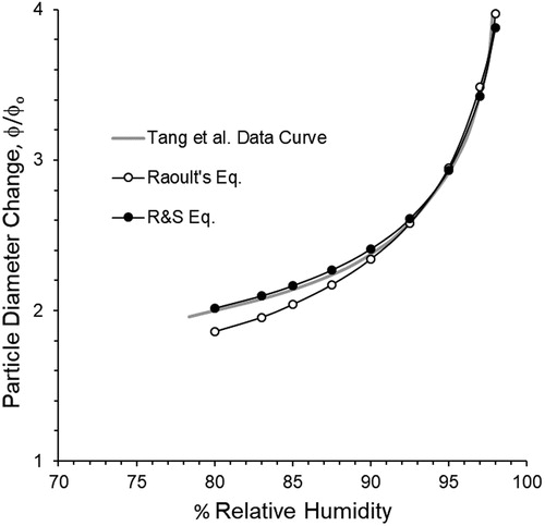
Figure 2. (a) Changes in water activity relative to mass percent of NaCl and KCl solutions. Values displayed are those reported by Robinson and Stokes (1970) and curves generated from the use of Raoult’s Law with van’t Hoff factor = 2 for both salt types. Plot (b) is the same as (a) with expansion of the water activity range near their upper limit.

In addition to the use of Raoult’s Law, $a_{\mathrm{w}}$ has also been calculated for varying droplet salt concentrations as a function of the molal osmotic coefficient, $\mathrm{\Phi },$ (Mikhailov et al. 2004; Pruppacher and Klett 2010; Robinson and Stokes 1970) (15) $$a_{\mathrm{w}}=\exp \left(-\nu \widehat{m}{M}_{\mathrm{w}}\mathrm{\Phi }/1000\right),$$(15) where $\nu$ is the number of ions a salt dissociates into (${\nu }_{\mathrm{NaCl}}=2),$ and $\widehat{m}$ is solution molality. An application of this method for the case of NaCl in water is well described by Mikhailov et al. (2004), who also demonstrate that methods to determine $\mathrm{\Phi }$ as a function of $\widehat{m}$ vary and will, therefore, affect the accuracy of the estimation of $a_{\mathrm{w}}.$

A third method for determining $a_{\mathrm{w}},$ for the case of a NaCl solution, is to apply a polynomial fit directly to measurements of $a_{\mathrm{w}}.\mathrm{ }$ A number of studies report theoretically derived and measured values of $a_{\mathrm{w}}$ relative to salt solution molality, or relative to $Y\mathrm{ }$(Chan, Kwok, and Chow 1997; Chirife and Resnik 1984; Cohen, Flagan, and Seinfeld 1987; Robinson and Stokes 1970; Tang 1996; Lehtinen et al. 2003). The NaCl $a_{\mathrm{w}}$ values published by Robinson and Stokes (R&S, 1970) are considered among the most reliable estimates and they compare closely to values published in other studies (Chan, Kwok, and Chow 1997; Chirife and Resnik 1984; Cohen, Flagan, and Seinfeld 1987; Tang 1996). We found that a cubic polynomial expression with the intercept forced to unity of the R&S $A_{\mathrm{w}}\mathrm{ }$ values regressed on $Y$ produced a nearly perfect association (r² = 1.000), and therefore was suitable for accurately representing NaCl $a_{\mathrm{w}}$ over the range of pure water to a salt solution near saturation ($\widehat{m}$ = 6 mol/kg, $Y$ = 76%) (16) $$a_{\mathrm{w}}=1-5.5741\left({10}^{-3}\right)Y-5.8805\left({10}^{-5}\right)Y^2-3.2005\left({10}^{-6}\right)Y^3.$$(16)

For comparison purposes as provided in our results, a similar expression was derived for potassium chloride (KCl) from a table of values also published by Robinson and Stokes (1970) (17) $$a_{\mathrm{w},\mathrm{KCl}}=1-4.3449\left({10}^{-3}\right)Y-2.5653\left({10}^{-5}\right)Y^2-1.3557\left({10}^{-6}\right)Y^3.$$(17)

During the core dissolution phase, the dissolving salt core is surrounded by a film of salt solution. The vapor pressure in proximity to the film surface is, therefore, interacting with the atmospheric vapor pressure to induce growth by providing a difference between $p_{\mathrm{v},\mathrm{a}}$ and $p_{\mathrm{s},\mathrm{d}}\left(T_{\mathrm{d}}\right).$ Given an available source of solid salt and rapid transfer of dissolved salt from the dissolving core to film surface, it is reasonable to assume that the film consists of a near saturated salt solution. Therefore, during the growth period when $\varphi <{1.910\varphi }_{\mathrm{p}}$ the hygroscopic model should be configured to constrain $Y.$ This point was made initially by Ferron (1977) and more recently by Longest and Hindle (2011), however, in either case, without an explanation as to implementing the constraint.

1.4. Objectives

The primary objective of this study was to determine the relationship between measured and modeled values during both the transient growth phase of a hygroscopically growing salt particle and its size at equilibrium. A secondary objective was to evaluate the effect of the method used to calculate $a_{\mathrm{w}}$ on model results. The comparison was conducted with the use of MATLAB and while incorporating either the R&S cubic expression for $a_{\mathrm{w}}$ (Equation (16)(16) $$a_{\mathrm{w}}=1-5.5741\left({10}^{-3}\right)Y-5.8805\left({10}^{-5}\right)Y^2-3.2005\left({10}^{-6}\right)Y^3.$$(16) ) or Raoult’s Law with a van’t Hoff factor of 2 to estimate $a_{\mathrm{w}}$ (Equation (14)(14) $$a_{\mathrm{w}}={\left(1+i\frac{\frac{m_{\mathrm{o}}}{M_{\mathrm{s}}}·\frac{M_{\mathrm{w}}}{{\rho }_{\mathrm{w}}}}{\frac{\pi }{6}{\varphi }^3-\frac{m_{\mathrm{o}}}{{\rho }_{\mathrm{s}}}}\right)}^{-1}={\left(1+i\frac{m_{\mathrm{w}}}{m_{\mathrm{s}}}\frac{Y/100}{1-Y/100}\right)}^{-1},$$(14) ). The comparison involved the use of previously published data and data obtained from a novel system for measuring droplet growth over time.

2. Materials and methods

2.1. Model implementation

The coupled differential equations (Equations (7)(7) $$\frac{d\varphi }{dt}=\frac{4D_{\mathrm{v}}^{\mathrm{*}}{M}_{\mathrm{w}}{p}_{\mathrm{s},\mathrm{w}}\left(T_{\mathrm{a}}\right)}{R{\rho }_{\mathrm{d}}\varphi }\left[\frac{S_{\mathrm{R}}}{T_{\mathrm{a}}}-\frac{a_{\mathrm{w}}}{T_{\mathrm{d}}}\mathrm{e}\mathrm{xp}\left[\frac{4M_{\mathrm{w}}\sigma }{R{\rho }_{\mathrm{w}}\varphi T_{\mathrm{d}}}+\frac{h_{\mathrm{fg}}{M}_{\mathrm{w}}}{R}\left(\frac{1}{T_{\mathrm{a}}}-\frac{1}{T_{\mathrm{d}}}\right)\right]\right].$$(7) and (9))(9) $$\frac{d{T}_{\mathrm{d}}}{dt}=\frac{3}{{\varphi }^2{c}_{p,\mathrm{w}}}\left[\frac{4k_{\mathrm{m}}^{\mathrm{*}}}{{\rho }_{\mathrm{d}}}\left(T_{\mathrm{a}}-T_{\mathrm{d}}\right)+h_{\mathrm{fg}}\varphi \frac{d\varphi }{dt}\right],$$(9) were solved for droplet diameter and droplet temperature, respectively, with the use of the ODE45 function in MATLAB (Ver. R2018a, MathWorks Corp., Natick, MA, USA). ODE45 calls a sub-function in which Equations (7)(7) $$\frac{d\varphi }{dt}=\frac{4D_{\mathrm{v}}^{\mathrm{*}}{M}_{\mathrm{w}}{p}_{\mathrm{s},\mathrm{w}}\left(T_{\mathrm{a}}\right)}{R{\rho }_{\mathrm{d}}\varphi }\left[\frac{S_{\mathrm{R}}}{T_{\mathrm{a}}}-\frac{a_{\mathrm{w}}}{T_{\mathrm{d}}}\mathrm{e}\mathrm{xp}\left[\frac{4M_{\mathrm{w}}\sigma }{R{\rho }_{\mathrm{w}}\varphi T_{\mathrm{d}}}+\frac{h_{\mathrm{fg}}{M}_{\mathrm{w}}}{R}\left(\frac{1}{T_{\mathrm{a}}}-\frac{1}{T_{\mathrm{d}}}\right)\right]\right].$$(7) and (9)(9) $$\frac{d{T}_{\mathrm{d}}}{dt}=\frac{3}{{\varphi }^2{c}_{p,\mathrm{w}}}\left[\frac{4k_{\mathrm{m}}^{\mathrm{*}}}{{\rho }_{\mathrm{d}}}\left(T_{\mathrm{a}}-T_{\mathrm{d}}\right)+h_{\mathrm{fg}}\varphi \frac{d\varphi }{dt}\right],$$(9) are placed along with their supporting equations, Equations (8)(8) $$D_{\mathrm{v}}^{\mathrm{*}}=D_{\mathrm{v}}{\left[\frac{1}{1+2{\delta }_{\mathrm{c}}\lambda /\varphi }+\frac{2D_{\mathrm{v}}}{\varphi {\alpha }_{\mathrm{c}}\sqrt{R{T}_{\mathrm{a}}/2\pi M_{\mathrm{w}}}}\right]}^{-1},$$(8) and (10)(10) $$k_{\mathrm{m}}^{\mathrm{*}}=k_{\mathrm{m}}{\left[\frac{1}{1+2{\delta }_{\mathrm{t}}\lambda /\varphi }+\frac{2k_{\mathrm{m}}}{\varphi {\alpha }_{\mathrm{t}}{\rho }_{\mathrm{m}}{c}_{p,\mathrm{m}}\sqrt{R{T}_{\mathrm{a}}/2\pi M_{\mathrm{a}}}}\right]}^{-1},$$(10) . Two versions were created to predict $a_{\mathrm{w}}$ with either Equation (14)(14) $$a_{\mathrm{w}}={\left(1+i\frac{\frac{m_{\mathrm{o}}}{M_{\mathrm{s}}}·\frac{M_{\mathrm{w}}}{{\rho }_{\mathrm{w}}}}{\frac{\pi }{6}{\varphi }^3-\frac{m_{\mathrm{o}}}{{\rho }_{\mathrm{s}}}}\right)}^{-1}={\left(1+i\frac{m_{\mathrm{w}}}{m_{\mathrm{s}}}\frac{Y/100}{1-Y/100}\right)}^{-1},$$(14) with a van’t Hoff factor of 2 as a function of $Y$ or Equation (16)(16) $$a_{\mathrm{w}}=1-5.5741\left({10}^{-3}\right)Y-5.8805\left({10}^{-5}\right)Y^2-3.2005\left({10}^{-6}\right)Y^3.$$(16) . Model output was written to a comma-delimited output file and imported into a spreadsheet (Excel, Microsoft Corp., Redmond, WA, USA). All discrete time steps used by ODE45 during the solution process were saved as output or user-designated time steps were selected to reduce the length of the output file. An example of the MATLAB code developed to model particle hygroscopic growth is provided in the SI. The code contains an IF statement to hold the value of $a_{\mathrm{w}}$ at its saturation value while $\varphi \le {1.910\varphi }_{\mathrm{p}}.$ This level represents a hypothetical upper limit on $Y$ within the film surrounding the dissolving salt core and therefore represents the fastest growth possible.

2.2. Model accuracy at equilibrium

For any initial particle size, the model was run over a time period until there was a <0.1% change in $\varphi$ between consecutive output timesteps (typically 0.01 s), at which time equilibrium was assumed to have been established. These values were compared to measured values of equilibrium diameter obtained from Tang, Munkelwitz, and Davis (1977) who measured equilibrium droplet diameters over a range of RH values and for a starting NaCl particle size of 400 nm. Comparisons were made after digitizing plotted points in Figure 8 of the Tang, Munkelwitz, and Davis (1977) article and determining the x–y coordinates of each data point shown relative to the scaling shown on the x and y axes of that plot.

2.3. Model accuracy during the growth phase

A novel system was developed to measure hygroscopic growth after a salt particle was instantaneously enveloped by a high humidity atmosphere. Initially, salt was aerosolized by pushing filtered, compressed air at 10 L min⁻¹ through a single-jet Collison nebulizer containing a 10% m/v salt solution. Water in the exhausted droplets evaporated as they traveled through a heated brass tube. Excess water vapor was then removed with a condenser. A glass coverslip was then passed through the exiting air stream several times to dust the coverslip with dry aerosolized salt particles.

To measure the hygroscopic growth of particles on a slide, a second system was developed to inject an atmosphere with known temperature and relative humidity onto the surface of the slide while viewing growth with the use of an inverted microscope. As shown in Figure 3, filtered, compressed air with a flow rate of 1.5 L min^–1 was directed either through a needle valve or into a glass bottle containing heated water. The air in the bottle passed through a fritter to create bubbles that maximized the transfer of water vapor into the air stream. Relative humidity was adjusted by blending the output from the bottle with air passing through the needle valve. To collect any condensed water vapor before entering the rest of the system, an impinger was placed in-line as a water trap. The combined flow was directed through a 4-way tube fitting. Relative humidity and temperature were measured with a sensor (Model HM70, Vaisala, Helsinki, Finland) every 0.5 s for the duration of the experiment. The probe of the sensor was wrapped with Teflon® tape to create a tight seal and extended down through the upper hole of the fitting and into the center area. The probe was previously calibrated using a two-point calibration procedure in which the probe was tightly sealed in a container containing a saturated KNO₃ solution and then a saturated NaCl solution, which produces equilibrium RH levels of 75.41% and 94.53%, respectively.

Figure 3. Schematic diagram of the hygroscopic growth and video-capture system.

Exhaust air traveled through one of two solenoid valves controlled by a software routine created in LabVIEW (National Instruments, Austin, TX, USA). The routine was also coded to continuously monitor the RH level measured with the sensor (temperature was noted at intervals by the operator). The solenoid valves were operated simultaneously so that only one was open at any time. During startup, the open solenoid valve allowed air through the system to exhaust into the atmosphere of the laboratory until the desired RH was consistently measured. The on/off pattern of the solenoids was then switched to direct the high relative humidity air onto the microscope slide via a short tube connected to a custom-made glass tube with a downward curving exit hole. The glass tube exit hole was first pointed away from the slide to fill the tube with the humidified air. The entire switching process was then repeated after pointing the exit hole onto the slide containing the particles.

The slide was placed on an inverted microscope (CKX31, Olympus Corp., Center Valley, PA, USA) set to ×400 magnification. A cell phone (SM-G965U1, Samsung Corp., Seoul, South Korea) was mounted via an eyepiece attachment so that its camera could video record particles on a slide. The digital magnification of the cell phone was maximized and the slide was positioned to have a single particle in the video stream at the best clarity. Particle growth was recorded for at least 30 s. After a trial, a video recording was also briefly made of a stage micrometer with scaling every 0.1 mm. Both video recordings were then processed by a video-to-JPG conversion software (DVDVideoSoft, Digital Wave Ltd.) to extract and save individual frames of the video. The cell phone was set to video record at the standard capture rate of 30 photos s⁻¹ or once every 0.033 s. Micrograph analysis software (Image J) was used to measure the diameter of a particle in photos spanning a 30 s trial. Only the diameters in successive micrographs that revealed a noticeable increase from a previously measured micrograph were recorded in a spreadsheet. The image resolution was 0.1 µm pixel^–1. Of the particles available to be viewed in a micrograph, one with a clear outline and distant from other particles was measured. The spreadsheet was also used to convert pixel distance to actual distance from their ratio obtained from the extracted micrograph of the stage micrometer. The start of the growth process was the micrograph just before the first frame that revealed any change in the shape or coloration of the measured particle.

An example of micrographs of a growing droplet is given in SI Figure S.1. From a geometric viewpoint, the particle diameter measurements were those of the base of a hemispherical cap. The volume of that cap depends on its contact angle, which is approximately 40° for a salt solution droplet on a glass plate (Sghaier, Prat, and Nasrallah 2006). Here we assumed the quickly growing droplet starting from a dry particle would assume a hemispherical shape (contact angle = 90°) to simplify calculations and given that relative comparison between the diameter of this droplet on glass and the modeled diameter of a spherical droplet explained below. With that assumption, the volume of the hemisphere was calculated, and a volume equivalent diameter (${\mathrm{\Phi }}_{\mathrm{EV}},$ diameter of a sphere with equal volume) was computed from each measurement by dividing that measurement by the cube root of 2.

At least six trials were conducted by two of the authors independently to ensure the repeatability of the measurement process. Three trials were chosen from each set based on the criteria that the RH during a trial remained within ±0.3% of the average RH value over the 30-s trial. The six trials were conducted at temperatures between 23 and 25 °C and RH between 98% and 100%. As shown in Figure 4 of the Li, Montassier, and Hopke (1992) article, air temperature differences between 22 and 37 °C have a negligible effect on particle growth. Therefore, these trials conducted at room temperatures are relevant to lung temperatures approaching 37 °C.

Figure 4. Modeled growth curve (a) of a 1000 nm NaCl particle in 37 °C (310.15 K), 99.5% RH atmosphere, and modeled droplet temperature (b). The inset for plot (a) expands the time scale of the larger plot; the open circle indicates the point on the curve related to the time at which the particle has fully dissolved before which its solution concentration was constrained to its saturation value.

Trial results were then compared to results from the growth model implemented in MATLAB given the trial average RH and temperature, and ${\mathrm{\Phi }}_{\mathrm{EV}}$ of the dry particle measured. Given that the three-dimensional structure of the dry particle was not measurable, and therefore the initial mass of salt was unknown, the starting mass of the salt was adjusted until the root mean squared error (RMSE) of measured-to-modeled results over the 30-s trial period were minimized. This adjustment, therefore, resulted in a comparison of the growth patterns developed by the measured droplet on the coverslip to that of the modeled values for the same RH and temperature over the entire growth curve, but, in particular, a comparison of the relationship between measured–modeled pairs during the initial fast-growth period.

3. Results and discussion

3.1. Model output

Figure 4 displays model results of the typical pattern of droplet growth over time in a high humidity environment (RH = 99.5%) for a 1000 nm NaCl particle. Plot (a) of Figure 4 shows very rapid initial growth followed by a slower growth period as the droplet size transitions to its equilibrium size. The inset for plot (a) expands the time scale during the first 0.02 s that coincided with the time during which $\varphi <{1.910\varphi }_{\mathrm{p}}$ and $a_{\mathrm{w}}$ was fixed at its saturation value. Although essentially linear over this short time period, growth during this time follows a steeply upward curving trajectory of growth established by maximizing $d\varphi /dt$ (Equation (7)(7) $$\frac{d\varphi }{dt}=\frac{4D_{\mathrm{v}}^{\mathrm{*}}{M}_{\mathrm{w}}{p}_{\mathrm{s},\mathrm{w}}\left(T_{\mathrm{a}}\right)}{R{\rho }_{\mathrm{d}}\varphi }\left[\frac{S_{\mathrm{R}}}{T_{\mathrm{a}}}-\frac{a_{\mathrm{w}}}{T_{\mathrm{d}}}\mathrm{e}\mathrm{xp}\left[\frac{4M_{\mathrm{w}}\sigma }{R{\rho }_{\mathrm{w}}\varphi T_{\mathrm{d}}}+\frac{h_{\mathrm{fg}}{M}_{\mathrm{w}}}{R}\left(\frac{1}{T_{\mathrm{a}}}-\frac{1}{T_{\mathrm{d}}}\right)\right]\right].$$(7) ) when maintaining $a_{\mathrm{w}}$ at its minimum value. Droplet temperature during the initial 0.1 s of growth is shown in Figure 4b. As can be seen in that plot, the temperature output fluctuates rapidly by approximately ±0.3 °C at any time point as a consequence of the solutions obtained by ODE45 during successive micro-second time steps. Furthermore, plot (b) reveals that droplet temperature remained stable for approximately 0.016 s, which also coincides with the time when $\varphi <{1.910\varphi }_{\mathrm{p}}$ after which the IF statement released the constraint on the droplet solution concentration at saturation. That plot also suggests that the addition of Equation (9)(9) $$\frac{d{T}_{\mathrm{d}}}{dt}=\frac{3}{{\varphi }^2{c}_{p,\mathrm{w}}}\left[\frac{4k_{\mathrm{m}}^{\mathrm{*}}}{{\rho }_{\mathrm{d}}}\left(T_{\mathrm{a}}-T_{\mathrm{d}}\right)+h_{\mathrm{fg}}\varphi \frac{d\varphi }{dt}\right],$$(9) in the model only has an effect during the rapid initial-growth phase of droplet growth after which droplet temperature quickly approaches ambient temperature.

Figure 5 provides another demonstration of model output with regards to differences in salt properties and the estimation of${\mathrm{ }a}_{\mathrm{w}}.$ Models of KCl water activity were developed in a manner similar to those developed for NaCl (Equation (14)(14) $$a_{\mathrm{w}}={\left(1+i\frac{\frac{m_{\mathrm{o}}}{M_{\mathrm{s}}}·\frac{M_{\mathrm{w}}}{{\rho }_{\mathrm{w}}}}{\frac{\pi }{6}{\varphi }^3-\frac{m_{\mathrm{o}}}{{\rho }_{\mathrm{s}}}}\right)}^{-1}={\left(1+i\frac{m_{\mathrm{w}}}{m_{\mathrm{s}}}\frac{Y/100}{1-Y/100}\right)}^{-1},$$(14) with $i$ = 2 and Equation (17)(17) $$a_{\mathrm{w},\mathrm{KCl}}=1-4.3449\left({10}^{-3}\right)Y-2.5653\left({10}^{-5}\right)Y^2-1.3557\left({10}^{-6}\right)Y^3.$$(17) ). First, referring to Figure 2, it can be seen that KCl has higher $a_{\mathrm{w}}$ values than NaCl for any $Y\mathrm{ }$ which causes a higher estimate of droplet surface vapor pressure ${(p}_{\mathrm{s},\mathrm{d}})$ and therefore a lower computed vapor pressure differential between ambient, $p_{\mathrm{v},\mathrm{a}},$ and droplet surface, $p_{\mathrm{s},\mathrm{d}},$ vapor pressures (Equation (3)(3) $$\frac{d\varphi }{dt}=\frac{4D_{\mathrm{v}}^{\mathrm{*}}{M}_{\mathrm{w}}}{R{\rho }_{\mathrm{d}}\varphi }\left[\frac{p_{\mathrm{v},\mathrm{a}}}{T_{\mathrm{a}}}-\frac{p_{\mathrm{s},\mathrm{d}}\left(T_{\mathrm{d}}\right)}{T_{\mathrm{d}}}\right],$$(3) ) that results in less hygroscopic growth before reaching equilibrium. The consequence of this difference is shown in Figure 5a, where KCl growth is noticeably less than that of NaCl. Figure 5a also demonstrates that the equilibrium diameter, and therefore the reported “growth factor” depends on the estimation of${\mathrm{ }a}_{\mathrm{w}}.$ For both salts, the use of Raoult’s Law produces a larger equilibrium diameter than the R&S equation when modeling at high humidity (99.5% RH). As shown in Figure 2b, for the same $Y,$ Raoult’s Law predicts a lower $a_{\mathrm{w}}$ value than the R&S equation as $Y$ reaches its minimum, and therefore $a_{\mathrm{w}}$ is high. A lower $a_{\mathrm{w}}$ value represents a lower vapor pressure exerted at the droplet surface and, therefore, a greater difference between $p_{\mathrm{v},\mathrm{a}}$ and $p_{\mathrm{s},\mathrm{d}},$ which results in more growth as it approaches equilibrium. This effect is more pronounced for KCl than for NaCl because Raoult’s Law for KCl is greater than the R&S equation for KCl over a wider range of$\mathrm{ }Y.$ An effect related to the choice of the equation to estimate a_w is also shown in Figure 5a. Here, the use of Raoult’s Law to model KCl produces a growth curve almost identical to NaCl modeled with the use of the R&S values.

Figure 5. Modeled KCl and NaCl growth curves using either Raoult’s equation or Equation (19) based on Robinson and Stokes values (R&S) to calculate water activity. Modeling was performed with a temperature of 37 °C and 99.5% RH. (a) Comparison of entire growth curves developed for both salt types and both water activity equations. (b) Initial growth period when modeling NaCl using both equations and when no constraint is applied to the saturation of the growing droplet.

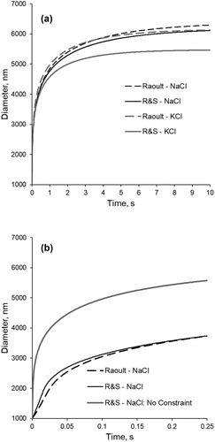
Figure 5b shows the opposite effect during the initial growth period – the R&S equation produces faster growth than Raoult’s equation – because the R&S equation predicts lower $a_{\mathrm{w}}$ values than does Raoult’s Law for the same $Y.$ For comparison, the initial growth curve is produced when no constraint is placed on the droplet surface concentration during the initial growth phase is also shown in Figure 5b, resulting in rapid growth relative to growth when the constraint is applied.

3.2. Model accuracy at equilibrium

Modeled diameter change (growth ratio), $\varphi /{\varphi }_0,$ using the R&S equation closely compares to a best-fit curve established by Tang, Munkelwitz, and Davis (1977) throughout the range of RH over which they obtained measured values (see Figure 6). Whereas, modeled values using Raoult’s Law underestimate $\varphi /{\varphi }_0$ at low RH and overestimate $\varphi /{\varphi }_0$ at high RH (>95%). This comparison demonstrates that the relationship between Raoult’s equation and the R&S equation for $a_{\mathrm{w}}$ discussed in the preceding section is only valid for high RH conditions. As shown in Figure 6, Raoult’s Law underpredicts $\varphi /{\varphi }_0$ to an increasingly greater extent as RH approaches ${\mathrm{RH}}_{\mathrm{o}}.$ This result can also be explained by the relationship in model output resulting from the use of the two equations shown in Figure 2. In this case, Figure 2a reveals the Raoult’s Law predicts higher $a_{\mathrm{w}}$ values relative to $Y\mathrm{ }$ when $a_{\mathrm{w}}$ values are low, which are the case for equilibrium at low RH. These higher $a_{\mathrm{w}}$ values result in the lower predicted growth ratios shown in Figure 6.

Figure 6. Comparison of modeled values to measurements made by Tang et al. during deliquescence experiments using 400 nm NaCl particles at 25 °C and the RH noted on the x-axis.

3.3. Model accuracy during the initial growth phase

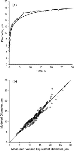
A comparison of ${\varphi }_{\mathrm{EV}}$ obtained with the use of the video capture method with droplet diameters obtained from the hygroscopic growth model while using the R&S model (Equation (16)(16) $$a_{\mathrm{w}}=1-5.5741\left({10}^{-3}\right)Y-5.8805\left({10}^{-5}\right)Y^2-3.2005\left({10}^{-6}\right)Y^3.$$(16) ) to calculate water activity for one representative trial is given in Figure 7a. The measured trial environmental conditions were 26 °C and 98.9% RH. Figure 7a demonstrates relatively close agreement between the trend of growth developed by the model with measurements over the extent of the 30-s trial. A comparison of coincidental values (measured and modeled at the same time point) for data from all six trials is shown in Figure 7b. As shown, the points are highly correlated (r = 0.975) and are clustered near the 1:1 line. Some points associated with the largest droplet sizes deviate from the 1:1 relationship, which are primarily associated with one of the six trials that did not produce a measured growth curve that followed the trend of the modeled curve as the droplets approached equilibrium.

Figure 7. Comparison of modeled and measured values when using the Robinson and Stokes equation to compute water activity. (a) Example of comparison between measured values and model curve – results from one trial. (b) Correlation of all measured-to-modeled pairs for the six trials – dashed line indicates a 1:1 relationship.

The results provided in Figure 7b suggest that the initial growth curve developed with the use of Equation (16)(16) $$a_{\mathrm{w}}=1-5.5741\left({10}^{-3}\right)Y-5.8805\left({10}^{-5}\right)Y^2-3.2005\left({10}^{-6}\right)Y^3.$$(16) to predict $a_{\mathrm{w}}$ and with a constraint on its saturation value during the deliquescence growth phase is valid when modeling NaCl hygroscopic growth. Table 1 provides results from a linear regression analysis comparing measured to modeled values for the three water activity model options evaluated in this study for all points collected over 30 s and for points obtained during the initial growth phase when $\varphi <{1.910\varphi }_{\mathrm{p}}.$ Over the entire growth period and during the initial growth phase, the use of the R&S values to produce Equation (16)(16) $$a_{\mathrm{w}}=1-5.5741\left({10}^{-3}\right)Y-5.8805\left({10}^{-5}\right)Y^2-3.2005\left({10}^{-6}\right)Y^3.$$(16) and constrained to the saturation level of NaCl while $\varphi <{1.910\varphi }_{\mathrm{p}}$ produced the best fit to the measured values (lowest RMSE and highest R²).

Table 1. Summary of comparisons between modeled and measured results for three variations of the water activity calculation in the hygroscopic growth model.

	RMSE	Slope	Intercept	R^2
Measurements over 30 s
R&S constrained	1.007	0.979	0.008	0.950
Raoult’s law constrained	1.392	0.977	−0.374	0.923
R&S unconstrained	1.649	0.740	3.602	0.887
Measurements when φ < 1.905φp
R&S constrained	0.607	0.930	0.596	0.892
Raoult’s law constrained	0.865	0.816	1.000	0.814
R&S unconstrained	2.247	1.061	1.438	0.718

Admittedly, the use of Raoult’s law to calculate $a_{\mathrm{w}}$ (Equation (14)(14) $$a_{\mathrm{w}}={\left(1+i\frac{\frac{m_{\mathrm{o}}}{M_{\mathrm{s}}}·\frac{M_{\mathrm{w}}}{{\rho }_{\mathrm{w}}}}{\frac{\pi }{6}{\varphi }^3-\frac{m_{\mathrm{o}}}{{\rho }_{\mathrm{s}}}}\right)}^{-1}={\left(1+i\frac{m_{\mathrm{w}}}{m_{\mathrm{s}}}\frac{Y/100}{1-Y/100}\right)}^{-1},$$(14) ) produced almost identical regression results as when using the R&S equation across the entire growth period. However, the differences between the two methods are more significant during the initial growth phase. As expected, Raoult’s law underestimates the measured values during this time (slope = 0.816) relative to when using the R&S equation (slope = 0.930) for reasons explained earlier. To best demonstrate the consequences of using Raoult’s law to approximate $a_{\mathrm{w}}$ we purposely simplified the growing droplet solution to that of a binary mixture containing a salt with well-established properties from which the relationship between $a_{\mathrm{w}}$ and $Y$ could be nearly exactly parameterized with the use of a polynomial expression (Equation (16)(16) $$a_{\mathrm{w}}=1-5.5741\left({10}^{-3}\right)Y-5.8805\left({10}^{-5}\right)Y^2-3.2005\left({10}^{-6}\right)Y^3.$$(16) ). The dependence on the use of some form of Raoult’s law results from the need to minimize computationally expensive algorithms applied to CFD models of particle deposition in the lung, especially those involving multi-component pharmaceuticals (Chen et al. 2017; Longest and Hindle 2011). However, advances on this issue in the field of atmospheric sciences may serve to enhance the accuracy of $a_{\mathrm{w}}$ models without sacrificing computation time (Petters and Kreidenweis 2007; Nenes, Pandis, and Pilinis 1998; Zuend et al. 2008).

The application of a constraint on $Y$ applied to the R&S equation while $\varphi <{1.910\varphi }_{\mathrm{p}}$ produced much better associations between measured and modeled results than when left unconstrained. Use of the unconstrained R&S equation produced a low slope relative to unity and high intercept (Table 1) resulting from the overestimation of droplet size during the initial growth phase under this condition. Furthermore, a slope of 0.979 obtained when the constrained R&S equation was applied suggests that the assumption that the film layer around the dissolving core is at saturation is valid for modeling NaCl. A consequence of this constraint on the growth profile was to produce a rapid increase in droplet diameter while the constraint was imposed. However, when comparing measurements with modeled results during the time period when $\varphi <{1.910\varphi }_{\mathrm{p}},$ the slopes resulting when the R&S constraint was imposed (0.930) relative to when it was not imposed (1.061) are nearly identical. This suggests that the constraint may be relaxed to a more realistic level near, but not equal to, saturation.

The assumption that the film layer remains near saturation while $\varphi <{1.910\varphi }_{\mathrm{p}}$ may not be true for other salts as it will only occur when the rate of dissolution of the salt core is high relative to the water uptake rate of the growing droplet. Increasing the accuracy of the hygroscopic model by incorporating the kinetics associated with the dissolving salt core is a research topic of interest (Bahadur and Russell 2008; Asa-Awuku and Nenes 2007; Lehtinen et al. 2003). However, for NaCl, these results suggest that the relatively simple assumption that the salt core readily dissolves, and that the salt ions immediately mix throughout the film layer to consistently form a saturated solution while the core dissolves, is valid.

Furthermore, the equations given by Broday and Georgopoulos (2001) followed here to model hygroscopic growth do not consider the thermodynamics associated with a dissolving salt core. Salt dissolution absorbs heat that is otherwise released during condensation (Tang and Munkelwitz 1992), which affects the water activity value for a given temperature and therefore affects ${\mathrm{RH}}_0$ (Chen 1994). However, Van Campen, Amidon, and Zografi (1983) state that this heat of dissolution is negligible for most alkali halide salts compared with the heat of condensation and, therefore, its inclusion in Equation (9)(9) $$\frac{d{T}_{\mathrm{d}}}{dt}=\frac{3}{{\varphi }^2{c}_{p,\mathrm{w}}}\left[\frac{4k_{\mathrm{m}}^{\mathrm{*}}}{{\rho }_{\mathrm{d}}}\left(T_{\mathrm{a}}-T_{\mathrm{d}}\right)+h_{\mathrm{fg}}\varphi \frac{d\varphi }{dt}\right],$$(9) may not provide additional accuracy when modeling NaCl, but could be important when modeling other hygroscopic particle types.

The results presented here are particularly important when using the hygroscopic growth model to determine the growth of particles entering the lungs. Given the fast transit time of a particle from mouth to lung bifurcations, the accuracy of the growth model during the initial growth phase is critical for accurately estimating the eventual deposition of the particle. For particles with hygroscopic properties similar to NaCl, model results indicate that particles larger than 140 nm entirely within a 99.5% RH environment will not reach equilibrium within the 0.2 s transit time to the first bifurcation (Longest and Hindle 2011). Furthermore, particle sizes considered optimal for delivery of inhaled pharmaceuticals are in the micrometer size range (Lee et al. 2009; Zanen, Go, and Lammers 1996) and therefore likely to be still in the initial growth phase when deposited. The gradient in ambient RH between that of the atmosphere and its condition within the deep lung will also increase the length of the initial growth phase (Ferron, Kreyling, and Haider 1988). The results provided by Anselm et al. (1986) and Martonen et al. (1982), in addition to growth reactor results we provide in the SI (Figures S.2 and S.3), demonstrate much slower growth as a particle enters the lung that would require an additional sophistication of the model to include temperature and relative humidity changes over time as well as turbulent mixing only capable when incorporating the hygroscopic growth model within a CFD model of the lung such as described by Longest and Hindle (2011). Our future work will involve further validation of the hygroscopic growth model within human lung conditions.

4. Conclusions

The hygroscopic growth model, as formulated by Broday and Georgopoulos (2001), is valid throughout the entire hygroscopic growth of single NaCl solution droplet. Model validity is enhanced when applying an estimation of water activity that is accurate throughout the entire range of droplet salt solution concentrations encountered during hygroscopic growth from a dry salt particle to a droplet at equilibrium with ambient water vapor pressure. In that regard, we found that a cubic expression developed from values published by Robinson and Stokes (1970) to calculate water activity resulted in modeled results that compared well with measured values both at equilibrium diameters and during the initial growth phase. Model accuracy during the initial growth phase is particularly essential for particles entering the humid environment of the lung that are too large to reach equilibrium before entering the lower branches of the pulmonary system, which will therefore improve the accuracy of deposition site estimation within the lung.

Additional information

Funding

This work was supported by the FDA under Grant U01-FD005837; the NIEHS under Grant P30 ES005605; CDC/NIOSH under Grant T42OH008491; and the NIH (Center for Scientific Review) under Grant U01-HL114494.

References

- Anselm, A., J. Gebhart, J. Heyder, and G. Ferron. 1986. Human inhalation studies of growth of hygroscopic particles in the respiratory tract. Paper presented at the Aerosols: Formation and Reactivity. Proceedings of the 2nd International Aerosol Conference, Berlin, Germany, 252–5.
- Asa-Awuku, A., and A. Nenes. 2007. Effect of solute dissolution kinetics on cloud droplet formation: Extended Köhler theory. J. Geophys. Res. Atmos. 112 (D2201): 1–10. doi:10.1029/2005JD006934.
- Asgharian, B. 2004. A model of deposition of hygroscopic particles in the human lung. Aerosol Sci. Technol. 38 (9):938–47. doi:10.1080/027868290511236.
- Bahadur, R., and L. M. Russell. 2008. Water uptake coefficients and deliquescence of NaCl nanoparticles at atmospheric relative humidities from molecular dynamics simulations. J. Chem. Phys. 129 (9):094508. doi:10.1063/1.2971040.
- Bates, D. V., B. R. Fish, T. F. Hatch, T. T. Mercer, and P. Morrow. 1966. Deposition and retention models for internal dosimetry fo the human respiratory tract: Task Group on Lung Dynamics. Health Phys. 12:173–207.
- Broday, D. M., and P. G. Georgopoulos. 2001. Growth and deposition of hygroscopic particulate matter in the human lungs. Aerosol Sci. Technol. 34 (1):144–59. doi:10.1080/02786820118725.
- Chan, C. K., C. S. Kwok, and A. H. L. Chow. 1997. Study of hygroscopic properties of aqueous mixtures of disodium fluorescein and sodium chloride using an electrodynamic balance. Pharm. Res. 14 (9):1171–5. doi:10.1023/A:1012146621821.
- Chen, J.-P. 1994. Theory of deliquescense and modified Köhler curves. J. Atmos. Sci. 51 (23):3505–16. doi:10.1175/1520-0469(1994)051<3505:TODAMK>2.0.CO;2.
- Chen, X., Y. Feng, W. Zhong, and C. Kleinstreuer. 2017. Numerical investigation of the interaction, transport and deposition of multicomponent droplets in a simple mouth–throat model. J. Aerosol Sci. 105:108–27. doi:10.1016/j.jaerosci.2016.12.001.
- Chirife, J., and S. L. Resnik. 1984. Unsaturated solutions of sodium chloride as reference sources of water activity at various temperatures. J. Food Sci. 49 (6):1486–8. doi:10.1111/j.1365-2621.1984.tb12827.x.
- Cohen, M. D., R. C. Flagan, and J. H. Seinfeld. 1987. Studies of concentrated electrolyte solutions using the electrodynamic balance. I. Water activities for single-electrolyte solutions. J. Phys. Chem. 91 (17):4563–74. doi:10.1021/j100301a029.
- Cruz, C. N., and S. N. Pandis. 2000. Deliquescence and hygroscopic growth of mixed inorganic–organic atmospheric aerosol. Environ. Sci. Technol. 34 (20):4313–19. doi:10.1021/es9907109.
- Djikaev, Y. S., R. Bowles, H. Reiss, K. Hämeri, A. Laaksonen, and M. Väkevä. 2001. Theory of size dependent deliquescence of nanoparticles: Relation to heterogeneous nucleation and comparison with experiments. J. Phys. Chem. B 105 (32):7708–22. doi:10.1021/jp010537e.
- Ewing, G. E. 2005. H2O on NaCl: From single molecule, to clusters, to monolayer, to thin film, to deliquescence. In Intermolecular forces and clusters II, Structure and bonding, ed. D. J. Wales, vol. 116, 1–25. New York: Springer.
- Feng, Y., C. Kleinstreuer, N. Castro, and A. Rostami. 2016. Computational transport, phase change and deposition analysis of inhaled multicomponent droplet–vapor mixtures in an idealized human upper lung model. J. Aerosol Sci. 96:96–123. doi:10.1016/j.jaerosci.2016.03.001.
- Ferron, G. A. 1977. The size of soluble aerosol particles as a function of the humidity of the air. Application to the human respiratory tract. J. Aerosol Sci. 8 (4):251–67. doi:10.1016/0021-8502(77)90045-3.
- Ferron, G. A., W. G. Kreyling, and B. Haider. 1988. Inhalation of salt aerosol particles. II. Growth and deposition in the human respiratory tract. J. Aerosol Sci. 19 (5):611–31. doi:10.1016/0021-8502(88)90213-3.
- Finlay, W. H. 2001. The mechanics of inhaled pharmaceutical aerosols: An introduction. Cambridge, MA: Academic Press.
- Fredenslund, A., J. Gmehling, M. L. Michelsen, P. Rasmussen, and J. M. Prausnitz. 1977. Computerized design of multicomponent distillation columns using the UNIFAC group contribution method for calculation of activity coefficients. Ind. Eng. Chem. Proc. Des. Dev. 16 (4):450–62. doi:10.1021/i260064a004.
- Hemminger, J. C. 1999. Heterogeneous chemistry in the troposphere: A modern surface chemistry approach to the study of fundamental processes. Int. Rev. Phys. Chem. 18 (3):387–417. doi:10.1080/014423599229929.
- Hinds, W. C. 1999. Aerosol technology: Properties, behavior, and measurement of airborne particles. Vol. 2. New York: Wiley.
- Lee, S. L., W. P. Adams, B. V. Li, D. P. Conner, B. A. Chowdhury, and X. Y. Lawrence. 2009. In vitro considerations to support bioequivalence of locally acting drugs in dry powder inhalers for lung diseases. AAPS J. 11 (3):414–23. doi:10.1208/s12248-009-9121-4.
- Lehtinen, K. E. J., M. Kulmala, P. Ctyroky, T. Futschek, and R. Hitzenberger. 2003. Effect of electrolyte diffusion on the growth of NaCl particles by water vapour condensation. J. Phys. Chem. A 107 (3):346–50. doi:10.1021/jp020240w.
- Li, W., N. Montassier, and P. K. Hopke. 1992. A system to measure the hygroscopicity of aerosol particles. Aerosol Sci. Technol. 17 (1):25–35. doi:10.1080/02786829208959557.
- Longest, P. W., and M. Hindle. 2011. Numerical model to characterize the size increase of combination drug and hygroscopic excipient nanoparticle aerosols. Aerosol Sci. Technol. 45 (7):884–99. doi:10.1080/02786826.2011.566592.
- Longest, P. W., J. T. McLeskey, Jr., and M. Hindle. 2010. Characterization of nanoaerosol size change during enhanced condensational growth. Aerosol Sci. Technol. 44 (6):473–83. doi:10.1080/02786821003749525.
- Low, R. D. H. 1969. A generalized equation for the solution effect in droplet growth. J. Atmos. Sci. 26 (3):608–11. doi:10.1175/1520-0469(1969)026<0608:AGEFTS>2.0.CO;2.
- Marcolli, C., and U. K. Krieger. 2006. Phase changes during hygroscopic cycles of mixed organic/inorganic model systems of tropospheric aerosols. J. Phys. Chem. A 110 (5):1881–93. doi:10.1021/jp0556759.
- Martin, S. T. 2000. Phase transitions of aqueous atmospheric particles. Chem. Rev. 100 (9):3403–54. doi:10.1021/cr990034t.
- Martonen, T. B., K. A. Bell, R. F. Phalen, A. F. Wilson, and A. Ho. 1982. Growth rate measurements and deposition modelling of hygroscopic aerosols in human tracheobronchial models. In Inhaled particles V, ed. W. H. Walton, 93–108. New York: Elsevier.
- Mauer, L. J., and L. S. Taylor. 2010. Water-solids interactions: Deliquescence. Annu. Rev. Food Sci. Technol. 1 (1):41–63. doi:10.1146/annurev.food.080708.100915.
- Mikhailov, E., S. Vlasenko, R. Niessner, and U. Pöschl. 2004. Interaction of aerosol particles composed of protein and saltswith water vapor: Hygroscopic growth and microstructural rearrangement. Atmos. Chem. Phys. 4 (2):323–50. doi:10.5194/acp-4-323-2004.
- Ming, Y., and L. M. Russell. 2001. Predicted hygroscopic growth of sea salt aerosol. J. Geophys. Res. 106 (D22):28259–74. doi:10.1029/2001JD000454.
- Moore, R. H., and T. M. Raymond. 2008. HTDMA analysis of multicomponent dicarboxylic acid aerosols with comparison to UNIFAC and ZSR. J. Geophys. Res. 113 (D4):1–15. doi:10.1029/2007JD008660.
- Nenes, A., S. N. Pandis, and C. Pilinis. 1998. ISORROPIA: A new thermodynamic equilibrium model for multiphase multicomponent inorganic aerosols. Aquatic Geochem. 4 (1):123–52. doi:10.1023/A:1009604003981.
- Petters, M. D., and S. M. Kreidenweis. 2007. A single parameter representation of hygroscopic growth and cloud condensation nucleus activity. Atmos. Chem. Phys. (European Geosciences Union) 7 (8):1961–1971.
- Pruppacher, H. R., and J. D. Klett. 2010. Microphysics of clouds and precipitation. In Atmospheric and oceanographic sciences library, ed. L. A. Mysak and K. Hamilton. Vol. 18, 2nd ed, 107–111, 502–511 New York: Springer.
- Rader, D. J., and P. H. McMurry. 1986. Application of the tandem differential mobility analyzer to studies of droplet growth or evaporation. J. Aerosol Sci. 17 (5):771–87. doi:10.1016/0021-8502(86)90031-5.
- Robinson, R. A., and R. H. Stokes. 1970. Electrolyte solutions: The measurement and interpretation of conductance, chemical potential and diffusion in solutions of simple electrolytes. 2nd ed. London: Butterworths.
- Robinson, R. J., and C. P. Yu. 1998. Theoretical analysis of hygroscopic growth rate of mainstream and sidestream cigarette smoke particles in the human respiratory tract. Aerosol Sci. Technol. 28 (1):21–32. doi:10.1080/02786829808965509.
- Russell, L. M., and Y. Ming. 2002. Deliquescence of small particles. J. Chem. Phys. 116 (1):311–21. doi:10.1063/1.1420727.
- Seinfeld, J. H., and S. N. Pandis. 2016. Atmospheric chemistry and physics: From air pollution to climate change. New York: Wiley.
- Sghaier, N., M. Prat, and S. B. Nasrallah. 2006. On the influence of sodium chloride concentration on equilibrium contact angle. Chem. Eng. J. 122 (1–2):47–53. doi:10.1016/j.cej.2006.02.017.
- Tang, I. N. 1996. Chemical and size effects of hygroscopic aerosols on light scattering coefficients. J. Geophys. Res. 101 (D14):19245–50. doi:10.1029/96JD03003.
- Tang, I. N., and H. R. Munkelwitz. 1993. Composition, temperature dependence of the deliquescence properties of hygroscopic aerosols. Atmos. Environ. Part A Gen Top. 27 (4):467–73.
- Tang, I. N., H. R. Munkelwitz, and J. G. Davis. 1977. Aerosol growth studies. II. Preparation and growth measurements of monodisperse salt aerosols. J. Aerosol Sci. 8 (3):149–59. doi:10.1016/0021-8502(77)90002-7.
- Van Campen, L. G. L. Amidon, and G. Zografi. 1983. Moisture sorption kinetics for water-soluble substances. I. Theoretical considerations of heat transport control. J. Pharm. Sci. 72 (12):1381–8. doi:10.1002/jps.2600721204.
- Winkler-Heil, R., G. Ferron, and W. Hofmann. 2014. Calculation of hygroscopic particle deposition in the human lung. Inhal. Toxicol. 26 (3):193–206. doi:10.3109/08958378.2013.876468.
- Zanen, P., L. T. Go, and J. W. Lammers. 1996. Optimal particle size for beta 2 agonist and anticholinergic aerosols in patients with severe airflow obstruction. Thorax 51 (10):977–80. doi:10.1136/thx.51.10.977.
- Zuend, A., C. Marcolli, B. P. Luo, and T. Peter. 2008. A thermodynamic model of mixed organic-inorganic aerosols to predict activity coefficients. Atmos. Chem. Phys. Discuss. 8 (2):6069–151. doi:10.5194/acpd-8-6069-2008.