Closure between particulate matter concentrations measured ex situ by thermal–optical analysis and in situ by the CPMA–electrometer reference mass system

Abstract

The thermal-optical analysis (TOA) of black carbon in particulate matter (PM) collected on filters has been recommended and used for the calibration of mass-concentration instruments. However, filter-based TOA calibrations have substantial practical limitations, requiring high sample flow rates (>10 litres per minute), long sampling times (up to 3 h), and subsequently manual filter processing with long analysis times (>15 min per filter). These limitations are avoided by in situ calibration techniques such as the centrifugal particle mass analyzer (CPMA)–electrometer reference mass system (CERMS). The CERMS is capable of producing and monitoring in situ reference mass concentrations below 1 µg m⁻³ and in real-time (∼1 Hz). Additional advantages of the CERMS are its improved repeatability (1.1%) over TOA (9–11%), and its measurement of a well-defined quantity: total post-CPMA suspended PM mass. In the present work, we demonstrate closure between these two techniques in terms of PM mass concentration for three different soot generators (viz., the Argonaut miniature inverted soot generator, Jing miniCAST, and National Research Council inverted-flame burner) under carefully controlled conditions. We also demonstrate the sensitivity of the CERMS by characterizing the limits of detection of a commercial laser-induced incandescence instrument and a photoacoustic instrument. Our data support the use of the CERMS with well-characterized PM sources to provide reference mass concentrations for the calibration of instruments measuring PM or black-carbon mass concentration.

EDITOR:

• Jingkun Jiang

1. Introduction

Black carbon (BC) is an important component of the radiative balance of the Earth (Bond et al. 2013) and has been implicated in the negative cardiovascular health impacts of air pollution (Grahame, Klemm, and Schlesinger 2014; Oberdörster, Oberdörster, and Oberdörster 2005; Purser, Maynard, and Wakefield 2015). The most common form of BC is soot BC (Corbin et al. 2019): the light-absorbing, insoluble, refractory aggregates of highly graphitized nanoparticles abundantly produced from the gas phase during the combustion of hydrocarbons (Bond and Bergstrom 2006; Bond et al. 2013; Petzold et al. 2013). This soot BC is routinely measured by several different techniques based on its light absorption, vaporization temperature, or other properties (Petzold et al. 2013).

A common technique for quantifying soot BC is thermal–optical analysis (TOA) (Cavalli et al. 2010; Chow et al. 2007; Watson, Chow, and Chen 2005). Based on the method introduced by Huntzicker et al. (1982), TOA experimentally separates carbon in particulate matter (PM) into so-called organic carbon (OC) and elemental carbon (EC). These categories are operationally defined by the TOA method (Watson, Chow, and Chen 2005; Lack et al. 2014), though they are conceptually intended to represent condensed-phase volatile organic compounds (VOCs) and soot BC, respectively. In practice, there can be substantial differences between EC and soot-BC concentrations for a number of physical reasons, as reviewed in the next section.

Aside from TOA, two other techniques are most commonly used to quantify soot BC. These are light-absorption measurements, which may be reported as an equivalent black carbon (eBC) mass concentration (Petzold et al. 2013), and laser-induced incandescence (LII), which reports refractory black carbon mass concentrations (rBC; Petzold et al. 2013). These techniques may be calibrated optically in some cases, but in practice may also be calibrated against an external mass standard. For example, the rBC signals reported by the Artium LII 300 instrument (Artium Technologies Inc., CA, USA) may be calibrated against the nonvolatile mass concentration of soot particles (Dickau et al. 2015). Similarly, the signals measured by the single-particle soot photometer (SP2) are exclusively calibrated against the single-particle mass of thermally denuded soot particles (Laborde, Mertes, et al. 2012). Optical instruments such as photoacoustic spectrometers and extinction-minus-scattering techniques are frequently calibrated by reference to optical phenomena rather than mass concentrations (Moosmüller, Chakrabarty, and Arnott 2009).

In some cases, eBC and rBC instruments may be calibrated against EC. For example, the commercial Micro Soot Sensor (MSS, AVL GmbH, Austria) and LII 300 instruments are often calibrated against EC (Durdina et al. 2016). This is partly motivated by the definition of TOA EC as the reference standard for instruments measuring the mass concentration of nonvolatile PM emitted by aircraft turbine engines (Lobo et al. 2015; SAE E-31P 2018). In addition, TOA EC has played a major role in the quantification of nonvolatile PM from on-road vehicles (Burtscher 2005) and has been proposed as a method for the quantification of marine-engine PM (Aakko-Saksa et al. 2018). In these contexts, TOA EC is considered as a calibration reference, in spite of the lack of a generally agreed method for calibrating the response of TOA to EC (Lack et al. 2014) and ambiguities in the physical meaning of EC.

Regardless of issues of calibration or physical interpretation for TOA EC, the TOA method suffers from major practical shortcomings. TOA requires high sample loadings to be acquired on quartz-fiber filters, which correspond to long sampling times: typically 12 or 24 h per measurement point for atmospheric monitoring (Chow et al. 2007; Cavalli et al. 2010; Panteliadis et al. 2015) and 5–120 min or even longer for engine-emissions measurements. Ideally, parallel pairs of filter samples (quartz-behind-Teflon and quartz-behind-quartz) are acquired, doubling the required sample volume for a given mass loading. Moreover, modern on-road vehicles emit orders of magnitude lower soot concentrations than older vehicles, such that much longer sampling times would be required for a single TOA measurement (Zhou et al. 2020), as illustrated in Table 1. Therefore, TOA is not practical for on-road or drive-cycle emissions measurements. Further issues arise for engines powered by natural gas, for which very-high VOC-to-soot mass ratios mean that filters may at times require solvent-extraction prior to the effective measurement of TOA EC (Corbin et al. 2020), adding further cost and complexity to the measurement. Even when sampling conditions are conducive for TOA measurements, the long filter sampling times result in low numbers of repeated measurements and, therefore, lower measurement precision. The major practical convenience of TOA, however, is that filter samples collected in remote environments and from a variety of sources may be subsequently analyzed by a single laboratory.

Table 1. Comparison of CERMS and TOA in the context of EC calibrations.

Feature	TOA-EC	CERMS
Measurand	“Elemental carbon” mass in PM, after defining an EC/OC split point	PM mass^a
Major strengths	Low complexity, moderate capital cost	Fast, also applicable to non-carbon PM, low uncertainty
Major weakness	Uncertainty due to ill-defined EC/OC split; requirement of multiple high-purity gas cylinders	High capital cost, need to account for non-carbon mass
Sampling duration at 100 µg m^−3 and 20 LPM	25.4 min^b	3
Sampling duration at 10 µg m^−3 and 2 LPM	2544 min	3
Sampling duration at 0.2 µg m^−3 and 10 LPM	2.54 × 10^4 min	3

TOA sampling duration does not include 15–20 min analysis time per filter punch.

^a CERMS-measured PM mass is converted to EC mass concentration using Equations (4)(4) $$M_{\text{PM}}=\frac{m_{1}I}{Qe}$$(4) and (6)(6) $$M_{\mathrm{EC},\mathrm{CERMS}}=M_{\mathrm{PM},\mathrm{CERMS}}\cdot \left(\mathrm{EC}/\mathrm{TC}\right)\cdot f_{\mathrm{C}}$$(6) .

^b For a target loading of 20 µg m⁻³ on 2.54 cm diameter filters.

An alternative calibration system for PM in general, including soot BC, is the centrifugal particle mass analyzer (CPMA)–electrometer reference mass system, or CERMS (Symonds, Reavell, and Olfert 2013). The CERMS consists of a unipolar diffusion charger to impart multiple charges onto the reference particles, a CPMA to classify particles by mass-to-charge ratio, a Faraday-cup aerosol electrometer (FCAE) to measure the total resulting charge, and further sample flow, dilution, and conditioning components. The CPMA output flow is split and directed to both the FCAE and a challenge instrument. This allows a real-time, rapid calibration of the challenge instrument against the FCAE reference measurements, using any low-volatility PM source suitable for the challenge instrument.

Previous work has demonstrated the CERMS approach using both silicone oil and soot particles. Using silicone diffusion pump oil, Symonds, Reavell, and Olfert (2013) demonstrated closure between the CERMS and gravimetric mass collected on quartz filters to within 6%. Using an inverted-flame diffusion burner, Dickau et al. (2015) demonstrated the CERMS method for the calibration of an LII 300 and an MSS for soot-BC mass over concentrations of 5–120 µg m⁻³. Also using an inverted-flame burner, Titosky et al. (2019) systematically investigated the experimental uncertainty of CERMS and determined its repeatability and intermediate precision (a component of reproducibility) as 1.1% and 2.1%, respectively. The CERMS method has, therefore, been thoroughly evaluated for the calibration of instruments measuring soot BC. However, it has not been directly compared to the TOA calibration method, nor has its sensitivity at very low concentrations been demonstrated.

In this work, we review the physical basis of TOA EC in order to describe the relations between EC and BC mass. We then apply these relations to demonstrate mass closure between the CERMS and TOA EC. Finally, we illustrate the advantages of the high temporal resolution (real-time) and high sensitivity of the CERMS technique by presenting calibration measurements for two different systems: a pulsed LII (measuring rBC) and a photoacoustic spectrometer (measuring eBC). In particular, we focus on demonstrating the lower limit of detection (LOD) for these instruments, which is not feasible using TOA and which will become crucial for the characterization of emissions from next-generation engines.

2. Review: Sources of signals and uncertainties in TOA and CERMS

TOA and CERMS measurements are fundamentally different for a number of reasons. These differences must be understood and constrained if closure between the two techniques is to be obtained. The present section first expands on the reviews of Watson, Chow, and Chen (2005) and Lack et al. (2014), focusing on the physical mechanisms behind TOA signals and including recent and relevant literature. Then, a corresponding perspective on CERMS is presented.

2.1. Signals in TOA

TOA instruments distinguish OC and EC mass by heating a PM filter sample while monitoring (i) carbon vaporization and (ii) transmission and reflection of 635 nm light. Filters are heated to maximally 500–940 °C at heating rates <10 K min⁻¹. An inert gas is used initially, with the goal of measuring OC, followed by an oxidizing gas, with the goal of measuring EC (Fung, Chow, and Watson 2002; Cavalli et al. 2010). The sum of EC and OC is reported as total carbon (TC).

As stated above, TOA OC is conceptually intended to represent VOCs whereas TOA EC is conceptually intended to represent soot BC. TOA does not quantify non-carbonaceous PM such as sulfates, nitrates, or dust, nor the oxygen, hydrogen, or other elements present within organic molecules and on the surface of BC (Matuschek et al. 2007; Corbin et al. 2015). TOA signals may include inorganic-carbonate artifacts, which appear as EC in some TOA protocols and as OC in others (Cavalli et al. 2010) and which require special sample pretreatment if present (Fung 1990; Husain et al. 2008; Cavalli et al. 2010).

2.2. TOA-measured EC: Sources of signals and uncertainties

As noted above, the main disadvantage of EC analysis lies in the facts that EC does not refer to a well-defined material: EC is defined operationally from a sample’s behavior during TOA (Watson, Chow, and Chen 2005; Lack et al. 2014). In contrast, the term BC is widely accepted as referring to a specific material: highly graphitic or “mature” soot, as stated in the introduction (Michelsen 2017) which has a well-defined set of physico-chemical properties (Petzold et al. 2013; Bond et al. 2013). The present subsection reviews the various contexts within which TOA EC may or may not represent soot BC. This provides essential perspective to the comparison of EC with PM or BC mass measured by any other technique, such as CERMS.

There are at least three mechanisms by which EC may represent material other than soot BC: premature soot vaporization, the presence of confounding carbon materials, and catalysis or light absorption caused by non-carbon materials. These mechanisms are discussed in the following paragraphs.

The premature vaporization of carbon from soot BC has been demonstrated for the EC in filter samples from vehicles. The vaporization of this EC was observed by Subramanian, Khlystov, and Robinson (2006) to occur during the oxygen-free helium phase of TOA for peak temperatures above 700 °C (e.g., under the NIOSH 5040 protocol). In this scenario, the measured EC represents some but not all of the soot-BC mass on the filter. The fraction of soot BC measured as EC is sensitive not only to the maximum temperature, but also to the wavelength of light used for EC determination (Massabò et al. 2019; Massabò, personal communication 2019). One response to this problem is to lower the temperature of the helium phase. However, this results in incomplete volatilization of some non-soot carbon (“OC”), such as that emitted from wood burning (Subramanian, Khlystov, and Robinson 2006). Therefore, the severity of this issue varies with sample composition. It is typically less severe for PM samples containing mature soot produced from hydrocarbon combustion, in which case two species of distinct volatilization temperatures are often identifiable.

The second mechanism is due to confounding carbon materials, which include any carbon materials that produce EC-like signals during TOA, but are not soot. This behavior has been observed in studies using different TOA thermal protocols. Confounding carbon materials include the tar balls found in biomass and residual-fuel smoke (Hand et al. 2005; Corbin and Gysel-Beer 2019), the large polyaromatic hydrocarbons (asphaltenes) found in residual fuels (Aakko-Saksa et al. 2018; Corbin et al. 2019), and the water-soluble organics found in ambient samples (Yu, Xu, and Yang 2002). These carbon materials span a broad range of chemical compositions, and include macromolecular carbon (tar balls), extremely low volatility organics (asphaltenes) and oxidized VOCs (water-soluble organics).

The appearance of water-soluble organic molecules as EC is particularly problematic, as they would be categorized as OC by any other metric. Their appearance as EC is due to their pyrolysis (i.e., heat-induced reactions potentially forming light-absorbing, low-volatility compounds and/or leaving behind carbonized residues; Shafizadeh 1985) during TOA. Pyrolysis forms EC-like materials (Yang and Yu 2002). The TOA technique partially corrects for pyrolysis-related biases by employing a continuous-wave 635 nm laser to monitor the changes in sample light absorption over time, under the assumptions that pyrolysis-formed EC-like materials are more volatile than EC yet absorb the laser with equal efficiency. Both of these assumptions can be violated by atmospheric samples, resulting in inaccuracies on the order of ± 20% (Yang and Yu 2002). Avoiding pyrolysis through solvent extraction of water-soluble organics reduces this inaccuracy (Fung 1990; Szidat et al. 2004; Andreae and Gelencsér 2006; Subramanian, Khlystov, and Robinson 2006), but may partially remove soot particles.

The third mechanism noted above is that the response of carbonaceous materials to TOA is influenced by the presence of sulfates or metal compounds found, for example, in residual-fuel-combustion PM (Lappi and Ristimäki 2017; Aakko-Saksa et al. 2018). These compounds may catalyze pyrolysis or soot oxidation. They may also interfere with the optical pyrolysis correction by affecting the optical properties of the PM-laden filter during analysis. Thus, though they do not generate carbon signals themselves, they interfere with the generation of carbon signals or the separation of TC into EC and OC.

TOA sampling also suffers from the repartitioning of VOCs within a sample. Although this is not a source of physical ambiguity in EC, it is a source of experimental complexity for any filter-sampling technique. The repartitioning may correspond to either a positive bias due to the absorption or adsorption of VOCs into the quartz filter (Turpin, Huntzicker, and Hering 1994), or to a negative bias due to VOC evaporation (Lipsky and Robinson 2006; Swanson and Kittelson 2009; Robinson et al. 2010; May et al. 2013). Particularly for sampling times shorter than 24 h (Turpin, Saxena, and Andrews 2000; Subramanian et al. 2004), accurately correcting for these biases requires four filters in total to be collected and analyzed, one pair of quartz filters as well as a third quartz filter placed behind a Teflon filter (to remove PM but not gas-phase VOCs). This correction adds a poorly constrained uncertainty term to TOA results, as well as additional analysis time.

All of the issues listed above contribute to uncertainty in TOA EC. The result is that intercomparison studies on EC measurements have reported results varying by up to 200% (Watson, Chow, and Chen 2005), although for studies focused on diesel emissions in the workplace this variability is reduced to 30% (Guillemin et al. 2001; Hebisch et al. 2003). Similarly, for European atmospheric samples dominated by diesel emissions, Panteliadis et al. (2015) reported a TOA repeatability in the range of 8.5–20% and a reproducibility in the range of 20–26% for the same samples. These values represent the relative standard deviations observed after correcting for initial biases in temperature set points between −93 and +100 K. However, the variability between different EC studies and protocols can only partly be attributed to the known technological shortcomings of TOA instruments (Boparai, Lee, and Bond 2008; Panteliadis et al. 2015). The remainder of the variability is attributable to the complexity of the signals categorized as EC.

In summary, the physical meaning of EC is ambiguous for the complex PM samples produced by biomass burning, marine engines, or secondary organic aerosol formation. This ambiguity is negligible for samples of simpler composition, such as mixtures of soot BC with thermally stable condensed-phase VOCs, where TOA EC more reliably represents the mass of carbon in the soot BC. In all cases, the repartitioning of VOCs must be carefully accounted for.

2.3. CERMS-measured PM mass: Sources of signals and uncertainties

The CERMS consists of three key stages: particle charging, particle classification, and particle measurement. Particle charging is accomplished using a corona charger, which results in particles carrying several charges per particle (between +6 and +14 in this study, see Methods). The charged particles are passed through the CPMA, which transmits only particles of a given mass-to-charge ratio ($m/q$). This includes singly charged particles of mass $m_1,$ doubly charged particles of mass $2m_1,$ and so on, up to $k$-charged particles of mass $k{m}_1.$ The total mass concentration of particles exiting the CPMA, $M_{\text{classified}},$ is then: (1) $$M_{\text{classified}}=\sum _{i=1}^k{N}_i\cdot i{m}_1=\frac{m_{1}I}{Qe}$$(1)

Here, $N_i$ is the number of particles with charge $i,$ $e$ is the elementary charge, and $I$ is the current measured by an FCAE after the CPMA at a precisely controlled flow rate $Q.$ This equation requires the assumption that the particle concentration entering the CPMA is uniformly distributed with respect to particle mass $m,$ which results in uncertainties on the order of 1% (Symonds, Reavell, and Olfert 2013). However, no data inversion is required, nor is any measurement of the post-CPMA mass distribution required. Also, as the CPMA does not actively remove uncharged particles from its sample flow, the absence of any uncharged particles must be verified experimentally for the above equation to hold (Symonds, Reavell, and Olfert 2013).

$M_{\text{classified}}$ is generated and measured in the CERMS from traceable quantities (Dickau et al. 2015). Unlike TOA, no chemical transformation of the sample is required by CERMS, so the PM mass reported by CERMS is not dependent on sample composition. Note that the present CERMS configuration is not applicable to volatile PM, because temperatures in the CPMA typically reach steady-state values of approximately 323 K.

The generation and characterization of the PM sample used in CERMS is an essential step in calibration. This PM sample may be taken from the source to be measured following calibration (e.g., the nonvolatile fraction of engine emissions) or from a laboratory source, such as a flame. The use of a laboratory flame as a source of mature soot is supported by the recent review of Liu et al. (2020), which concluded that mature soot from a variety of sources has consistent optical properties.

Care should be taken to avoid confusion when an instrument is calibrated with a reference PM sample before measuring a different PM sample. This is generally true for any instrument. For aerosol instrumentation, it is often particularly important to consider the potential for a size-dependent response. Such a size-dependency may reflect the physical principles of the measurement technique (e.g., the response of optical techniques may vary between the Rayleigh and Mie size regimes) or the physical properties of the measured particles (e.g., if the source produces a mixture of soot and non-soot particles at different sizes). More generally, if the instrument under calibration is to be used to measure samples different from the calibration sample (e.g., in size or mixing state), case-specific validation experiments should be performed.

3. Methods

3.1. Aerosol generation

Aerosols were generated with three different soot generators and dilution systems, as follows.

A custom-built inverted flame soot generator (Coderre et al. 2011) was designed at the National Research Council (NRC) Canada based on that reported by Stipe et al. (2005) and is referred to here as the NRC inverted flame burner (NRC-IFB). The NRC-IFB was operated with methane and air flows of 1.210 and 18.5 standard liters per minute (SLPM, defined at 101.325 kPa and 273 K), respectively, a setpoint with a global equivalence ratio within the range previously determined (Dickau et al. 2015) to produce soot particles with a high EC/TC. For one test point, the NRC-IFB soot was diluted with a Dekati ejector dilutor (DI-1000) with preheated and preconditioned dilution air from an in-house compressed-air supply. For the remaining test points, a mass flow controller (MFC) was used to add dilution air (49 SLPM) to the soot aerosol directly after the flame.

A miniature Combustion Aerosol STandard 5201c (miniCAST, Jing, Switzerland) burner was operated with propane, combustion air, dilution air, quench N₂, and dilution N₂ flows of 0.053, 1.6, 20, 7, and 0 SLPM, respectively. The miniCAST soot was diluted with compressed air using the Dekati ejector diluter or an MFC.

A miniature inverted soot generator (MISG, Model IB-1, Argonaut Scientific, Canada) was operated with {propane, air} flows of {0.0625, 7.5} SLPM. The MISG soot was diluted with compressed air controlled by an MFC. Further details on the MISG design and operation have been given in Kazemimanesh et al. (2019) and Moallemi et al. (2019).

For each soot generator, after the final dilution stage, approximately 5 meters of conductive line followed by a large mixing volume were used to ensure homogeneous aerosol distributions.

3.2. Aerosol sampling and CERMS

The generated soot-BC aerosols were passed through a 350 °C catalytic stripper (Model CS015, Catalytic Instruments GmbH, Germany) at 5 SLPM (Figure 1). Our TOA measurements indicated that the CS015 removed some but not all VOCs from the aerosol, which we attribute to the fact that the unit was designed for sample flows of 1.5 SLPM.

Figure 1. Sampling configuration used in this study. CERMS: CPMA-electrometer reference mass standard. CPMA: centrifugal particle mass analyzer. ESP: electrostatic precipitator. CPC: condensation particle counter. MFC: mass flow controller. Y: wye splitter. SM: static mixer. Filters f (front) and b (back) are referred to by Equation (3)$$X_{\text{VOC}}=\frac{D_{\text{OC},\mathrm{ }\text{fz}}+\left(D_{\text{OC},\mathrm{ }\mathrm{b}}-D_{\text{OC},\mathrm{ }\text{bz}}\right)}{{D_{\mathrm{EC}}+D}_{\text{OC},\mathrm{f}}}\mathrm{ }\left(3\mathrm{a}\right)$$.

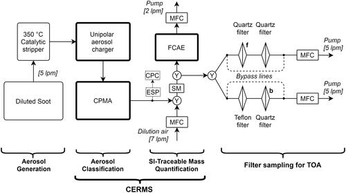
Following the stripper, particles were passed through a unipolar diffusion aerosol charger (UDAC, Cambustion, UK) to be charged for subsequent classification. The UDAC was operated at a charging level of $2\times {10}^{13}$ ions⋅ s⋅ m⁻³. Using a combination of condensation particle counter (CPC Model 3776, TSI, USA) and electrometer (Model E3068B, TSI Inc., USA) readings, we measured an average charge per particle between +6 and +14 for particles with mass-to-charge ratios between 0.2 fg/e and 1.0 fg/e, respectively, for the MISG burner. This trend reflects the fact that larger particles accumulate more charge for a given set of conditions (Reavell, Symonds, and Biskos 2004). (Note that these values are a function of the sampled size distribution, which influences the fractions of multiply charged particles transmitted by the CPMA at a given mass-to-charge setpoint.) By placing an electrostatic precipitator (ESP, Cambustion, UK) upstream of a CPC, we measured that zero particles remained uncharged after the UDAC.

Following the UDAC, particles were classified by mass-to-charge ratio using a CPMA (U111, Cambustion, UK). The CPMA was operated at a mass resolution of 2.5 (the inverse of the normalized full-width half maximum) for all MISG- and NRC-IFB measurements, and 2 or 3 for the miniCAST burner. These resolutions are slightly lower than typical operation for the CPMA used in a CERMS (typically >4; Dickau et al. 2015) but were adequate. (Note that a mass resolution of 3 would correspond to a size resolution of 9 if our experiment had involved classifying spheres.) The CPMA was operated in this manner to achieve manageable sampling times for the TOA filters. Lower resolutions can potentially increase the bias of the CERMS (Symonds, Reavell, and Olfert 2013); however, the results discussed below indicate that any potential bias was negligible. The MISG, NRC-IFB, and miniCAST soot was selected at mass-to-charge ratios of 0.2, 0.1, and 0.22 fg/e, respectively in order to maximize the PM mass concentration measured downstream. We reiterate that since these values are mass-to-charge ratios, they should not be mistaken as implying a median particle mass of 0.1–0.22 fg. The CPMA was warmed up for at least 1 h at the start of each experiment to allow its internal temperature to stabilize.

The CPMA was followed by a wye-splitter (9.525 mm inner diameter) which facilitated the addition of dilution air to the sample flow. This dilution was used to minimize the sample flow through the CPMA, which directly affects the CPMA resolution, while providing sufficient flow to the downstream instruments. A static mixer (Model 3/8-40-3-12-2, Koflo Corporation, IL, USA; labeled SM in Figure 1) installed after this wye splitter ensured that the sample and dilution flows were thoroughly mixed before flowing through the subsequent wye-splitter toward the instruments (Figure 1), as validated previously (Titosky et al. 2019).

After the static mixer, a second wye-splitter passed particles to a Faraday cup aerosol electrometer (FCAE, Model E3068B, TSI Inc., USA) and to a filter-sampling apparatus described below. The E3068B FCAE is an improvement to the aerosol electrometer used in the NRC CERMS in previous studies (Dickau et al. 2015; Titosky et al. 2019) and was tested as part of this study. Complete details are provided in the Appendix. We found that the baseline change after exposure to high particle concentrations was negligible. Using Allan variance analysis, we found that any drift in the bias of the instrument occurred slowly (i.e., measurements from the FCAE could be averaged for up to 40 min to improve measurement precision), although the precision at 1 Hz (i.e., no averaging) was smaller than the calibration accuracy of 1.2%. This quoted accuracy of 1.2% corresponds to the maximum bias observed during the calibration of our electrometer by the manufacturer. The uncertainty of this FCAE is therefore limited by the accuracy of its calibration at present. These results are consistent with a recent study by multiple national metrology institutes (Högström et al. 2014).

The internal MFC of our FCAE was not used during this study due to its guaranteed accuracy being only ± 5% at 2 to 10 SLPM (101.325 kPa and 273 K). (However, we note that the manufacturer’s calibration data indicated an accuracy of 2% or better.) Instead, an Alicat MC-5SLPM-D/5M MFC was used, with an accuracy of ± 0.8% of reading plus 0.2% of full scale, and repeatability ± 0.2% of full scale. This flow controller was operated in volumetric control mode.

The system described above (UDAC-CPMA-FCAE) and its careful configuration in terms of dilution, sampling lines, and flow verification comprises the NRC CERMS.

3.3. Filter sampling and thermal–optical analysis for EC, OC

A filter-sampling apparatus placed after the CPMA and shown in Figure 1 was used to obtain samples for TOA. Stainless steel filter holders (Pall Corporation, NY, USA, Part Number 1209) were used to sample onto the 25 mm-diameter filters specified below. To achieve a target mass density of >10 µg C cm⁻² on the filter at our flow rate of 5 SLPM, we sampled for durations ranging from 30 min to 8 h (median 65 min) according to the source concentration.

Filters were analyzed by TOA using the EUSAAR2 protocol (Cavalli et al. 2010) in a Sunset Laboratories Carbon Analyzer (model 5 L) (Birch and Cary 1996; Bauer et al. 2009). Inspection of the thermograms indicated that the majority of carbon evolved in the first or second stage of the protocol (that is, below 300 °C) and that pyrolyzed carbon was negligible, which suggests that our choice of protocol will have had little effect on our results.

For each test point, a 25 mm quartz filter (TISSUQUARTZ-2500-QAT-UP, Pall Corporation, NY, USA) was used to collect PM for analysis. As this filter will have adsorbed or absorbed significant amounts of gas-phase VOCs, a second quartz filter was also analyzed by TOA to measure and subtract these artifacts from the first (Subramanian et al. 2004). This second filter was not placed behind the quartz filter, since that filter has already removed some gas-phase VOCs (and could serve as a source of gas-phase VOCs under conditions where condensed-phase VOC evaporation was significant), but rather behind a 25 mm polytetrafluoroethylene (PTFE, sold as Teflon) filter (Zefluor P5PJ047, Pall Corporation, NY, USA), which should interact negligibly with gas-phase VOCs. To equalize the pressure drops across the analyzed filters, an additional quartz filter was placed behind the PM-loaded quartz filter. Neither this additional filter nor the PTFE filter was analyzed by TOA.

The filter sampling procedure was as follows. Quartz filters were pre-fired in-house at 900 °C for 6 h. The filters were handled with tweezers and the filter holders were handled only with gloves, avoiding direct contact with their interiors even with gloved hands. The flow through each pair of filters was controlled with two MFCs (Model MCRW-55LPM-D, Alicat Scientific, AZ, USA). At a given MFC setpoint, we found that the volumetric flow rates through each of the filter bypass lines (shown in Figure 1) varied significantly from day to day (maximally 7% and 4% of the mean for each line). This uncertainty would have propagated as the same percentage uncertainty in the calculated TOA-based mass concentrations. Therefore, for each measurement point reported herein, we first loaded 4 filters into the holder, then measured and set the volumetric flow through these filters using a bubble flow calibrator (Gilian Gilibrator 2, Sensidyne, FL, USA; accuracy better than 1%). We then discarded and replaced all 4 filters before beginning the measurement. This procedure is intended to account for day-to-day variability in the mass- to volumetric-flow conversion (due to ambient conditions), and does not account for variability in filter flow resistance.

In addition to the four filters sampled for each test point, sets of blank filters were taken. For these blanks, the entire sampling procedure was followed as usual except zero flow was passed through the filters (that is, blanks were equivalent to samples except that the sampling duration was zero seconds).

TOA provides a mass density of carbon on the filter, which can be converted to mean PM concentration of carbon during sampling $M_{\text{TC}}$ via (2) $$M_{\text{TC}}=\frac{A_{\text{filter}}{D}_{\text{TC}}}{Q\mathrm{\Delta }t}$$(2) where $A_{\text{filter}}$ [in units of cm²] is the exposed area of the filter during sampling; $D_{\text{TC}}$ [µg C cm⁻²] is the blank-subtracted area density of TC on the filter, as measured by TOA; $Q$ [cm³ s⁻¹] is the volumetric flow rate through the filter; and $\mathrm{\Delta }t$ [s] is the sampling duration.

In Equation (2)(2) $$M_{\text{TC}}=\frac{A_{\text{filter}}{D}_{\text{TC}}}{Q\mathrm{\Delta }t}$$(2) , $D_{\text{TC}}$ must be corrected for blank signals (see above) and VOC artifacts. VOC artifacts occur due to the evaporation of condensed-phase VOCs (loss of “true” OC signals) as well as the condensation of gas-phase VOCs due to adsorption and absorption (addition of “false” OC signals), and their quantification was discussed in the Background section. $D_{\text{TC}}$ is corrected prior to calculating $M_{\text{TC}}$ since these partitioning effects are typically independent of $Q$ and $\mathrm{\Delta }t.$ Thus VOC artifacts do not increase proportionally with PM concentrations, but rather approach asymptotic values.

Overall, the VOC-partitioning correction to $D_{\text{TC}}$ is $$X_{\text{VOC}}=\frac{D_{\text{OC},\mathrm{ }\text{fz}}+\left(D_{\text{OC},\mathrm{ }\mathrm{b}}-D_{\text{OC},\mathrm{ }\text{bz}}\right)}{{D_{\mathrm{EC}}+D}_{\text{OC},\mathrm{f}}}\mathrm{ }\left(3\mathrm{a}\right)$$ where the subscript letters f and b represent the front and back filters labeled in Figure 1, and the subscript z indicates $\mathrm{\Delta }t$ of zero for these filters. The measured values of $X_{\text{VOC}}$ in this work are given in Table 2. The magnitude of this correction influences the accuracy of a calculated EC mass concentration.

Table 2. Properties of the soot generated and used in this study.

Soot source	No. of filters	EC/TC [−]	VOC-partitioning correction to TC^a [%]	Carbon mass fraction^b $f_C$ [%]
MISG	6	0.96 ± 0.02	38 ± 2	92.7 ± 0.7
miniCAST	3	0.81 ± 0.06	25 ± 1	n.d.^c
NRC-IFB	4	0.83 ± 0.08	40 ± 2	90.0 ± 0.1

Each reported property is the mean and standard error of the mean, for all measurements.

^a Defined by Equation (3)$$X_{\text{VOC}}=\frac{D_{\text{OC},\mathrm{ }\text{fz}}+\left(D_{\text{OC},\mathrm{ }\mathrm{b}}-D_{\text{OC},\mathrm{ }\text{bz}}\right)}{{D_{\mathrm{EC}}+D}_{\text{OC},\mathrm{f}}}\mathrm{ }\left(3\mathrm{a}\right)$$ and representing back-filter OC plus blank-filter OC, divided by TC (see Equation (3)$$X_{\text{VOC}}=\frac{D_{\text{OC},\mathrm{ }\text{fz}}+\left(D_{\text{OC},\mathrm{ }\mathrm{b}}-D_{\text{OC},\mathrm{ }\text{bz}}\right)}{{D_{\mathrm{EC}}+D}_{\text{OC},\mathrm{f}}}\mathrm{ }\left(3\mathrm{a}\right)$$).

^b Measured either by elemental or gravimetric-plus-TOA analysis.

^c Not determined (n.d.) for miniCAST soot, where the average of the MISG and NRC-IFB values was used (91.4 ± 2.7%). The high VOC-partitioning corrections for the MISG in this study are in contrast to those reported by Moallemi et al. (2019) for the same burner, and partly reflect the fact that much less dilution was used in this study due to the high concentrations required for filter sampling.

The magnitude of $D_{\text{TC}}$ after VOC-partitioning correct is given by $$D_{\text{TC},\text{corrected}}=D_{\text{EC}}+D_{\text{OC},\text{corrected}}=D_{\text{EC}}+D_{\text{OC},\mathrm{f}}-D_{\text{OC},\text{fz}}-\left(D_{\text{OC},\mathrm{ }\mathrm{b}}-D_{\text{OC},\mathrm{ }\text{bz}}\right)\mathrm{ }{(D}_{\text{TC},\text{uncorr}}\left)\right(1-X_{\mathrm{VOC}}\left)\mathrm{ }\right(3\mathrm{b})$$

In practice, blank filters contain OC but not EC, so $D_{\text{OC},\text{fz}}$ and $D_{\mathrm{OC},\mathrm{bz}}$ are obtained from the TC measured on the blank filters. $D_{\text{EC}}$ and $D_{\text{OC},\text{front}-\text{filter}}$ are determined from $D_{\text{TC},\text{front}-\text{filter}}$ according to the OC/EC split point determined by TOA.

3.4. CERMS PM mass concentration

The CERMS measures PM mass concentration $M_{\text{PM}}$ via the number of charged particles per second that reach an electrometer to generate an electrical current $I,$ (4) $$M_{\text{PM}}=\frac{m_{1}I}{Qe}$$(4) where $m_1$ is the setpoint of a CPMA upstream of the detector, $Q$ is the volumetric flow rate to the detector, and $e$ is the elementary charge (Symonds, Reavell, and Olfert 2013).

Since the CPMA classifies particles by mass-to-charge ratio, independently of any other physical parameters, Equation (4)(4) $$M_{\text{PM}}=\frac{m_{1}I}{Qe}$$(4) holds for both singly- and multiply charged particles. Equation (4)(4) $$M_{\text{PM}}=\frac{m_{1}I}{Qe}$$(4) only requires that the number of uncharged particles is negligible, a condition which we routinely confirmed by measuring uncharged particles number concentrations with a CPC (Model 3776, TSI, USA) placed behind an electrostatic precipitator (ESP, Cambustion, UK).

3.5. Comparing TOA and CERMS mass concentrations

Total PM mass concentration $M_{\text{PM}}$ can be compared to TC mass concentration $M_{\text{TC}}$ via (5) $$M_{\text{PM}}=\frac{M_{\text{TC}}}{f_{\mathrm{c}}}$$(5) where $M_{\text{TC}}$ is the mass concentration of carbon measured by TOA (Equation (2)(2) $$M_{\text{TC}}=\frac{A_{\text{filter}}{D}_{\text{TC}}}{Q\mathrm{\Delta }t}$$(2) ) and $f_{\mathrm{C}}$ is the mass fraction of carbon in the PM. Conversely, for the EC-based calibration of instruments using $M_{\text{PM}}$ (e.g., as measured by the CERMS), $M_{\text{EC},\mathrm{ }\text{CERMS}}$ can be calculated as (6) $$M_{\mathrm{EC},\mathrm{CERMS}}=M_{\mathrm{PM},\mathrm{CERMS}}\cdot \left(\mathrm{EC}/\mathrm{TC}\right)\cdot f_{\mathrm{C}}$$(6)

The quantity EC/TC must be measured by a standard TOA method, because EC is defined only by TOA and does not uniquely nor robustly correlate with the mass of any well-defined material. Thus, although BC instruments can be directly calibrated with the CERMS using the nonvolatile fraction of soot (Dickau et al. 2015), any calibration which defines EC as its reference must include a TOA measurement of this operationally defined quantity. The EC/TC of a given calibration source is a characteristic of that source, and need only be checked periodically rather than measured for each calibration point.

In Equations (5)(5) $$M_{\text{PM}}=\frac{M_{\text{TC}}}{f_{\mathrm{c}}}$$(5) and (6)(6) $$M_{\mathrm{EC},\mathrm{CERMS}}=M_{\mathrm{PM},\mathrm{CERMS}}\cdot \left(\mathrm{EC}/\mathrm{TC}\right)\cdot f_{\mathrm{C}}$$(6) , the mass fraction of carbon $f_{\mathrm{C}}$ converts from total PM mass to carbonaceous mass, and can be measured directly by standard analytical techniques. For the routine application of the methodology presented here, we recommend determining $f_{\mathrm{C}}$ using $M_{\text{PM}}$ from gravimetric analysis and $M_{\text{TC}}$ from TOA.

In the present study, we have measured $f_{\mathrm{C}}$ using an independent method (elemental analysis; EA) since our goal is to demonstrate closure between the CERMS and TOA. We therefore collected a soot sample on a Teflon membrane filter, transferred the filtered sample to a glass vial, and measured its elemental content with a Vario ISOTOPE cube (Elementar Analysensysteme GmbH, Germany). Potential contamination from the vial was minimized by pre-heating the vial and its cap for 3 h at 100 °C. This instrument combusts a pre-weighed bulk soot sample in oxygen and ultra-pure helium and measures the resulting gases using a thermal conductivity detector. The fundamental principles by which we measured $f_{\mathrm{C}}$ are therefore comparable to the gravimetric-plus-TOA approach described above.

It is illustrative to relate $f_{\mathrm{C}}$ to the common TOA-related quantity OM/OC (mass ratio of organic PM to organic carbon). The OM/OC is typically used in the TOA community to convert OC mass to organic PM mass, $M_{\text{OM}}.$ This $M_{\text{OM}}$ accounts for the hydrogen, oxygen, or other atoms present within organic molecules, which contribute an additional 20–60% to $M_{\text{OM}}$ relative to $M_{\text{TC}},$ corresponding to an OM/OC of 1.2 to 2.1 (Turpin and Lim 2001; Bae, Schauer, and Turner 2006).

$f_{\mathrm{C}}$ is related to OM/OC via (7) $$\frac{1}{f_{\mathrm{C}}}=\frac{M_{\text{PM}}}{M_{\text{TC}}}=\frac{M_{\mathrm{C}}+M_{\mathrm{H}}+M_{\mathrm{O}}+M_{\mathrm{X}}}{M_{\text{TC}}}=\frac{M_{\text{OC}}+M_{\text{EC}}+M_{\mathrm{H}}+M_{\mathrm{O}}+M_{\mathrm{X}}}{M_{\text{OC}}+M_{\text{EC}}}=\left(\frac{\text{EC}}{\text{TC}}\right)+\frac{M_{\text{OM}}+M_{\mathrm{H}-\text{in}-\text{BC}}+M_{\mathrm{O}-\text{in}-\text{BC}}+M_{\mathrm{X}}}{M_{\text{OC}}+M_{\text{EC}}}$$(7) where $M_{\mathrm{C}},$ $M_{\mathrm{H}},\mathrm{ }{M}_{\mathrm{O}},$ and $M_{\mathrm{X}}$ are the masses of carbon, hydrogen, oxygen, and other atoms in the PM sample. The quantities $M_{\mathrm{H}-\text{in}-\text{BC}}$ and $M_{\mathrm{O}-\text{in}-\text{BC}}$ are the masses of hydrogen and oxygen associated with BC. (These are referred to as “in-BC” and not “in-EC”, since the definition of EC excludes non-carbon-mass.) The quantity $M_{\mathrm{X}}$ is often negligible, since the distillate fuels used for on-road vehicles and aircraft turbine engines contain only trace amounts of impurities. For fuels containing biomass or crude-oil residual, $M_{\mathrm{X}}\mathrm{ }$ may include sulfur, metals, the oxygen in metal oxides, and salts such as potassium chloride; for such fuels $M_{\mathrm{X}}$ may contribute a significant fraction of $M_{\text{PM}}$ mass when the combustion efficiency is high (e.g., Torvela et al. 2014).

The quantities $M_{\mathrm{H}-\text{in}-\text{BC}}$ and $M_{\mathrm{O}-\text{in}-\text{BC}}$ are non-zero due to BC surface functionalities such as hydroxyl or carbonyl groups (Matuschek et al. 2007; Corbin et al. 2015) or due to internal hydrogen in less mature soot (Michelsen 2017). $M_{\mathrm{H}-\text{in}-\mathrm{B}\mathrm{C}}$ is typically negligible; although C/H elemental ratios are typically 10–20 (Michelsen 2017), the low atomic mass of hydrogen means that it contributes under 1% of the BC mass. In contrast, the high atomic mass of oxygen means that $M_{\mathrm{O}-\mathrm{i}\mathrm{n}-\mathrm{B}\mathrm{C}}$ is much more substantial, contributing approximately 2–10% of the overall BC mass (Figueiredo et al. 1999; Singh and Vander Wal 2020). This corresponds to an approximate $f_{\mathrm{C}}$ of 0.9 for BC. PM samples which also include non-BC material may have lower $f_C.$ For example, the $f_{\mathrm{C}}$ of a PM sample may be lower according to the mass fraction of $M_{\mathrm{OM}}$ in the sample: since $f_{\mathrm{C}}\to {\left(\text{OM}/\text{OC}\right)}^{-1}$ as $\text{EC}\to 0,$ a pure OM sample may have $f_{\mathrm{C}}$ as low as 0.5 for an OM/OC of 2.0.

In this study, our measurements of $f_{\mathrm{C}}$ implicitly account for $M_{\mathrm{H}-\text{in}-\text{BC}}$ and $M_{\mathrm{O}-\text{in}-\text{BC}}$ and for the mass fraction of $M_{\mathrm{OM}}$ in our samples.

3.6. Uncertainties

TOA uncertainties were calculated according to the manufacturer’s recommendations for the area density of carbon on the filter, followed by propagation of error through Equation (2)(2) $$M_{\text{TC}}=\frac{A_{\text{filter}}{D}_{\text{TC}}}{Q\mathrm{\Delta }t}$$(2) . The manufacturer’s recommendations include both a proportional and absolute error term, representing relative precision and absolute precision, respectively (Rocke and Lorenzato 1995); these two terms were added in quadrature.

CERMS uncertainties were calculated based on the intermediate precision of 2.1% given by Titosky et al. (2019). This proportional term was combined in quadrature with an absolute uncertainty of 0.1 µg m⁻³, which was conservatively calculated using 10 times the maximum standard deviation of the observed current (0.3 fA) in several blank experiments, where a filter was placed on the FCAE following high-concentration measurements. Uncertainties in all calculated quantities were estimated by simple error propagation.

4. Results

4.1. Closure between CERMS and EC

Table 2 presents the properties of the soot particles generated in this study. The MISG, miniCAST, and NRC-IFB soot particles had mean EC/TC ratios of 0.96 ± 0.02, 0.81 ± 0.06, and 0.83 ± 0.08 (uncertainties are 1σ of the standard error), respectively. These ratios have already been corrected for gas-phase VOC-related artifacts (Equation (3a)$$X_{\text{VOC}}=\frac{D_{\text{OC},\mathrm{ }\text{fz}}+\left(D_{\text{OC},\mathrm{ }\mathrm{b}}-D_{\text{OC},\mathrm{ }\text{bz}}\right)}{{D_{\mathrm{EC}}+D}_{\text{OC},\mathrm{f}}}\mathrm{ }\left(3\mathrm{a}\right)$$); the magnitude of this correction was 38 ± 2%, 25 ± 1%, and 40 ± 2% of TC for the respective burners.

The measured carbon mass fraction $f_{\mathrm{C}}$ for MISG soot was 92.7 ± 0.7%. For NRC-IFB soot, this value was 90.0 ± 0.1%. The $f_{\mathrm{C}}$ measurements were unavailable for CAST soot, so the mean of the MISG and NRC-IFB values was used: 91.4 ± 2.7%. Since only three CAST measurements were included in this study and since the two measured values were different by only 3.7%, we have treated the additional uncertainty due to this extrapolation as negligible.

Figure 2 summarizes the main results of this work. The plot abscissa is the PM mass concentration measured by the CERMS, $M_{\text{PM}-\text{CERMS}},$ which is taken as a reference since the uncertainties of the CERMS are well-constrained and low (repeatability of 1.1% and intermediate precision of 2.1%; Titosky et al. 2019). The measured $M_{\text{PM}-\text{CERMS}}$ varies from 13 to 240 µg m⁻³. The plot ordinate is the PM mass concentration measured by TOA–Elemental-Analysis, $M_{\text{PM}-\text{TOA}-\mathrm{E}\text{lem}-\mathrm{A}\text{nal}},$ the mass concentration of PM determined by TOA after using the elemental analysis results to correct for the fact that total carbon (measured by TOA) is not equal to total PM mass (Equation (5)(5) $$M_{\text{PM}}=\frac{M_{\text{TC}}}{f_{\mathrm{c}}}$$(5) ).

Figure 2. Comparison of PM mass determined by TOA–Elemental-Analysis and by CERMS. Error bars show one standard error. Fit is uncertainty-weighted least-squares minimization; fit uncertainties show 95% confidence intervals. The fitted slope and intercept are not significantly different from one and zero, respectively, indicating agreement between the two techniques.

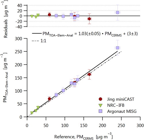
According to the fit in Figure 2, there is no significant difference between the PM mass concentrations determined by TOA–Elemental-Analysis or by the CERMS for our data. This mass closure demonstrates that our understanding of the two systems is adequate and implies that an instrument calibrated by either approach would report the same mass concentrations thereafter.

In Figure 2, the data have been fitted by uncertainty-weighted least-squares minimization. Repeating the fit to exclude the CAST soot data (for which $f_{\mathrm{C}}$ was not measured directly) resulted in no substantial change in the result. The resulting residuals show no distinguishable difference in the results for the different soot sources. The residuals do show some heteroscedasticity; this implies that our measurement precision was proportional to the measured signal and therefore that our measurement repeatability in one of the parameters required to calculate $M_{\text{PM}-\text{TOA}-\mathrm{E}\text{lem}-\mathrm{A}\text{nal}}$ limited our overall precision. We suspect that our flow rate measurements, including flow through the TOA filters, are the most likely cause of this uncertainty. The fact that our CPMA was operated at a lower-than normal resolution, due to the high concentrations required for the TOA filters, would not have contributed to this scatter, since resolution limitations would have resulted in systematic, source-specific biases rather than concentration-dependent scatter. The fact that no systematic biases were observed demonstrates that our uncertainties were dominated by random error. As the residuals appear to be randomly distributed as a function of concentration for each source, this bias and any other potential biases were negligible relative to random errors.

4.2. Application of CERMS to instrument calibration at low concentrations

To demonstrate the advantage of the CERMS calibration approach over TOA EC, we present two different applications in Figures 3 and 4.

4.2.1. Evaluation of LII 300 limit of detection

Figure 3 shows the calibration of an Artium LII 300 laser-induced incandescence instrument at concentrations ranging from 0.37 to 15.9 µg m⁻³ (see Dickau et al. 2015 for a calibration at concentrations up to 170 µg m⁻³) using a setup identical to that shown in Figure 1, except for the following changes: the MISG soot was diluted by a Dekati ejector dilutor, the filter sampling apparatus was replaced with an LII 300, and the flows of dilution air, FCAE, and LII 300 were all set to 4 SLPM. The calibration fit was performed as in Figure 2 and the residuals are shown on the upper panel. The LII 300 demonstrated linearity within ±0.2 µg m⁻³ over the concentration range of this calibration.

Figure 3. Demonstration of CERMS-based EC calibration at low concentrations using an Artium LII 300 instrument. The filter sampling apparatus in Figure 1 was replaced with the LII 300 for this experiment. Calibration was performed with (red circles) and without (black triangles) catalytic stripper. Inset shows the lowest measured concentrations and 0.35 µg m⁻³ minimum value reported by the LII 300. The dotted line labeled “TOA” represents a filter-based TOA calibration sample taken at 2470 µg m⁻³ over 5 min. At the lowest concentration used for the CERMS calibration (0.2 µg m⁻³), a filter would have required >17 days of sampling.

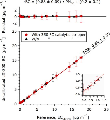
The calibration (red circles) includes 12 points measured over 80 min. The calibration was additionally repeated without the catalytic stripper (black triangles), which gave an identical result, and demonstrated that this catalytic stripper was superfluous for diluted MISG soot. The stripper may nevertheless be necessary for other sources which produce higher VOC mass fractions.

The calibration fit in Figure 3 reports a 0.2 µg m⁻³ intercept. As shown by the figure inset, this corresponds to a deviation of the LII 300 data toward a minimum reported value of 0.35 µg m⁻³. This deviation is at least partly due to the fact that the LII 300 reports no values, rather than zeroes or negative concentrations for signals below its limit of detection. The result is that low signals cannot and do not average to zero. The CERMS data show that this bias only occurs at low concentrations, and indicate the minimum value at which this issue arises. According to this bias, measurements from this LII 300 should be carefully inspected at low concentrations, and, for a minimum accuracy of 20%, rejected below 1 µg m⁻³. This limit may be relaxed if the user is willing to accept greater uncertainty.

This low-concentration calibration would not have been practically possible with a TOA-based calibration: at the lowest concentration used for the CERMS calibration (0.2 µg m–3), a single filter would have required >17 days of sampling. In contrast, the CERMS sampling and analysis time is independent of concentration.

4.2.2. Evaluation of photoacoustic calibration

The photoacoustic extinctiometer (PAX; Droplet Measurement Technologies, USA) is normally calibrated using the Beer-Lambert law by reference to its internal laser power meter. The use of the Beer-Lambert law requires concentrations high enough to significantly attenuate the PAX laser power ($\gg 1000$ µg m⁻³), and the calibration is then extrapolated to lower values without validation.

Using the CERMS, we evaluated the calibration of a PAX down to its limit of detection, as shown in Figure 4. For this experiment, an alternative CERMS configuration was employed: a 3 liter sample reservoir was added upstream of the UDAC and CPMA, the reservoir was filled with MISG soot, then a filter was added before the reservoir to allow gradual dilution by either filtered flame smoke or filtered laboratory air. This fill/dilution cycle was repeated 3 times, in the runs labeled A, B, and C. The FCAE and PAX flows were each 1.2 SLPM and no post-CPMA dilution flow was used. The CERMS data were used to calculate equivalent EC mass using Equation (6)(6) $$M_{\mathrm{EC},\mathrm{CERMS}}=M_{\mathrm{PM},\mathrm{CERMS}}\cdot \left(\mathrm{EC}/\mathrm{TC}\right)\cdot f_{\mathrm{C}}$$(6) , as in Section 4.1.

Figure 4. Demonstration of the CERMS as a reference measurement for determining the linearity of an optically calibrated photoacoustic spectrometer (PAX). The PAX optical calibration is performed at extremely high concentrations (green triangle), and is normally extrapolated to zero without quantification of its lower limit of detection (LOD). The CERMS data show that this extrapolation is valid for concentrations down to a few µg m⁻³, with a lower limit strongly dependent on the stability of the relative humidity (RH) of the gas. The upper panel shows the ratio of the PAX- and CERMS-reported mass concentrations, which could be used to calculate a mass absorption coefficient.

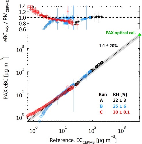
Figure 4 shows that the PAX-reported eBC (after Beer-Lambert-law calibration) was accurate to within a few percentage of the CERMS mass concentration for most concentrations. This accuracy depends not only on the accuracy of the PAX calibration, but also on the accuracy of the mass-absorption efficiency (MAE), also called mass absorption cross-section (MAC), used by the PAX to convert from measured light absorption coefficients to equivalent BC mass concentration. For this conversion, the PAX uses the MAE recommended by Bond et al. (2013). The MISG produces soot with a similar MAE (Moallemi et al. 2019).

The excellent correlation between PAX and EC_CERMS in Figure 4 confirms the extrapolation of the PAX calibration from approximately 4000 µg m⁻³ down to approximately 5 µg m⁻³. However, below 5 µg m⁻³, the correlation breaks down. This can be explained by differences in the trend of relative humidity (RH) during the measurements. During Runs A and B, laboratory air was used to dilute the sample, which was dryer than the sample aerosol, and led to variability in the sample RH and therefore deviation from the 1:1 line. During Run C, diluted sample aerosol was used, which stabilized the RH and allowed the PAX to remain accurate to within 20% of 1:1 down to 2 µg m⁻³, and accurate to within 50% of 1:1 down to 1 µg m⁻³.

Our use of an alternative CERMS configuration in these experiments was intentionally chosen to illustrate the importance of these slow RH changes. Note that, unlike for the LII 300 results above, the measured PAX accuracy is not generalizable since variability in RH is sample dependent. Moreover, an RH sensor cannot be used to compensate for this variability, as the variability may be non-linear due to the effects of RH on the photoacoustic efficiency (Gillis, Havey, and Hodges 2010) or microphone performance.

5. Discussion and conclusions

Our experimental demonstration of consistency between TOA and CERMS measurements supports the application of the recently developed CERMS approach to the calibration of BC mass instruments. For calibrations which previously relied upon TOA-defined EC, the CERMS method provides real-time data and avoids the VOC-related artifacts which occur during TOA sampling. Moreover, the CERMS method reports PM mass concentrations every second, can be operated at flows less than 1 SLPM, and (as shown by Titosky et al. 2019) has a much better repeatability and intermediate precision than TOA.

The PM mass concentration determined by CERMS is a physically traceable and precisely defined quantity, unlike the EC mass concentration defined by TOA. Such a clear definition of PM mass concentration may help reduce ambiguity in the interpretation of different “EC” or “BC” measurement techniques (Petzold et al. 2013) which are sensitive to such effects as gas-phase VOC adsorption and absorption onto filters, catalytic decomposition by metal compounds or sulfates, or morphological effects. The CERMS avoids these complications by measuring the total PM mass (of BC or any other nonvolatile material) directly. If a reference BC aerosol is generated from a well-characterized source, for example, by removing volatiles from flame or engine soot, then BC mass instruments can be calibrated via the CERMS without any need for filter sampling. In this case, the calibration is to a reference BC material rather than to TOA-defined EC. Because TOA EC does not include the entire mass of the reference BC particles (in other words, because $f_C<1$ and EC/TC $<1$ in Equation (6)(6) $$M_{\mathrm{EC},\mathrm{CERMS}}=M_{\mathrm{PM},\mathrm{CERMS}}\cdot \left(\mathrm{EC}/\mathrm{TC}\right)\cdot f_{\mathrm{C}}$$(6) and Table 2) a reference-BC calibration factor will be slightly different to an EC-based calibration factor.

The characterization of a source of reference-BC particles should include measurements of $f_{\mathrm{C}}$ and EC/TC, which provide, for example, information on the elemental composition of the sample and context with literature, respectively. Using these measurements, BC instruments may be calibrated to EC as necessary, instead of to total soot mass. In both cases, a CERMS-based calibration will provide a much larger number of calibration points than a TOA-based calibration, and will therefore provide a more statistically robust result in a much shorter time than required for TOA analysis.

Acknowledgments

The technical assistance of Simon-Alexandre Lussier with the filter sampling, Daniel Clavel with the LII calibration, and Brett Smith with the TOA analysis were essential to this work. We thank the G. G. Hatch Isotope Laboratory of the University of Ottawa for elemental analysis of our soot samples.

Additional information

Funding

This work was partially funded by the Office of Energy Research and Development (OERD) of Natural Resources Canada (NRCan), grant EIP-EU-TR3-04, and by Transport Canada.

Appendix:

CERMS electrometer performance

This appendix presents experiments performed to characterize the new 3068B FCAE of the NRC CERMS. In some cases, we compare the 3068B to our previous FCAE configuration (Dickau et al. 2015; Titosky et al. 2019), which consisted of a Faraday cup fabricated in-house, combined with a commercial electrometer (Keithley 6514, Keithley, USA).

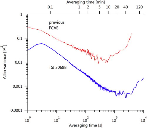
Figure A1 shows calibration data and residuals for the 3068B FCAE used in this work. Calibration was performed by the manufacturer. Figure A2 shows an Allan variance analysis of both the new and former FCAEs. The 3068B displays over an order of magnitude less noise, and may be averaged for up to 1000s for increased precision. However, the calibration accuracy of 5 fA (manufacturer value) is an order of magnitude higher than the Allan variance of 0.02 fA at 1 s averaging times; calibration accuracy therefore limits FCAE uncertainty.

Figure A1. Calibration data for the 3068B FCAE. Upper panel shows percent residuals.

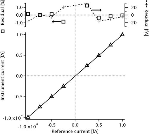
Figure A2. Allan variance plots of the previous FCAE (Keithley-plus-in-house FCAE) and TSI 3068B FCAE configurations. The sample data represent multiple hours of measurements on filtered laboratory air. The maximum Allan variance, up to 120 min, is much smaller than the electrometer calibration uncertainties shown in Figure A1.

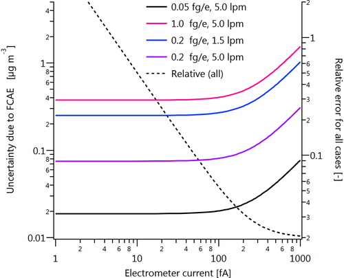
Figure A3 illustrates the uncertainty contributed to the CERMS by the FCAE for a variety of conditions. Uncertainties were calculated as (A1) $${\delta }_{\text{FCAE}}=\sqrt{{\sigma }_{\text{calibration}}^2+{\left(0.02I\right)}^2+{\sigma }_{3068\mathrm{B}}^2\mathrm{}}$$(A1) where ${\sigma }_{\text{calibration}}$ is the uncertainty in the calibration of electrometer current and $0.02I$ is 2% of the FCAE current; these two terms are the uncertainty terms recommended by the manufacturer. The additional term ${\sigma }_{3068\mathrm{B}}$ is the precision in electrometer current estimated from the standard deviation of measurements on filtered laboratory air and equal to 0.3 fA. Equation (A1)(A1) $${\delta }_{\text{FCAE}}=\sqrt{{\sigma }_{\text{calibration}}^2+{\left(0.02I\right)}^2+{\sigma }_{3068\mathrm{B}}^2\mathrm{}}$$(A1) does not account for uncertainties in flow-rate measurements ($Q$ in Equation (1)(1) $$M_{\text{classified}}=\sum _{i=1}^k{N}_i\cdot i{m}_1=\frac{m_{1}I}{Qe}$$(1) ); the reader is referred to Dickau et al. (2015) for related discussion.

Figure A3. Calculated uncertainties in mass concentration due to FCAE uncertainties according to Equation (A1)(A1) $${\delta }_{\text{FCAE}}=\sqrt{{\sigma }_{\text{calibration}}^2+{\left(0.02I\right)}^2+{\sigma }_{3068\mathrm{B}}^2\mathrm{}}$$(A1) for a range of FCAE flows and CPMA setpoints.

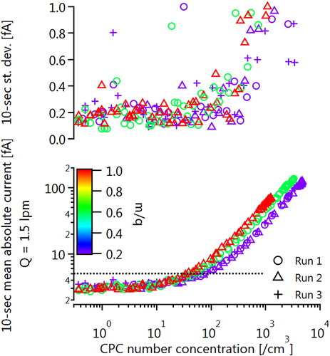
Figure A4 shows the 10-second-averaged mean and standard deviation of the TSI 3068B plotted against CPC number concentration, for a slowly decaying signal. The signal was produced by filling a 3 liter stainless steel vessel with sodium chloride particles and slowly diluting the vessel with compressed, filtered air. As the CPC was calibrated with the FCAE, was operated in single-particle counting mode, and therefore has a much lower limit of quantification than the FCAE, it served as a suitable reference for linearity. The CPMA was operated with m/q values of 0.2, 0.6, and 1.0 fg/e. The figure shows that linearity between the two detectors was maintained until the predicted accuracy of 5 fA was approached, at which point the FCAE signal began to tend toward its background value of 3 fA. This background was not subtracted from the data for this plot. The trends shown in Figure A4 therefore confirm that the FCAE behaves as expected near its detection limit.

Figure A4. Linearity of electrometer response demonstrated with a CPC for various $m/q$ setpoints at the CPMA. The background signal of about 3 fA was not subtracted from the FCAE data to better illustrate the trends.

References

- Aakko-Saksa, P., P. Koponen, M. Aurela, H. Vesala, P. Piimäkorpi, T. Murtonen, O. Sippula, H. Koponen, P. Karjalainen, N. Kuittinen, et al. 2018. Considerations in analysing elemental carbon from marine engine exhaust using residual, distillate and biofuels. J. Aerosol Sci. 126:191–204. doi: 10.1016/j.jaerosci.2018.09.005.
- Andreae, M., and A. Gelencsér. 2006. Black carbon or brown carbon? The nature of light-absorbing carbonaceous aerosols. Atmos. Chem. Phys. 6 (10):3131–48. doi: 10.5194/acp-6-3131-2006.
- Bae, M.-S., J. J. Schauer, and J. R. Turner. 2006. Estimation of the monthly average ratios of organic mass to organic carbon for fine particulate matter at an urban site. Aerosol Sci. Technol. 40 (12):1123–39. doi: 10.1080/02786820601004085.
- Bauer, J. J., X.-Y. Yu, R. Cary, N. Laulainen, and C. Berkowitz. 2009. Characterization of the sunset semi-continuous carbon aerosol analyzer. J. Air Waste Manag. Assoc. 59 (7):826–33. doi: 10.3155/1047-3289.59.7.826.
- Birch, M. E., and R. A. Cary. 1996. Elemental carbon-based method for monitoring occupational exposures to particulate diesel exhaust. Aerosol Sci. Technol. 25 (3):221–41. doi: 10.1080/02786829608965393.
- Bond, T. C., and R. W. Bergstrom. 2006. Light absorption by carbonaceous particles: An investigative review. Aerosol Sci. Technol. 40 (1):27–67. doi: 10.1080/02786820500421521.
- Bond, T. C., S. J. Doherty, D. W. Fahey, P. M. Forster, T. Berntsen, B. J. DeAngelo, M. G. Flanner, S. Ghan, B. Kärcher, D. Koch, et al. 2013. Bounding the role of black carbon in the climate system: A scientific assessment. J. Geophys. Res. Atmos. 118 (11):5380–552. doi: 10.1002/jgrd.50171.
- Boparai, P., J. Lee, and T. C. Bond. 2008. Revisiting Thermal-Optical Analyses of Carbonaceous Aerosol Using a Physical Model. Aerosol Sci. Technol. 42 (11):930–48. doi: 10.1080/02786820802360690.
- Burtscher, H. 2005. Physical characterization of particulate emissions from diesel engines: A review. J. Aerosol Sci. 36 (7):896–932. doi: 10.1016/j.jaerosci.2004.12.001.
- Cavalli, F., M. Viana, K. E. Yttri, J. Genberg, and J.-P. Putaud. 2010. Toward a standardised thermal-optical protocol for measuring atmospheric organic and elemental carbon: The EUSAAR protocol. Atmos. Meas. Tech. 3 (1):79–89. doi: 10.5194/amt-3-79-2010.
- Chow, J. C., J. G. Watson, L.-W A. Chen, M. O. Chang, N. F. Robinson, D. Trimble, and S. Kohl. 2007. The IMPROVE_a temperature protocol for thermal/optical carbon analysis: Maintaining consistency with a long-term database. J. Air Waste Manag. Assoc. 57 (9):1014–23. doi: 10.3155/1047-3289.57.9.1014.
- Coderre, A. R., K. A. Thomson, D. R. Snelling, and M. R. Johnson. 2011. Spectrally resolved light absorption properties of cooled soot from a methane flame. Appl. Phys. B 104 (1):175–88. doi: 10.1007/s00340-011-4448-9.
- Corbin, J. C., H. Czech, D. Massabo, F. Buatier de Mongeot, G. Jakobi, F. Liu, P. Lobo, C. Mennucci, A. A. Mensah, J. Orasche, et al. 2019. Refractory, infrared-absorbing carbon in ship exhaust from heavy fuel oil combustion. npj Atmos. Clim. Sci. 12 (2). doi:10.1038/s41612-019-0069-5
- Corbin, J. C., and M. Gysel-Beer. 2019. Detection of tar brown carbon with a single particle soot photometer (SP2). Atmos. Chem. Phys. 19 (24):15673–90. doi: 10.5194/acp-19-15673-2019.
- Corbin, J. C., U. Lohmann, B. Sierau, A. Keller, H. Burtscher, and A. A. Mensah. 2015. Black-carbon-surface oxidation and organic composition of beech-wood soot aerosols. Atmos. Chem. Phys. 15 (20):11885–907. doi: 10.5194/acp-15-11885-2015.
- Corbin, J. C., W. Peng, J. Yang, D. E. Sommer, U. Trivanovic, P. Kirchen, J. W. Miller, S. Rogak, D. R. Cocker, G. J. Smallwood, et al. 2020. Characterization of particulate matter emitted by a marine engine operated with liquefied natural gas and diesel fuels. Atmos. Environ. 220:117030. doi: 10.1016/j.atmosenv.2019.117030.
- Dickau, M., T. J. Johnson, K. Thomson, G. Smallwood, and J. S. Olfert. 2015. Demonstration of the CPMA-electrometer system for calibrating black carbon particulate mass instruments. Aerosol Sci. Technol. 49 (3):152–58. doi: 10.1080/02786826.2015.1010033.
- Durdina, L., P. Lobo, M. B. Trueblood, E. A. Black, S. Achterberg, D. E. Hagen, B. T. Brem, and J. Wang. 2016. Response of real-time black carbon mass instruments to mini-CAST soot. Aerosol Sci. Technol. 50 (9):906–18. doi: 10.1080/02786826.2016.1204423.
- Figueiredo, J. L., M. F. R. Pereira, M. M. A. Freitas, and J. J. M. Órfão. 1999. Modification of the surface chemistry of activated carbons. Carbon N. Y. 37 (9):1379–89. doi: 10.1016/S0008-6223(98)00333-9.
- Fung, K. 1990. Particulate carbon speciation by MnO2 oxidation. Aerosol Sci. Technol. 12 (1):122–27. doi: 10.1080/02786829008959332.
- Fung, K., J. C. Chow, and J. G. Watson. 2002. Evaluation of OC/EC speciation by thermal manganese dioxide oxidation and the IMPROVE method. J. Air Waste Manag. Assoc. 52 (11):1333–41. doi: 10.1080/10473289.2002.10470867.
- Gillis, K. A., D. K. Havey, and J. T. Hodges. 2010. Standard photoacoustic spectrometer: Model and validation using O2 A-band spectra. Rev. Sci. Instrum. 81 (6):064902. doi: 10.1063/1.3436660.
- Grahame, T. J., R. Klemm, and R. B. Schlesinger. 2014. Public health and components of particulate matter: The changing assessment of black carbon. J. Air Waste Manag. Assoc. 64 (6):620–60. doi: 10.1080/10962247.2014.912692.
- Guillemin, M., V. Perret, D. Dabill, R. Grosjean, D. Dahmann, and R. Hebisch. 2001. Further round-robin tests to improve the comparability between laboratories of the measurement of carbon in diesel soot and in environmental samples. Int. Arch. Occup. Environ. Health 74 (2):139–47. doi: 10.1007/s004200000194.
- Hand, J. L., W. C. Malm, A. Laskin, D. Day, T. Lee, C. Wang, C. Carrico, J. Carrillo, J. P. Cowin, J. Collett, and M. J. Iedema. 2005. Optical, physical, and chemical properties of tar balls observed during the Yosemite Aerosol Characterization Study. J. Geophys. Res. 110 (D21):D21210. doi: 10.1029/2004JD005728.
- Hebisch, R., D. Dabill, D. Dahmann, F. Diebold, N. Geiregat, R. Grosjean, M. Mattenklott, V. Perret, and M. Guillemin. 2003. Sampling and analysis of carbon in diesel exhaust particulates-an international comparison. Int. Arch. Occup. Environ. Health 76 (2):137–42. doi: 10.1007/s00420-002-0386-5.
- Högström, R., P. Quincey, D. Sarantaridis, F. Lüönd, A. Nowak, F. Riccobono, T. Tuch, H. Sakurai, M. Owen, M. Heinonen, et al. 2014. First comprehensive inter-comparison of aerosol electrometers for particle sizes up to 200 nm and concentration range 1000 cm-3to 17000 cm-3. Metrologia 51 (3):293–303. doi: 10.1088/0026-1394/51/3/293.
- Huntzicker, J. J., R. L. Johnson, J. J. Shah, and R. A. Cary. 1982. Analysis of Organic and Elemental Carbon in Ambient Aerosols by a Thermal-Optical Method., in Particulate Carbon, Springer US, Boston, MA, pp. 79–88. doi: 10.1007/978-1-4684-4154-3_6.
- Husain, L., A. J. Khan, T. Ahmed, K. Swami, A. Bari, J. S. Webber, and J. Li. 2008. Trends in atmospheric elemental carbon concentrations from 1835 to 2005. J. Geophys. Res. 113 (D13102). doi: 10.1029/2007JD009398.
- Kazemimanesh, M., A. Moallemi, K. Thomson, G. Smallwood, P. Lobo, and J. S. Olfert. 2019. A novel miniature inverted-flame burner for the generation of soot nanoparticles. Aerosol Sci. Technol. 53 (2):184–95. doi: 10.1080/02786826.2018.1556774.
- Laborde, M., P. Mertes, P. Zieger, J. Dommen, U. Baltensperger, and M. Gysel. 2012. Sensitivity of the single-particle soot photometer (SP2) to different black carbon types. Atmos. Meas. Tech. 5 (5):1031–43. doi: 10.5194/amt-5-1031-2012.
- Lack, D. A., H. Moosmüller, G. R. McMeeking, R. K. Chakrabarty, and D. Baumgardner. 2014. Characterizing elemental, equivalent black, and refractory black carbon aerosol particles: A review of techniques, their limitations and uncertainties. Anal. Bioanal. Chem. 406 (1):99–122. doi: 10.1007/s00216-013-7402-3.
- Lappi, M. K., and J. M. Ristimäki. 2017. Evaluation of thermal optical analysis method of elemental carbon for marine fuel exhaust. J. Air Waste Manag. Assoc. 67 (12):1298–318. doi: 10.1080/10962247.2017.1335251.
- Lipsky, E. M., and A. L. Robinson. 2006. Effects of dilution on fine particle mass and partitioning of semivolatile organics in diesel exhaust and wood smoke. Environ. Sci. Technol. 40 (1):155–62. doi: 10.1021/es050319p.
- Liu, F., J. Yon, A. Fuentes, P. Lobo, G. J. Smallwood, and J. C. Corbin. 2020. Review of recent literature on the light absorption properties of black carbon: Refractive index, mass absorption cross section, and absorption function. Aerosol Sci. Technol. 54 (1):33–51. doi: 10.1080/02786826.2019.1676878.
- Lobo, P., L. Durdina, G. J. Smallwood, T. Rindlisbacher, F. Siegerist, E. A. Black, Z. Yu, A. A. Mensah, D. E. Hagen, R. C. Miake-Lye, et al. 2015. Measurement of aircraft engine non-volatile PM emissions: Results of the aviation-particle regulatory instrument demonstration experiment (a-pride) 4 campaign. Aerosol Sci. Technol. 49 (7):472–84. doi: 10.1080/02786826.2015.1047012.
- Massabò, D., A. Altomari, V. Vernocchi, and P. Prati. 2019. Two-wavelength thermal–optical determination of light-absorbing carbon in atmospheric aerosols. Atmos. Meas. Tech. 12 (6):3173–82. doi: 10.5194/amt-12-3173-2019.
- Matuschek, G., E. Karg, A. Schröppel, H. Schulz, and O. Schmid. 2007. Chemical investigation of eight different types of carbonaceous particles using thermoanalytical techniques. Environ. Sci. Technol. 41 (24):8406–11. doi: 10.1021/es062660v.
- May, A. A., E. J. T. Levin, C. J. Hennigan, I. Riipinen, T. Lee, J. L. Collett, J. L. Jimenez, S. M. Kreidenweis, and A. L. Robinson. 2013. Gas-particle partitioning of primary organic aerosol emissions: 3. Biomass burning. J. Geophys. Res. 118 (19):311–27,338. doi: 10.1002/jgrd.50828.
- Michelsen, H. 2017. Probing soot formation, chemical and physical evolution, and oxidation: A review of in situ diagnostic techniques and needs. Proc. Combust. Inst. 36 (1):717–35. doi: 10.1016/j.proci.2016.08.027.
- Moallemi, A., M. Kazemimanesh, J. C. Corbin, K. Thomson, G. Smallwood, J. S. Olfert, and P. Lobo. 2019. Characterization of black carbon particles generated by a propane-fueled miniature inverted soot generator. J. Aerosol Sci. 135:46–57. doi: 10.1016/j.jaerosci.2019.05.004.
- Moosmüller, H., R. K. Chakrabarty, and W. P. Arnott. 2009. Aerosol light absorption and its measurement: A review. J. Quant. Spectros. Radiat. Transfer 110 (11):844–78. doi: 10.1016/j.jqsrt.2009.02.035.
- Oberdörster, G., E. Oberdörster, and J. Oberdörster. 2005. Nanotoxicology: An emerging discipline evolving from studies of ultrafine particles. Environ. Health Perspect. 113 (7):823–39. doi: 10.1289/ehp.7339.
- Panteliadis, P., T. Hafkenscheid, B. Cary, E. Diapouli, A. Fischer, O. Favez, P. Quincey, M. Viana, R. Hitzenberger, R. Vecchi, et al. 2015. ECOC comparison exercise with identical thermal protocols after temperature offset correction—Instrument diagnostics by in-depth evaluation of operational parameters. Atmos. Meas. Tech. 8 (2):779–92. doi: 10.5194/amt-8-779-2015.
- Petzold, A., J. A. Ogren, M. Fiebig, P. Laj, S.-M. Li, U. Baltensperger, T. Holzer-Popp, S. Kinne, G. Pappalardo, N. Sugimoto, et al. 2013. Recommendations for the interpretation of “black carbon” measurements. Atmos. Chem. Phys. 13 (16):8365–79. doi: 10.5194/acp-13-8365-2013.
- Purser, D. A, R. L. Maynard, and J. C. Wakefield. 2016. Toxicology, Survival and Health Hazards of Combustion Products, Issues in Toxicology. The Royal Society of Chemistry. doi: 10.1039/9781849737487.
- Reavell, K., J. P. R. Symonds, and G. Biskos. 2004. Charge distribution produced by unipolar diffusion charging of fine aerosols. American Association for Aerosol Research (AAAR) 32nd Annual Conference, doi: 10.13140/2.1.4978.6887.
- Robinson, A. L., A. P. Grieshop, N. M. Donahue, and S. W. Hunt. 2010. Updating the conceptual model for fine particle mass emissions from combustion systems. J. Air Waste Manag. Assoc. 60 (10):1204–22. doi: 10.3155/1047-3289.60.10.1204.
- Rocke, D. M., and S. Lorenzato. 1995. A two-component model for measurement error in analytical chemistry. Technometrics 37 (2):176–84. doi: 10.1080/00401706.1995.10484302.
- Society of Automotive Engineers (SAE) Aerospace Recommended Practice (ARP) 6320. 2018. Procedure for the continuous sampling and measurement of non-volatile particulate matter emissions from aircraft turbine engines. Warrendale, PA. doi: 10.4271/ARP6320.
- Shafizadeh, F. 1985. Pyrolytic reactions and products of biomass. In Fundamentals of thermochemical biomass conversion, ed. R. Overend, T. Milne, and L. Mudge, 183–217. Dordrecht: Springer Netherlands. doi: 10.1007/978-94-009-4932-4\_11.
- Singh, M., and R. L. Vander Wal. 2020. The role of fuel chemistry in dictating nanostructure evolution of soot toward source identification. Aerosol Sci. Technol. 54 (1):66–78. doi: 10.1080/02786826.2019.1675864.
- Stipe, C. B., B. S. Higgins, D. Lucas, C. P. Koshland, and R. F. Sawyer. 2005. Inverted co-flow diffusion flame for producing soot. Rev. Sci. Instrum. 76 (2):023908. doi: 10.1063/1.1851492.
- Subramanian, R., A. Y. Khlystov, J. C. Cabada, and A. L. Robinson. 2004. Positive and negative artifacts in particulate organic carbon measurements with denuded and undenuded sampler configurations. Aerosol Sci. Technol. 38 (sup1):27–48. doi: 10.1080/02786820390229354.
- Subramanian, R., A. Y. Khlystov, and A. L. Robinson. 2006. Effect of peak inert-mode temperature on elemental carbon measured using thermal-optical analysis. Aerosol Sci. Technol. 40 (10):763–80. doi: 10.1080/02786820600714403.
- Swanson, J., and D. Kittelson. 2009. Factors influencing mass collected during 2007 diesel PM filter sampling. SAE Int. J. Fuels Lubr. 2 (1):718–29. doi: 10.4271/2009-01-1517.
- Symonds, J. P. R., K. S. Reavell, and J. S. Olfert. 2013. The CPMA-electrometer system—A suspended particle mass concentration standard. Aerosol Sci. Technol. 47 (8):i–iv. doi: 10.1080/02786826.2013.801547.
- Szidat, S.,. T. M. Jenk, H. W. Gäggeler, H.-A. Synal, R. Fisseha, U. Baltensperger, M. Kalberer, V. Samburova, L. Wacker, M. Saurer, et al. 2004. Source apportionment of aerosols by 14c measurements in different carbonaceous particle fractions. Radiocarbon 46 (1):475–84. doi: 10.1017/S0033822200039783.
- Titosky, J., A. Momenimovahed, J. Corbin, K. Thomson, G. Smallwood, and J. S. Olfert. 2019. Repeatability and intermediate precision of a mass concentration calibration system. Aerosol Sci. Technol. 53 (6):701–11. doi: 10.1080/02786826.2019.1592103.
- Torvela, T., J. Tissari, O. Sippula, T. Kaivosoja, J. Leskinen, A. Virén, A. Lähde, and J. Jokiniemi. 2014. Effect of wood combustion conditions on the morphology of freshly emitted fine particles. Atmos. Environ. 87:65–76. doi: 10.1016/j.atmosenv.2014.01.028.
- Turpin, B. J., J. J. Huntzicker, and S. V. Hering. 1994. Investigation of organic aerosol sampling artifacts in the Los Angeles Basin. Atmos. Environ. 28 (19):3061–71. doi: 10.1016/1352-2310(94)00133-6.
- Turpin, B. J., and H.-J. Lim. 2001. Species contributions to pm2.5 mass concentrations: Revisiting common assumptions for estimating organic mass. Aerosol Sci. Technol. 35 (1):602–10. doi: 10.1080/02786820119445.
- Turpin, B. J., P. Saxena, and E. Andrews. 2000. Measuring and simulating particulate organics in the atmosphere: Problems and prospects. Atmos. Environ. 34 (18):2983–3013. doi: 10.1016/S1352-2310(99)00501-4.
- Watson, J. G., J. C. Chow, and L.-W A. Chen. 2005. Summary of organic and elemental carbon/black carbon analysis methods and intercomparisons. Aerosol Air Qual. Res. 5 (1):65–102. doi: 10.4209/aaqr.2005.06.0006.
- Yang, H., and J. Z. Yu. 2002. Uncertainties in charring correction in the analysis of elemental and organic carbon in atmospheric particles by thermal/optical methods. Environ. Sci. Technol. 36 (23):5199–204. doi: 10.1021/es025672z.
- Yu, J. Z., J. Xu, and H. Yang. 2002. Charring characteristics of atmospheric organic particulate matter in thermal analysis. Environ. Sci. Technol. 36 (4):754–61. doi: 10.1021/es015540q.
- Zhou, L., Å. M. Hallquist, M. Hallquist, C. M. Salvador, S. M. Gaita, Å. Sjödin, M. Jerksjö, H. Salberg, I. Wängberg, J. Mellqvist, et al. 2020. A transition of atmospheric emissions of particles and gases from on-road heavy-duty trucks. Atmos. Chem. Phys. 20 (3):1701–22. doi: 10.5194/acp-20-1701-2020.