Effect of the finite width of the temperature transition in diffusive condensation particle counters

Abstract

The fluid streamlines ψ moving near the hot-cold wall junction in diffusive condensation particle counters (DCPCs) experience close to unit saturation ratio (S = 1), being ineffective for nucleation. Nevertheless, when the wall temperature changes discontinuously, the maximal saturation ratio sensed along all near-wall streamlines S_max(ψ) is well above unity, and is the same for all near-wall streamlines. This property greatly reduces the range of effective values of S_max(ψ) present within the CPC. When the ratio of heat and mass diffusivities Le = α/D approaches unity, S_max(ψ) becomes constant also for streamlines far from the wall, enabling in principle the use of DCPCs for basic heterogeneous nucleation studies and for high resolution particle sizing. Here we consider theoretically the near-wall structure of the saturation ratio profile in the more realistic case when the temperature change takes place linearly over an insulating strip of finite length Δ placed between two metallic wall segments held at different uniform temperatures. A thin boundary layer forms then near the wall, over which S_max(ψ) transitions from unity at the wall to the uniform value expected in the idealized temperature jump case. This boundary layer is unavoidable at all Le, including Le = 1. However, simple scaling laws are provided for its width, showing that it may be relatively thin, and its effects may be removed by using sheath gas.

Copyright © 2020 American Association for Aerosol Research

EDITOR:

• Jingkun Jiang

1. Introduction

Size analysis of submicron particles is generally achieved by first charging and then classifying them with a differential mobility analyzer. However, this method reduces the number of particles available for counting by at least a factor equal to the charging probability, which is small as well as ambiguous for small nanometer particles (Reischl et al. 1996). For this reason there is considerable interest in the development of Condensation Particle Counters (CPCs) which, in addition to counting particles, would size them without the need for charging. This strategy has been implemented by a variety of methods, including pulse height analysis (Saros et al. 1996; Marti et al. 1996). Another approach is to continuously scan over the saturation ratio S in the CPC, to produce spectra in the form of particle counts versus S, C(S) (Gamero-Castaño and Fernandez de la Mora 2000). The resolution with which C(S) spectra can be turned into size spectra naturally depends on how narrowly defined is S within the CPC (Fernandez de la Mora 2011, 2020). The adiabatic expansion method of a flow volume pioneered by Wilson (1927) is ideal to produce a spatially uniform S (Winkler et al. 2008, Tauber et al. 2018), but is a slow batch process unpractical for particle monitoring. Turbulent mixing CPCs (Kogan and Burnasheva1960; Okuyama, Kousaka, and Motouchi 1984; Seto et al. 1997) have shown some potential in this respect (Gamero-Castaño and Fernandez de la Mora 2000; Vanhanen et al. 2011; Kangasluoma et al. 2016), and their use for sizing is being actively pursued. Diffusive CPCs (DCPCs) are the most commonly used CPCs (Agarwal and Sem 1980), and their potential for particle sizing is of great interest. Fernandez de la Mora (2020) has recently argued that while turbulent mixing and diffusive CPCs span a wide range of saturation ratios (from S = 1 at the walls to a certain internal maximal value), a better descriptor of their sizing potential is the maximal S seen by a particle moving along a streamline, S_max(ψ). The key relevance of the region where the nucleation rate is maximal (which differs slightly from the region where S is maximal) has of course been widely exploited before, not only in relation to CPCs (Stolzenburg and McMurry 1991) but in other devices like wind tunnels, shock tubes and diffusion cloud chambers. Our 2020 article stressed also that, for an ideal DCPC where the wall temperature changes abruptly at a point, S_max(ψ) is the same for all particles near the wall, effectively turning into irrelevant the most problematic near-wall region having S close to unity. Unfortunately this property does not generally apply to streamlines far from the wall, with substantial differences between S_max at the channel center and at the wall for typical working fluids such as butanol. Nevertheless, when DCPCs with a discontinuous temperature change are operated in gas/vapor systems whose ratio of heat and mass diffusivities Le = α/D (the Lewis number) approaches unity, S_max(ψ) becomes constant not just for near wall streamlines, but for all streamlines, enabling in principle high resolution particle sizing (Fernandez de la Mora 2020). Unfortunately, most real devices introduce an insulating region of finite width Δ separating two metallic walls, whence the idealization of a sudden temperature jump may be difficult to implement in reality. The effect of the finite insulating strip has been described by Lewis and Hering (2013) by detailed calculations of the saturation ratio field. It is clear from their work that, in the vicinity of the insulator strip, not just S but also S_max(ψ) decay to unity at the wall. In order to design DCPCs having a distribution of S_max(ψ) as narrow as possible it would be most helpful to have a simple description of the local and global effects of the insulating strip in the saturation ratio field. This description is provided here for a model problem where the wall boundary condition is T = T_s for x < 0, T = T_c for x > Δ, with a uniform temperature gradient in between.

2. Theory

We consider a two-dimensional flow with a fully developed velocity field along the x (axial) coordinate, such that u(x,y)=e_xu(y). In the vicinity of a planar wall located at y = 0, the fluid velocity field grows linearly with the distance y to the wall as (1) $$u\left(x,\mathrm{ }y\right)=ay.$$(1)

This description is also locally valid for axisymmetric flows near the tube wall. The problem may be generalized to developing flows where a would depend on x, but this will not be done here. The conservation equations for the vapor number concentration n and the gas temperature T are (2a) $$ay\partial n/\partial x=D{\partial }^{2}n/\partial y^2$$(2a) (2b) $$ay\partial T/\partial x=\alpha {\partial }^{2}T/\partial y^2,$$(2b) where D and α are the mass and heat diffusivities.

The streamwise diffusion terms ∂²/∂x² have been ignored in (2(2a) $$ay\partial n/\partial x=D{\partial }^{2}n/\partial y^2$$(2a) ) because diffusion (as measured by the inverse of a characteristic Peclet number ∼ uΔ/α or ux/α) is typically small compared to convection. Ignoring these small diffusion terms entirely one finds that ∂n/∂x = 0, whence convection does not naturally create concentration gradients in the streamwise direction yet maintains whatever concentration gradients existed originally perpendicularly to the streamlines. Therefore, whenever there is need to retain diffusive corrections in high Peclet number problems it is enough to keep diffusive terms orthogonally to the streamlines. This is the usual assumption employed in boundary layer theory. Naturally, there may be cases of CPCs where axial diffusion is not negligible in certain regions of the flow field, making inapplicable the analytical techniques used in this study. We should note in particular that the boundary layer theory reduction of the original elliptic problem into a parabolic problem is invalid at the origin of the boundary layer (x = 0), a familiar fact in the case of the Blasius boundary layer over a flat plate parallel to the incoming flow. This failure is inevitable because, in the absence of a characteristic length in the x direction, the local Reynolds (Peclet) number is proportional to x and goes to zero at the leading edge of the plate or the origin of the insulator here. In other words, even if the global Peclet number uΔ/α is relatively large, its local form ux/α relevant near x = 0 is small at values of x close enough to zero. The approximation is therefore globally sound but not everywhere. Another limitation of Equation (2(2a) $$ay\partial n/\partial x=D{\partial }^{2}n/\partial y^2$$(2a) ) is that it does not account for temperature dependent variable properties or vapor consumption effects.

Here we consider the following boundary conditions on a planar wall located at y = 0 (3a) $$T=T_s\mathrm{ }\text{for}\mathrm{ }x<0,\mathrm{ }\text{and}\mathrm{ }T=T_s-\beta x\mathrm{ }\text{for}\mathrm{ }0<x<\Delta \mathrm{ }\text{and}\mathrm{ }y=0,$$(3a) where β is minus the temperature gradient (T_s−T_c)/Δ and T_c is the condenser temperature. β > 0 for most DCPCs, but it would be negative in the water CPCs of Hering et al. (2005). The initial condition is that (3b) $$\text{for}\mathrm{ }x=0,T=T_s\mathrm{ }\text{for}\mathrm{ }\text{all}\mathrm{ }y>0.$$(3b)

The boundary conditions for n involve the saturated (equilibrium) vapor concentration at the wall: (4) $$n\left(x,0\right)=n_s=n_{eq}\left(T_s\right)\mathrm{ }\text{for}\mathrm{ }x<0\mathrm{ }\text{and}\mathrm{ }n\left(x,0\right)=n_{eq}(T_s-\beta x)\mathrm{ }\mathrm{for}\mathrm{ }0<x<\Delta .$$(4)

We first focus on the thermal problem (2–3), which admits a similarity solution (5(5) $$T=T_s-x\beta F_1(\eta )\mathrm{ }\text{for}\mathrm{ }0<x<\Delta$$(5) ) linear in x, in terms of the same similarity variable η (6(6) $$\eta =y{a}^{1/3}/{(\alpha x)}^{1/3}.$$(6) ) appearing in the problem with an abrupt temperature jump: (5) $$T=T_s-x\beta F_1(\eta )\mathrm{ }\text{for}\mathrm{ }0<x<\Delta$$(5) (6) $$\eta =y{a}^{1/3}/{(\alpha x)}^{1/3}.$$(6)

The ansatz (5(5) $$T=T_s-x\beta F_1(\eta )\mathrm{ }\text{for}\mathrm{ }0<x<\Delta$$(5) ) is suggested for the particular situation of a uniform wall temperature gradient by the fact that T is linear with x at y = 0, as well as at y→∞, with axial gradient of either β or zero. A more general formulation required for the concentration field (and also for the temperature field when the insulator has variable thickness and the temperature gradient is not uniform) will be introduced in Equations (18)–(20). The structure of that more general formulation is suggested by analogy with transient heat transfer problems in quiescent media, where the analogous similarity variable η₁=y/(αt)^1/2 plays a dominant role, yet solutions often have the form t^j/2G(η₁) [or equivalently x^jG(η₁)] with either positive or negative integer values of j. The analogous more general structure x^jF_j(η) arises naturally here by changing from the variables, x, y to x, η, and seeking solutions of the form X(x)F(η) by separation of variables. Then, the X(x) functions are simple power laws, and the constant temperature gradient case involves only the first power of x, as in (5(5) $$T=T_s-x\beta F_1(\eta )\mathrm{ }\text{for}\mathrm{ }0<x<\Delta$$(5) ).

Inserting (5(5) $$T=T_s-x\beta F_1(\eta )\mathrm{ }\text{for}\mathrm{ }0<x<\Delta$$(5) ) in (2b) one sees that F(η) satisfies: (7) $$F_1″(\eta )+{\eta }^2{F}_1\prime (\eta )/3-\eta F_1(\eta )=0$$(7) (8) $$F_1\left(0\right)=1;\mathrm{ }{F}_1(\infty )=0.$$(8)

The solution may be written in terms of the (upper) incomplete Gamma function Γ(1/3,η³/9) as: (9) $$F_1\left(\eta \right)=\frac{\left(6+{\eta }^3\right)\mathrm{\Gamma }\left[1/3,{\eta }^3/9\right]-3^{4/3}\mathrm{ }\eta e^{-{\eta }^3/9}\mathrm{ }}{6\Gamma (1/3)},$$(9) which is represented as the dotted curve immediately below the top curve in Figure 1.

Figure 1. Functions solving (21–24) for k from 0 (top) to 10 (bottom). The dotted curve immediately below the top line is F₁(η) given in (9(9) $$F_1\left(\eta \right)=\frac{\left(6+{\eta }^3\right)\mathrm{\Gamma }\left[1/3,{\eta }^3/9\right]-3^{4/3}\mathrm{ }\eta e^{-{\eta }^3/9}\mathrm{ }}{6\Gamma (1/3)},$$(9) ), providing the solution (5(5) $$T=T_s-x\beta F_1(\eta )\mathrm{ }\text{for}\mathrm{ }0<x<\Delta$$(5) ) to the thermal problem in terms of the similarity variable (6(6) $$\eta =y{a}^{1/3}/{(\alpha x)}^{1/3}.$$(6) ).

The simple solution (5–9) is in principle restricted to the vicinity of the wall. However, if the gap Δ is sufficiently short, the thickness of the developing boundary layer will remain small compared to the channel thickness. One can see in Figure 1 that the boundary layer affected by wall cooling corresponds approximately to η = 2, hence, y_BL/Δ∼2[α/(Δ²a)]^1/3. Note that α/(Δ²a) is an inverse Peclet number, typically a moderately small quantity of order 1/100 or smaller. Accordingly, the boundary layer will tend to remain thin compared to the channel height, even if the length of the insulator exceeds several times this height. Therefore, the near-wall approximation used to determine the temperature field will often hold over the full length of even a moderately long insulator. The solution (5(5) $$T=T_s-x\beta F_1(\eta )\mathrm{ }\text{for}\mathrm{ }0<x<\Delta$$(5) ) obtained then provides a closed form initial condition for the downstream piece of the thermal problem for x > Δ. While the analysis just completed is for the planar problem, it is equally applicable to the cylindrical problem, as long as the boundary layer thickness is small compared to the cylinder radius.

The vapor is assumed to be in equilibrium at the wall, obeying the initial and boundary conditions: (10) $$n\left(0,y\right)=n(x,\infty )=n_{eq}\left(T_s\right)$$(10) (11) $$n\left(x,0\right)=n_{eq}(T_s-\beta x).$$(11)

The concentration problem is more involved than the thermal problem because of the non-linear dependence of the equilibrium vapor concentration n_eq(T) on T (hence on x). It would then seem difficult to obtain generally valid information on the effect of the thermal transition region on the saturation ratio profile, as each vapor and temperature gradient would require a new numerical solution of a partial differential equation with multitude of free parameters present. To gain some approximate global insights it makes sense to make certain approximations on the form of the vapor pressure curve, even if these simplifications are restricted to a limited temperature range. A first generally acceptable assumption is to describe the vapor pressure curve via the Clausius–Clapeyron law, (12) $$n_{eq}\left(T\right)=A\mathrm{ }\hspace{0.17em}\text{exp}\hspace{0.17em}\left(-T_o/T\right),$$(12) where the quantity T_o is conventionally written as an activation energy (the latent heat of vaporization here) divided by Boltzmann’s constant. T_o is typically large compared to T, and will be referred to here as the activation temperature. The fact that T_o/T ≫ 1 implies that a modest temperature change leads to a substantial decay in n_eq, justifying an approximate linearization of the exponent, and simplifying the boundary condition to: (13) $$n(x,0)=n_{eq}(T_s-\beta x)=A\exp \left[-\frac{T_o}{T_s}{\left(1-\frac{\beta x}{T_s}\right)}^{-1}\right]\sim A{e}^{-T_o/T_s\mathrm{ }}\mathrm{ }{e}^{-T_o\beta x/{T_s}^2}.$$(13)

The nontrivial errors involved in this approximation may be judged from Figure 2 in the case of butanol over the temperature range from 12 to 45 °C. The notions of the activation temperature and the local linear expansion of the exponent in (13(13) $$n(x,0)=n_{eq}(T_s-\beta x)=A\exp \left[-\frac{T_o}{T_s}{\left(1-\frac{\beta x}{T_s}\right)}^{-1}\right]\sim A{e}^{-T_o/T_s\mathrm{ }}\mathrm{ }{e}^{-T_o\beta x/{T_s}^2}.$$(13) ) are borrowed from Liñán’s (1974) classical analysis of flame structure, when much larger (chemical) activation energies are involved than here. Large activation energies result in a fast decay of the rate to zero within a small T interval, such that the linearized exponent gives a precise description of the rate at all locations where it is not negligible. The approximation is more restricted in our case, where the linearized exponent fits well the real vapor pressure curve only in the vicinity of T_s. An alternative linearization will accordingly be used for butanol, where rather than matching the initial slope of the vapor curve pressure, the exponent in (13(13) $$n(x,0)=n_{eq}(T_s-\beta x)=A\exp \left[-\frac{T_o}{T_s}{\left(1-\frac{\beta x}{T_s}\right)}^{-1}\right]\sim A{e}^{-T_o/T_s\mathrm{ }}\mathrm{ }{e}^{-T_o\beta x/{T_s}^2}.$$(13) ) is chosen such that the true and the approximate vapor pressure curves match at T_s and T_c (dotted black curve in Figure 2). The exponent T_oβx/T²_s could in that case be simply written as a single constant b times x, and the activation temperature would lose relevance. We shall nonetheless not shift to the simple variable b = T_oβ/T²_s as it is conveniently absorbed in the variable z = bx defined in (14). Also, in cases where the temperature range is more modest than in our example, or when the activation temperature is larger than in butanol (for instance in liquid metals), the natural linearization (13(13) $$n(x,0)=n_{eq}(T_s-\beta x)=A\exp \left[-\frac{T_o}{T_s}{\left(1-\frac{\beta x}{T_s}\right)}^{-1}\right]\sim A{e}^{-T_o/T_s\mathrm{ }}\mathrm{ }{e}^{-T_o\beta x/{T_s}^2}.$$(13) ) of the exponent remains appropriate.

Figure 2. Comparison between the experimental vapor pressure curve for butanol (continuous gray curve) and two exponential fits: one linear in T (lower dotted) another quadratic (upper dashed, indistinguishable from the p_v(T) data).

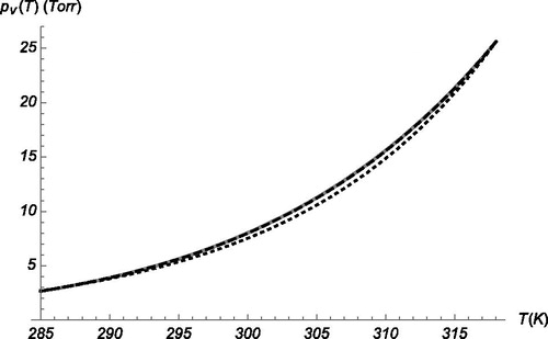
Figure 2 includes also the quadratic exponent n(T)=n_sexp[a₁(T−T_s)+a₂(T−T_s)²] (black dashed; obtained by fitting a quadratic curve to the ln(n_eq) vs. T data), indistinguishable from the vapor pressure data (continuous gray).

We next define the dimensionless concentration N and the new dimensionless x and y variables: (14a-d) $$N=n/n_{eq}\left(T_s\right);\mathrm{ }z=x{T}_o\beta /T_s{}^2;\mathrm{ }{z}_o=\Delta T_o\beta /T_s{}^2;\mathrm{ }{Y}_D{}^3=y^{3}a{T}_o\beta /(D{T}_s{}^2),$$(14a-d) where N is a dimensionless vapor concentration, z is a rescaled axial variable making the dimensionless form of the simplified vapor pressure expression universal (=e^−z) and Y a dimensionless y chosen such as to remove all free parameters from the diffusion Equation (2a)(2a) $$ay\partial n/\partial x=D{\partial }^{2}n/\partial y^2$$(2a) . This reduces the problem to the following parameter-free form, fully describable via a single numerical integration: (15) $$\frac{\partial N}{\partial z}=\frac{1}{Y_D}\frac{{\partial }^{2}N}{\partial {Y_D}^2}$$(15) (16) $$N=e^{-z} \text{at} Y_D=0$$(16) (17) $$N=1\mathrm{ }\text{at}\mathrm{ }\text{either} z=0 \text{or} Y_D\to \infty .$$(17)

The integration requires some care because the problem is singular at Y_D=0. For this reason we have developed an alternative method of integration short-circuiting this singularity, with the additional advantage that it allows for the use of quadratic exponential fits for the vapor pressure curve (not explicitly pursued here). The method involves separation of variables in (15(15) $$\frac{\partial N}{\partial z}=\frac{1}{Y_D}\frac{{\partial }^{2}N}{\partial {Y_D}^2}$$(15) ) though not in terms of z and Y_D, but rather in terms of z and the similarity variable η_D: (18) $$z\prime =z;{\eta }_D=Y_D/z^{1/3}=\eta L{e}^{1/3};\mathrm{ }Le=\alpha /D.$$(18)

(15(15) $$\frac{\partial N}{\partial z}=\frac{1}{Y_D}\frac{{\partial }^{2}N}{\partial {Y_D}^2}$$(15) ) then becomes (19) $$z\frac{\partial N}{\partial z}=\frac{1}{{\eta }_D}\frac{{\partial }^{2}N}{\partial {{\eta }_D}^2}+\frac{{\eta }_D}{3}\frac{\partial N}{\partial {\eta }_D},$$(19) where we have dropped the prime in z’ for notational brevity. It is convenient to define the related quantity Y such that η, defined in (6), may be written as Y/z^1/3, such that Y_D/Y = η_D/η = Le^1/3. (19(19) $$z\frac{\partial N}{\partial z}=\frac{1}{{\eta }_D}\frac{{\partial }^{2}N}{\partial {{\eta }_D}^2}+\frac{{\eta }_D}{3}\frac{\partial N}{\partial {\eta }_D},$$(19) ) is separable and admits solutions of the form (20) $$N(z,{\eta }_D)=z^k{F}_k({\eta }_D),$$(20) where the F_k functions satisfy: (21) $$F_k″({\eta }_D)+{\eta }_D{}^2{F}_k\prime ({\eta }_D)/3-k{\eta }_D{F}_k({\eta }_D)=0.$$(21)

The eigenvalues k may be fixed in a variety of ways depending on the boundary conditions. In the present case, since the boundary conditions for T and n at Y = 0 are given as analytical functions of z (i.e., βz or e^−z), they can only be represented in terms of other analytic functions. Because the functions z^k are only analytic when k is a positive integer, the eigenvalues k must be positive integers. The appropriate expansion of the boundary condition in terms of these eigenfunctions is then just a Taylor series in powers of z. If the insulator was shaped as a pair of opposed wedges meeting at their vertices to minimize heat transfer, Laplace’s equation for purely conductive heat transfer in polar coordinates (r, θ) would have solutions of the form r^k(A sinkθ +B sinkθ). The wall temperature would then be of the form r^k, with non-integer values of k. In the region downstream from the insulator we will see that the eigenvalues would be negative integers. In the special case k = 0 the downstream solution has no x dependence (other than through η and η_D). This corresponds to a fixed downstream wall temperature, which applies to the problem with an abrupt jump between two fixed wall temperatures (Fernandez de la Mora 2020). The function F₀(η) will therefore play a leading role in describing the temperature and vapor concentration past the insulator. The case k = 1 applies to the constant wall temperature gradient problem previously analyzed. The solutions to (15–17) may be constructed by expanding in powers of z both the exponential boundary condition and the solution N(z,η_D): (22) $$e^{-z}=1+\sum _{k=1}^{\mathrm{\infty }}\frac{{(-z)}^k}{k!}$$(22) (23) $$N\left(z,{\eta }_D\right)=1+\sum _{k=1}^{\mathrm{\infty }}\frac{F_k\left({\eta }_D\right)}{k!}{(-z)}^k.$$(23)

The following boundary conditions apply to the F_k functions: (24a,b) $$F_k\left(0\right)=1;\mathrm{ }{F}_k(\infty )=0.$$(24a,b) (21–24) has simple solutions involving polynomials and the functions exp(−η³/9) and Γ(1/3,−η³/9) previously encountered in (9(9) $$F_1\left(\eta \right)=\frac{\left(6+{\eta }^3\right)\mathrm{\Gamma }\left[1/3,{\eta }^3/9\right]-3^{4/3}\mathrm{ }\eta e^{-{\eta }^3/9}\mathrm{ }}{6\Gamma (1/3)},$$(9) ) for the description of the temperature field: (25) $$F_k\left({\eta }_D\right)=\frac{A_k\left({\eta }_D\right)\mathrm{\Gamma }\left[1/3,{\mathrm{ }{\eta }_D}^3/9\right]-{\mathrm{ }{B}_k\left({\eta }_D\right)\mathrm{ }3}^{-2/3}{\eta }_D\mathrm{ }exp(-{\mathrm{ }{\eta }_D}^3/9)}{\mathrm{\Gamma }(1/3)}.$$(25)

We have determined the first ten F_k functions by solving the corresponding differential Equation (21)(21) $$F_k″({\eta }_D)+{\eta }_D{}^2{F}_k\prime ({\eta }_D)/3-k{\eta }_D{F}_k({\eta }_D)=0.$$(21) with k from 1 to 10 via the computer program Mathematica (Figure 1). The general solution to (21(21) $$F_k″({\eta }_D)+{\eta }_D{}^2{F}_k\prime ({\eta }_D)/3-k{\eta }_D{F}_k({\eta }_D)=0.$$(21) ) involves two independent functions. One is a pure polynomial, unsuitable for our purposes here because it diverges as η→∞. The other has the structure (25), decays exponentially to zero as η increases (automatically satisfying (24b(24a,b) $$F_k\left(0\right)=1;\mathrm{ }{F}_k(\infty )=0.$$(24a,b) )) and is normalized to also satisfy (24a(24a,b) $$F_k\left(0\right)=1;\mathrm{ }{F}_k(\infty )=0.$$(24a,b) ). The first ten A_k, B_k polynomials including this normalization are collected in Table A1 in the appendix. The awkwardly large numbers in Table A1 have been expressed more economically by Stolzenburg (2020). Stolzenburg’s formulae have the advantage of extending to arbitrary values of k, and should be particularly useful to readers having no access to or familiarity with Mathematica. The online supplementary information includes a Mathematica file where the first 10 eigenfunctions are listed, and any subsequent eigenvalue may be simply determined by interested readers. The expansion (22(22) $$e^{-z}=1+\sum _{k=1}^{\mathrm{\infty }}\frac{{(-z)}^k}{k!}$$(22) ) with k up to 10 represents e^−z with an error below 1% for 0 ≤ z ≤ 2.6. Since e^2.6=13.5, this corresponds to a reduction by a factor of 13.5 in the vapor pressure from the initial to the final temperature. This range could be extended by adding terms beyond the 10th. It is nonetheless ample enough for present purposes, given that the vapor pressure of butanol changes by a factor of 9.65 in the temperature interval from 12 to 45 °C (13.3 factor from 8 to 45 °C).

Table A1. $F_k\left(x\right)={[A}_k\left(x\right)\mathrm{\Gamma }\left[1/3,x^3/9\right]-x{B}_k(x)\mathrm{ }exp(-\frac{x^3}{9})3^{-2/3}]/\mathrm{\Gamma }[1/3].$

k	Ak(x)	Bk(x)
0	1	0
1	$1+x^3/6$	$3/2$
2	$1+\left(30x^3+x^6\right)/90$	$(24+x^3)/10$
3	$1+(1080x^3+72x^6+x^9)/2160$	$(738+66x^3+x^6)/240$
4	$1+(47520x^3+4752x^6+132x^9+x^{12})/71280$	$(28728+4050x^3+126x^6+x^9)/7920$
5	$1+\frac{2494800x^3+332640x^6+13860x^9+210x^{12}+x^{15}}{2993760}$	$\frac{1364040+266220x^3+12690x^6+204x^9+x^{12}}{332640 }$
6	$1+\frac{152681760x^3+25446960x^6+1413720x^9+32130x^{12}+306x^{15}+x^{18}}{152681760}$	$\frac{76651920+19266660x^3+1246320x^6+30384x^9+300x^{12}+x^{15}}{16964640 }$
7	$1+\frac{1}{9160905600}(10687723200x^3+2137544640x^6+148440600x^9+4498200x^{12}+64260x^{15}+420x^{18}+x^{21})$	$\frac{4981752720+1539881280x^3+126398880x^6+4148280x^9+61830x^{12}+414x^{15}+x^{18}}{1017878400 }$
8	$1+\frac{1}{632102486400}(842803315200x^3+196654106880x^6+16387842240x^9+620751600x^{12}+11823840x^{15}+115920x^{18}+552x^{21}+x^{24})$	$\frac{1}{70233609600 }(367847101440+135418106880x^3+13513443840x^6+559120320x^9+11175840x^{12}+112698x^{15}+546x^{18}+x^{21})$
9	$1+\frac{1}{49303993939200}(73955990908800x^3+19721597575680x^6+1917377542080x^9+87153524640x^{12}+2075083920x^{15}+27125280x^{18}+193752x^{21}+702x^{24}+x^{27})$	$\frac{1}{5478221548800 }(30427717703040+13030432934400x^3+153448047040x^6+76772836800x^9+1928324880x^{12}+26023788x^{15}+189630x^{18}+696x^{21}+x^{24})$
10	$1+\frac{1}{4289447472710400}(7149079121184000x^3+2144723736355200x^6+238302637372800x^9+12637261072800x^{12}+361064602080x^{15}+5899748400x^{18}+56188080x^{21}+305370x^{24}+870x^{27}+x^{30})$	$\frac{1}{476605274745600}(2787798587212800+1363968851414400x^3+185445982656000x^6+10899799447680x^9+330122459520x^{12}+5588295300x^{15}+54432000x^{18}+300240x^{21}+864x^{24}+x^{27})$

Note: Polynomials A_k(x) and B_k(x) may also be obtained for arbitrary k by explicit formulae for A_k(x) or recurrence relations for B_k(x) (Stolzenburg 2020). A Mathematica program for computing these eigenfunctions is included in the supplementary information.

2.1. Generalization to arbitrary p_v(T) and T(z) forms

Note that the particular form of the vapor pressure curve only enters into the picture through the boundary condition for the N field. While the real ln(p_v) curve of most substances is not linear with T over a wide T range, a quadratic fit is excellent even beyond the 12–45 °C range considered here. Since T at the wall is linear in x, this means that the wall boundary condition for N is well approximated by the exponential of a second order polynomial in x, which in terms of z would have the form N(z,0)=exp(−z + cz²). Note that any vapor pressure may be expanded in a Taylor series irrespective of whether it approaches the Clausius-Clapeyron form. exp(−z + cz²) may be expanded in a Taylor series very much as e^-z, though the expansion coefficients would depend on the quadratic parameter c rather than having the universal (parameter-independent) form (22(22) $$e^{-z}=1+\sum _{k=1}^{\mathrm{\infty }}\frac{{(-z)}^k}{k!}$$(22) ). For example, a quadratic fit of the vapor pressure data would yield the values of the a₁, a₂ constants in the general expression n_eq(T)=n_sexp[a₁(T−T_s)+a₂(T−T_s)²], while T−T_s at the wall is given by (5(5) $$T=T_s-x\beta F_1(\eta )\mathrm{ }\text{for}\mathrm{ }0<x<\Delta$$(5) ) as −βx, resulting in the boundary condition N(z,0)=exp[−a₁βx + a₂β²x²]. One would then choose z = a₁βx and infer the value of the coefficient c = a₂/a₁². The solution for N would then have the same structure as (23(23) $$N\left(z,{\eta }_D\right)=1+\sum _{k=1}^{\mathrm{\infty }}\frac{F_k\left({\eta }_D\right)}{k!}{(-z)}^k.$$(23) ), though with c-dependent coefficients. The quantity c is naturally specific for each condensing fluid in a given relatively broad temperature range. Therefore, the method used here to deal with the constant temperature gradient wall is extendable to most real fluids.

Another possible generalization is that the wall temperature T(z) in the insulator does not need to be strictly linear in z, as long as it may be expanded in a Taylor series.

2.2. Saturation ratio field in the constant wall temperature gradient region

In view of the description just given for n and T, we may write the saturation ratio as (26) $$S=e^{z{F}_1\left(\eta \right)}[1+\sum _{k=1}^{\mathrm{\infty }}\frac{F_k\left(\eta {Le}^{1/3}\right)}{k!}{(-z)}^k],$$(26) where an expansion keeping up to 10 F_k term is accurate for 0 ≤ z ≤ 2.6. 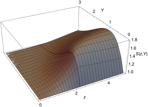Note that the details of the vapor pressure curve are absorbed in the definition of the quantity z, so the only parameter (other than the coordinates z, η) entering into (26(26) $$S=e^{z{F}_1\left(\eta \right)}[1+\sum _{k=1}^{\mathrm{\infty }}\frac{F_k\left(\eta {Le}^{1/3}\right)}{k!}{(-z)}^k],$$(26) ) is the diffusivity ratio Le. The S(z,Y) surface shown in Figure 3 is for Le = 1. The general form of S(z,Y) is similar for Le = 2.5, though with higher S_max. One can see that for various wall distances Y (fixed streamlines), S increases monotonically with z up to the end of the insulator region. Determination of the maximum saturation ratio achieved along each streamline therefore requires continuing the description of the problem into the constant wall temperature region. Note however that the implicit identification made here between the point of maximal saturation ratio and the point where the nucleation rate is dominating is not exact when the physical properties of the gas/vapor system (temperature, surface tension γ and molecular volume v_o) are position-dependent. In general the nucleation rate is a function of S as well as these physical properties. This dependence is different for different nucleation models, and cannot be given in general. For the classical (capillary) model of nucleation on charged particles the main governing parameter is the quantity ${\alpha }_S=\sqrt{\frac{q^2(1-1/ϵ)}{64{\pi }^2{ϵ}_o\gamma }3}\frac{k_{B}T}{2\gamma v_o}lnS,$ where q is the charge on the particle, ε is the dielectric constant of the condensed vapor, k_B is Boltzmann’s constant (Seto et al. 1997). For large enough particles (charged or neutral) the appropriate parameter is the Kelvin diameter (Stolzenburg and McMurry 1991). The variable S and its maximum value are therefore chosen here to provide an approximate indication rather than an exact description of where the nucleation rate is maximized.

Figure 3. Saturation ratio (26) versus dimensionless variables z, Y for an exponential vapor pressure and Le = 1. The insulator region corresponds to z < z_o=2.264. The early part of the constant wall temperature region (z_o < z < 5) is also included. As one moves along the ridge, at small Y (and z) S_max is close to unity. At larger Y (or z) the top of the ridge becomes flat, resulting in a constant asymptote for S_max(Y). Recall that z=z_o(x/Δ).

2.3. Saturation ratio field in the constant wall temperature region

At the value of z = z_o where the wall boundary condition changes from a fixed gradient to a constant temperature T_c and vapor concentration n_c=n_eq(T_c), the initial conditions for n(y) and T(y) are known from the calculations in the previous section. The special feature that the downstream region does not affect the upstream behavior is a result of the parabolization of the originally elliptic problem, and is only an approximation. To continue the solution rigorously would require solving (2a,b) subject to these initial and boundary conditions: (2a) $$ay\partial n/\partial x=D{\partial }^{2}n/\partial y^2$$(2a) (2b) $$ay\partial T/\partial x=a{\partial }^{2}T/\partial y^2,$$(2b) (27) $$n\left(z,0\right)=n_c;n(z,\infty )=n_s$$(27) (28) $$T\left(z,0\right)=T_c;T(z,\infty )=T_s$$(28) (29) $$T(z_o,\eta )=T_s[1-F_1(\eta )\Delta \beta /T_s]$$(29) (30) $${n(z}_o,\eta )=n_s[1+\sum _{k=1}^{\mathrm{\infty }}\frac{F_k\left(\eta {Le}^{1/3}\right)}{k!}{(-z_o)}^k]$$(30)

Note that the expression (29(29) $$T(z_o,\eta )=T_s[1-F_1(\eta )\Delta \beta /T_s]$$(29) ) for the temperature does not involve z_o as the natural variable, but rather z_oT_s/T_o. This is the consequence of having chosen the variable z such as to simplify the expression for the equilibrium vapor pressure at Y = 0. Selecting for our calculation T_c=12 °C; T_s=45 °C, and fitting p_v(T) to a simple exponential such that the vapor pressure is correct at both extreme temperatures we find T_o/T_s=21.64. The condition that the wall temperature be 12 °C at z = z_o then fixes $$z_o=2.264,$$

and the initial condition for the temperature may be written $$[T(z_o,\eta )-T_s]/\left(T_c-T_s\right)=F_1(\eta ).$$

If this initial condition were zero rather than F₁(η), the problem would be that arising in the ideal case of a step temperature change, whose solution is strictly a function of η (Fernandez de la Mora 2020): (31) $$T-T_s=\left(T_c-T_s\right)F_0(\eta );F_0\left(\eta \right)=\frac{\mathrm{\Gamma }[1/3,\mathrm{ }{\eta }^3/9]}{\mathrm{\Gamma }[1/3]}.$$(31)

Therefore F₀(η) and F₀(ηLe^1/3) obey exactly the differential equations for (T−T_s)/(T_c−T_s) and (n−n_s)/(n_c−n_s), also meeting their boundary conditions at y = 0 and y→∞. Unfortunately F0(η) and F₀(ηLe^1/3) do not satisfy the required initial conditions. The standard procedure to satisfy them is to identify a set of eigenfunctions and represent the initial condition as a linear combination of them. A suitable set would be the same F_k functions already used, though with negative eigenvalues k such that the solution would asymptotically decay into F₀ at large z. This approach is viable because the F_-k functions satisfying F_−k(0)=F_−k(∞)=0 are readily found of the form η C_k(η)exp(−η³/9), where C_k(η) is a polynomial of order k−1 in η³. Proceeding to a sufficiently large order in k one would hope to obtain an arbitrarily accurate solution. A far less laborious though perhaps less precise calculation will be followed here based on an accurate approximation of the initial conditions in terms of the function F₀(η). The basis for this simplification is first that the initial conditions at z_o for the concentration and temperature variables both have a form combining the curves in Figure 1, with approximately exponentially decaying functions evolving from unity at the wall to zero at large enough η. This structure is given by F₀(η) for the step problem, by F₁(η) for the initial temperature profile, and by a combination of the various F_k(η_D) for the initial concentration profile. Although the widths of these various functions vary and their overall shapes are not identical, one may approximately match the two initial value functions to F₀(λs) with the factor λ suitably chosen. An even better fit to the initial conditions (with errors smaller than 0.2%; see Figure 4) can be obtained by a linear combination of two F₀(λs) functions of the form (32) $$F_1(z_o,s)\mathrm{ }\text{or}\mathrm{ }[N(z_o,s)-1]/[N_c-1]\sim \frac{F_0\left({\lambda }_{1}s\right)+b{F}_0\left({\lambda }_{2}s\right)}{1+b},$$(32) where s stands for η in the case of F₁, and for η_D in the case of [N(z_o,s)−1]. The optimal fit parameters to both initial conditions are given in Table 1. Note that the initial condition, and therefore the fit are independent of Le, since only η or η_D enter as variables in either of the two problems. The initial condition for the temperature is expressed in terms of F₁ only, so the fit obtained for F₁ is universal irrespective of the value of z_o. The initial condition for N depends on z_o, and has been computed here only for the special case z_o=2.26408 considered.

Figure 4. Comparison of the calculated initial conditions at z=z_o for the vapor concentration (top) and the temperature (bottom) with the linear combination (32) of two F₀(λs) functions (dashed). s is a generic variable for either η or η_D.

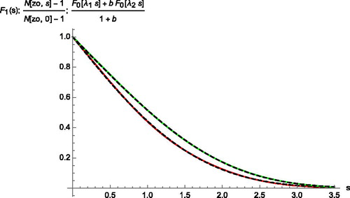
Table 1. Optimal parameters to fit the initial value functions (first column) according to (32).

	b	λ1	λ2
[T(zo,η)-Ts)/(Tc-Ts)	3.15916	2.35353	1.17383
[N(zo, ηD)-1)/[Nc-1]	5.43733	1.91207	1.09323

The legitimacy of introducing the factors λ_i while preserving the validity of the solution to the constant wall temperature problem requires some elaboration. In reality F₀(λη) is not a solution to the governing equation for F₀(η): F₀″(η)+η²F₀′(η)/3 = 0. But the original governing equations for T and n are invariant under translations in the axial variable z, and therefore admit solutions linear in F₀[Y/(z−z₁)^1/3] or F₀[YLe^1/3/(z−z₁)^1/3], with arbitrary values of the translation constant z₁. The necessary factor λ may accordingly be introduced by shifting the virtual origin of the temperature step such that z_o-z₁=z_o/λ³, or (33) $$z_1=z_o(1-{\lambda }^{-3}).$$(33)

An exact solution to the constant wall temperature problem is accordingly $F_0\left[\frac{Y}{{(z-z_o+z_o{/{\lambda }_1}^3)}^{1/3}}\right].$ The desired combinations of two such exact solutions matching with excellent approximation (Figure 4) the initial conditions are accordingly: (34a) $$[T(z,Y)-T_s)/(T_c-T_s)\approx F_T(z,Y)=\frac{F_0[\frac{Y}{{(z-z_o+z_o/{2.35353}^3)}^{1/3}}]+3.15916F_0[\frac{Y}{{(z-z_o+z_o/{1.17383}^3)}^{1/3}}]}{4.15916}$$(34a) (34b) $$[n(z,Y)-\mathrm{ }{n}_s)/[n_c-\mathrm{ }{n}_s]\approx \mathrm{ }{F}_N(z,Y)=\frac{F_0[\frac{YL{e}^{1/3}}{{(z-z_o+z_o/{1.91207}^3)}^{1/3}}]+5.43733F_0[\frac{YL{e}^{1/3}}{{(z-z_o+z_o/{1.09323}^3)}^{1/3}}]}{6.43733}$$(34b)

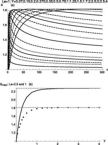
These are the approximate solutions to the problem we shall use in the constant wall temperature region z > z_o. The corresponding saturation ratio may be written as: (35) $$S\left(z,Y\right)=\left[1+(\hspace{0.17em}\text{exp}\hspace{0.17em}\right[-z_o\left]-1)F_N\left(z,Y\right)\right]\hspace{0.17em}\text{exp}\left[z_o{F}_T\left(z,Y\right)\right],$$(35) with F_N(z,Y) and F_N(z,Y) defined in (34a,b). This S(z,Y) prediction is displayed in Figure 3 for Le = 1 for moderately small values of z ≥ z_o, showing a good match at z = z_o with the solution previously obtained for z ≤ z_o. Figure 5a shows saturation ratio profiles S(z) at substantially larger z values, each curve calculated for a different fluid streamline with fixed Y. The slope is discontinuous at z = z_o, most markedly for the smaller Y values, as may be more clearly seen in Figure 3. For Y = 0.07 the maximum of S arises at z = z_o, while at Y ≥ 0.15 it arises further downstream. The maximal saturation ratio achieved along each of these streamlines is shown in Figure 5b as a function of the corresponding Y value for Le = 1 (bottom data points) and 2.5 (top continuous curve). One can see that a constant S_max(Y) asymptote is quickly reached at values of Y modestly above unity. Therefore, the effect of the finite extent of the insulator strip is limited to a boundary layer (BL) near the wall, where S values between unity and the asymptotic value are encountered. The dependence of the thickness of this boundary layer on Le is imperceptible in the range 1 < Le < 2.5 considered. As long as this region is thin, the fraction of the particles contained in it will be small, hardly affecting the overall response of the CPC. In cases when this region is not so narrow, its effects can be removed by using sheath gas. Near-wall sheath gas brings in an extra practical benefit, as the level of particle activation along a streamline depends not only on S_max (entering in the exponent of the nucleation rate) but is additionally linear in the residence time in the close vicinity of the point of maximal nucleation rate. This linear effect is generally minor compared with the effect of the changes in the exponent, except near the wall, where this residence time tends to zero (Fernandez de la Mora 2020). Most of the resulting streamline dependence of the activation level remaining even when S_max is uniform is accordingly effectively removed by the sheath gas.

Figure 5. (a) Calculated axial variation of the saturation ratio S(z) for Le = 1 at various wall distances Y (indicated in the legend by its right asymptote, from bottom to top). (b) S_max versus Y for Le = 1 (bottom points, taken as the maxima for each Y value in (a)) and Le = 2.5 (top curve). Notice the minimal dependence of the boundary layer thickness on Le.

Worthy of note is the fact that the asymptotic S_max obtained outside the boundary layer (2.285 for Le = 2.5) matches almost exactly the value obtained for a discontinuous temperature jump (2.287), for which S takes the form (36) $$S_{\infty }\left(z,Y\right)=\left[1+(\hspace{0.17em}\text{exp}\hspace{0.17em}\right[-z_o\left]-1)F_0\right[Y{\left(Le/z\right)}^{1/3})\left]\hspace{0.17em}\text{exp}\hspace{0.17em}\right[z_o{F}_0\left(Y/z^{1/3}\right)].$$(36)

The slight difference found in the fourth significant figure for S_max is to be expected given the approximate nature of the initial condition used at z_o. Accordingly, one may safely conjecture that the solution with a finite insulating strip tends exponentially fast into the ideal solution without insulator.

2.4. Boundary layer thickness

The problem has been analyzed in terms of the variables z, Y, convenient to describe the exponential vapor pressure. To quantify the boundary layer (BL) thickness it is preferable to use the natural variables for the diffusive problem. z_o is defined from p_v(T_s)/p_v(T_c)=exp(z_o), which based on the actual ratio of vapor pressures for butanol at 12 and 45 °C gives z_o=2.264. In our model for the vapor pressure, N_eq(T)=exp[T_o(T−T_s)/T_s²], which particularized at T = T_c gives z_o=T_o(T_s−T_c)/T_s². Accordingly z = xT_oβ/T_s²=T_o(T_s−T_c)/T_s² x/Δ = z_ox/Δ. Similarly Y³ = y³aT_o(T_s−T_c)/(ΔαT_s²)= y³az_o/(Δα). Hence (37a) $$z=z_{o}x/\Delta$$(37a) (37b) $$Y=y{[a{z}_o/(\Delta \alpha )]}^{1/3}.$$(37b)

Therefore, since the BL thickness found in Figure 5 corresponds to Y∼1, for a planar channel of half-width R the BL width Δy is (38) $$\Delta y/R={[(\Delta \alpha )/\left(R^{3}a{z}_o\right)]}^{1/3}.$$(38)

For planar Poiseuille flow, the velocity field is u=(3/2)U_o[1−(R−y)²/R²)], where U_o is the mean velocity. In this case [du/dy]_y=0=a = 3U_o/R, resulting in (39) $$\Delta y/R={[(\Delta \alpha )/\left(3R^2{U}_o{z}_o\right)]}^{1/3}.$$(39)

Adopting as an example dimensions similar to those of Kanomax’s rectangular fast CPC, we take Δ = 4mm, R = 0.5 mm, α = 0.211 cm²/s, U_o=1 m/s, resulting in Δy/R = 0.367. This BL region would be removed by using 17.7% of sheath gas, while Kanomax’s fast CPC uses 50% sheath gas. Therefore, even for an outrageously long insulator strip with Δ/R∼8 in a CPC with an unusually narrow channel width (2R = 1mm), the effect of the insulator strip may be counteracted by a modest proportion of sheath gas. Note however that the near-wall assumption (u = ay) used in this study would result in non-negligible errors when Δy/R = 0.367. If the insulating strip were reduced to 0.5 mm one would obtain Δy/R = 0.1835. Modeling the fluid velocity in this BL region by the near-wall assumption adopted here would involve a tolerable 10% error at the BL edge, and the influence of the boundary layer would be removed by using just 4.74% of sheath gas. Note however that removal of this BL does not suffice to produce uniform saturation ratio profiles everywhere in any CPC using conventional fluids such as butanol, not even with 50% sheath. This additional improvement requires the use of vapor/gas combinations having a Lewis number near unity.

3. Conclusions

We have considered the effect of an insulator strip spreading the saturator-condenser temperature change over a region of finite length Δ. The analysis presented has shown that the flow domain affected by the strip is restricted to a small BL near the wall. Notably, the perturbation from the strip decays exponentially toward the core flow, where the behavior is exactly as in the ideal case of a discontinuous temperature jump. While the BL region where S_max(ψ) decays to unity is an unavoidable consequence of an insulating strip of finite length, its effects are strictly local and can be counteracted via modest fractions of sheath gas.

These findings show that the recent proposal of Fernandez de la Mora (2020) to use DCPCs for high resolution particle sizing and basic heterogeneous nucleation studies is not irreparably impaired by the finite length of the insulator.

The analysis presented is restricted to a simple exponential model for the vapor pressure, and to a linear temperature profile over the insulator strip. However, the general conclusions drawn are far more general. This is expected because the solution method involves an expansion like (23(23) $$N\left(z,{\eta }_D\right)=1+\sum _{k=1}^{\mathrm{\infty }}\frac{F_k\left({\eta }_D\right)}{k!}{(-z)}^k.$$(23) ) with all the F_k(η) terms in the expansion decaying exponentially with η. A more general situation with arbitrary temperature profiles over the insulator wall, and arbitrary vapor pressure curves would preserve that structure, simply changing the numerical values of the coefficients, but not the BL-like exponentially fast decay observed here.

Nomenclature
a	=	velocity gradient at the wall (1(1) $$u\left(x,\mathrm{ }y\right)=ay.$$(1) )
a1, a2	=	constants in the quadratic fit of the vapor pressure curve, neq(T)= nsexp[a1(T-Ts)+a2(T-Ts)2]
c	=	a2/a12: quadratic coefficient in the representation of neq vs. z: neq(z)= nsexp[-z + cz2]
C(S)	=	saturation ratio spectrum obtained as the CPC output upon scanning over S
D	=	vapor diffusivity entering in (2a)
Fk(η)	=	eigenfunctions solving (21(21) $$F_k″({\eta }_D)+{\eta }_D{}^2{F}_k\prime ({\eta }_D)/3-k{\eta }_D{F}_k({\eta }_D)=0.$$(21) ) with boundary conditions (24), expressed as (25(25) $$F_k\left({\eta }_D\right)=\frac{A_k\left({\eta }_D\right)\mathrm{\Gamma }\left[1/3,{\mathrm{ }{\eta }_D}^3/9\right]-{\mathrm{ }{B}_k\left({\eta }_D\right)\mathrm{ }3}^{-2/3}{\eta }_D\mathrm{ }exp(-{\mathrm{ }{\eta }_D}^3/9)}{\mathrm{\Gamma }(1/3)}.$$(25) ) via Table A1
FT, FN	=	approximate expression solutions (34a-b) for constant wall temperature region z > zo
n	=	vapor number concentration (cm−3)
neq(T)=pv(T)/(kBT)	=	equilibrium number concentration of the vapor
ns	=	neq(Ts)
nc	=	neq(Tc)
N	=	n/ns
k	=	integer number Eigenvalues appearing in (20(20) $$N(z,{\eta }_D)=z^k{F}_k({\eta }_D),$$(20) ), characteristic of eigenfunctions Fk(η)
kB	=	Boltzmann’s constant
pv(T)	=	equilibrium vapor pressure for working fluid
q	=	charge on the particle
R	=	half height of channel
S = n/neq(T)	=	saturation ratio
Smax(Y)	=	maximal saturation ratio along a fixed fluid streamline at constant Y
S∞	=	maximal saturation ratio in the solution for the sudden temperature jump problem (Δ = 0 limit) for which S is given in (36). We conjecture that S∞= Smax(∞).
T	=	absolute temperature
To	=	activation temperature in Clasius-Clapeyron equation, equal to the activation energy over kB.
Ts	=	uniform wall temperature prevailing upstream of the insulator
Tc	=	uniform wall temperature prevailing downstream of the insulator
Uo	=	characteristic velocity in fully developed plane Poiseuille flow, given from a=3Uo/R
u(x,y)	=	axial velocity field, approximated as (1(1) $$u\left(x,\mathrm{ }y\right)=ay.$$(1) ) near the wall
vo	=	molecular volume for the condensing vapor
x	=	axial coordinate along the flow direction
y	=	Cartesian coordinate normal to the wall, vanishing at the wall
Y	=	z1/3η: dimensionless y defined following (19(19) $$z\frac{\partial N}{\partial z}=\frac{1}{{\eta }_D}\frac{{\partial }^{2}N}{\partial {{\eta }_D}^2}+\frac{{\eta }_D}{3}\frac{\partial N}{\partial {\eta }_D},$$(19) )
YD	=	z1/3ηD: dimensionless y defined in (14d)
z	=	dimensionless axial coordinate in model vapor pressure curve neq(T)=nsexp[a1(T-Ts)], chosen such that the wall vapor concentration can be simply written as nse-z
zo	=	value of z at x = Δ.
z1	=	virtual origin of axial variable z (33), optimally fitting the initial conditions (32b-c) for the problem downstream the insulator
α	=	thermal diffusivity appearing in (2b(2b) $$ay\partial T/\partial x=\alpha {\partial }^{2}T/\partial y^2,$$(2b) )
${\alpha }_S=\sqrt[3]{\frac{q^2(1-1/ϵ)}{64{\pi }^2{ϵ}_o\gamma }}\frac{k_{B}T}{2\gamma v_o}lnS$	=	activation parameter for ions in capillary (Kelvin-Thomson) theory
β	=	minus the temperature gradient in the insulator (3a(3b) $$\text{for}\mathrm{ }x=0,T=T_s\mathrm{ }\text{for}\mathrm{ }\text{all}\mathrm{ }y>0.$$(3b) )
Δ	=	axial length of the thermal insulator (3a(3a) $$T=T_s\mathrm{ }\text{for}\mathrm{ }x<0,\mathrm{ }\text{and}\mathrm{ }T=T_s-\beta x\mathrm{ }\text{for}\mathrm{ }0<x<\Delta \mathrm{ }\text{and}\mathrm{ }y=0,$$(3a) )
ε	=	dielectric constant of condensed vapor
εo	=	electrical permittivity of vacuum
ψ	=	stream function, constant at constant y in fully developed flow
η	=	similarity variable defined in (6(6) $$\eta =y{a}^{1/3}/{(\alpha x)}^{1/3}.$$(6) )
ηD=ηLe1/3	=	defined in (18b(18) $$z\prime =z;{\eta }_D=Y_D/z^{1/3}=\eta L{e}^{1/3};\mathrm{ }Le=\alpha /D.$$(18) )
γ	=	surface tension of condensed vapor
λ1, λ2	=	scaling factors used to approximately describe the initial conditions at x=Δ in (32), with numerical values given in Table 1

Acknowledgments

I am grateful to Dr. Derek Oberreit and Steve Kosier from Kanomax for encouraging the present studies through the loan of Kanomax’s fast CPC, and through invaluable discussions on its characteristics. My interest in laminar diffusive CPCs owes much to many conversations with Professor Michel Attoui.

Additional information

Funding

Partial support from NIH SBIR Phase I Grant Number 1 R43 GM131542-01A1 (National Institute of General Medical Sciences, under Dr. Dmitriy Krepki) is gratefully acknowledged.

Appendix A:

Polynomials A_k, B_k defining the eigenfunctions F_k(x)

References

- Agarwal, J. K., and G. J. Sem. 1980. Continuous flow, single-particle-counting condensation nucleus counter. J. Aerosol Sci. 11 (4):343–57. doi:10.1016/0021-8502(80)90042-7.
- Kangasluoma, J., A. Franchin, J. Duplissy, L. Ahonen, F. Korhonen, M. Attoui, J. Mikkilä, K. Lehtipalo, J. Vanhanen, M. Kulmala, et al. 2016. Operation of the Airmodus A11 nano Condensation Nucleus Counter at various inlet pressures and various operation temperatures, and design of a new inlet system. Atmos. Meas. Tech. 9 (7):2977–88. doi:10.5194/amt-9-2977-2016.
- Fernandez de la Mora, J. 2020. Viability of basic heterogeneous nucleation studies with thermally diffusive condensation particle counters. J. Coll. Int. Sci. in press.
- Fernandez de la Mora, J. 2011. Heterogeneous nucleation with finite activation energy and perfect wetting: Capillary theory versus experiments with nanometer particles, and extrapolations on the smallest detectable nucleus. Aerosol Sci. Technol. 45 (4):543–54. doi:10.1080/02786826.2010.550341.
- Gamero-Castaño, M., and J. Fernandez de la Mora. 2000. A Condensation Nucleus Counter (CNC) sensitive to singly charged subnanometer particles. J. Aerosol Sci. 31 (7):757–72. doi:10.1016/S0021-8502(99)00555-8.
- Hering, S. V., M. R. Stolzenburg, F. R. Quant, D. R. Oberreit, and P. B. Keady. 2005. A laminar-flow, water-based condensation particle counter (WCPC), Aerosol Sci. Technol. 39 (7):659–72. doi:10.1080/02786820500182123.
- Kogan, J. I., and A. G. Burnasheva. 1960. Growth and measurement of condensation nuclei in a continuous stream. Phys. Chem. Moscow 34:2630.
- Lewis, G. S., and S. V. Hering. 2013. Minimizing concentration effects in water-based, laminar-flow condensation particle counters . Aerosol Sci. Technol. 47 (6):645–54. doi:10.1080/02786826.2013.779629.
- Liñán, A. 1974. The asymptotic structure of counterflow diffusion flames for large activation energies. Acta Astronaut. (UK) 1 (7-8):1007–39. doi:10.1016/0094-5765(74)90066-6.
- Marti, J. J., R. J. Weber, M. T. Saros, J. G. Vasiliou, and P. H. McMurry. 1996. Modification of the TSI 3025 condensation particle counter for pulse height analysis. Aerosol Sci. Technol. 25 (2):214–8. doi:10.1080/02786829608965392.
- Okuyama, K., Y. Kousaka, and T. Motouchi. 1984. Condensational growth of ultrafine aerosol-particles in a new particle-size magnifier. Aerosol Sci. Technol. 3 (4):353–66. doi:10.1080/02786828408959024.
- Oberreit, D. 2017. Compact condensation particle counter technology, US Patent. Application 20170276589.
- Reischl, G. P., J. M. Makela, R. Karch, and J. Necid. 1996. Bipolar charging of ultrafine particles in the size range below 10 nm. J. Aerosol Sci. 27 (6):931–49. doi:10.1016/0021-8502(96)00026-2.
- Saros, M. T., R. J. Weber, J. J. Marti, and P. H. McMurry. 1996. Ultrafine aerosol measurement using a condensation nucleus counter with pulse height analysis. Aerosol Sci. Technol. 25 (2):200–13. doi:10.1080/02786829608965391.
- Seto, T., K. Okuyama, L. de Juan, and J. Fernández de la Mora. 1997. Condensation of supersaturated vapors on monovalent and divalent ions of varying size. J. Chem. Phys. 107 (5):1576–85. doi:10.1063/1.474510.
- Stolzenburg, M. R. 2020. Comments on “Effect of the finite width of the temperature transition in diffusive condensation particle counters” by J. Fernandez de la Mora, Aerosol Sci. Tech., this issue.
- Stolzenburg, M. R., and P. H. McMurry. 1991. An Ultrafine AerosolCondensation Nucleus Counter. Aerosol Sci. Technol. 14 (1):48–65. doi:10.1080/02786829108959470.
- Tauber, C., X. Chen, P. E. Wagner, P. M. Winkler, C. J. Hogan, Jr., and A. Maißer. 2018. Heterogeneous nucleation onto monoatomic ions: Support for the Kelvin-Thomson Theory. Chemphyschem 19 (22):3144–9. doi:10.1002/cphc.201800698.
- Vanhanen, J., J. Mikkila, K. Lehtipalo, M. Sipila, H. E. Manninen, E. Siivola, T. Petaja, and M. Kulmala. 2011. ParticleSize magnifier for Nano-CN detection. Aerosol Sci. Technol 45 (4):533–42. doi:10.1080/02786826.2010.547889.
- Wilson, C. T. R. 1927. On the cloud method of making visible ions and the tracks of ionizing particles. In Nobel lectures: Physics. New York: Elsevier.
- Winkler, P. M., G. Steiner, A. Vrtala, H. Vehkamäki, M. Noppel, K. E. J. Lehtinen, G. P. Reischl, P. E. Wagner, and M. Kulmala. 2008. Heterogeneous Nucleation Experiments Bridging the Scale from Molecular Ion Clusters to Nanoparticles. Science 319 (5868):1374–7. doi:10.1126/science.1149034.