Coupling an online ion conductivity measurement with the particle-into-liquid sampler: Evaluation and modeling using laboratory and field aerosol data

Abstract

A particle-into-liquid sampler (PILS) was coupled to a flow-through conductivity cell to provide a continuous, nondestructive, online measurement in support of offline ion chromatography analysis. The conductivity measurement provides a rapid assessment of the total ion concentration augmenting slower batch-sample data from offline analysis and is developed primarily to assist airborne measurements, where fast time-response is essential. A conductivity model was developed for measured ions and excellent closure was derived for laboratory-generated aerosols (97% conductivity explained, R² > 0.99). The PILS-conductivity measurement was extensively tested throughout the NASA Cloud, Aerosol and Monsoon Processes: Philippines Experiment (CAMP²Ex) during nineteen research flights. A diverse range of ambient aerosol was sampled from biomass burning, fresh and aged urban pollution, and marine sources. Ambient aerosol did not exhibit the same degree of closure as the laboratory aerosol, with measured ions only accountable for 43% of the conductivity. The remaining fraction of the conductivity was examined in combination with ion charge balance and found to provide additional supporting information for diagnosing and modeling particle acidity. An urban plume case study was used to demonstrate the utility of the measurement for supplementing compositional data and augmenting the temporal capability of the PILS.

EDITOR:

• Jim Smith

Introduction

The particle-into-liquid sampler (PILS, Brechtel Manufacturing Inc.) is a droplet impaction device used to facilitate a selection of offline and online aerosol composition techniques (e.g., Weber et al. 2001; Sorooshian et al. 2006a; Sullivan et al. 2004; Rastogi et al. 2009; Hecobian et al. 2010; Saarnio et al. 2013; Zhang et al. 2016). Briefly, the sample airstream is mixed with steam to create a highly supersaturated environment whereby aerosol particles activate into droplets and rapidly grow. The droplets are collected by inertial impaction and continuously rinsed and transported from the impactor surface to an online analytical device or storage vials. Concentrations and properties of dissolved species in the aqueous stream can be subsequently related back to the sampled aerosol.

The performance of the PILS has been extensively tested (Weber et al. 2001; Orsini et al. 2003) and modeled (Sorooshian et al. 2006a), and the combination of the PILS with either online or offline ion chromatography (IC) has become a mainstay of its implementation for laboratory (Surratt et al., 2007; Kenseth et al. 2018; Wonaschütz et al. 2019) and field (Li et al. 2004; Lee et al. 2008; Hersey et al. 2011; Xue et al. 2014; Youn et al. 2015; Nah et al. 2018) analysis of water-soluble aerosol composition, including airborne deployment (Weber et al. 2003; Lee et al. 2003; Brock et al. 2004; Sorooshian et al. 2006b, 2007, 2008, 2015; Peltier et al. 2007; Wonaschütz et al. 2012; Hersey et al. 2013; Guo et al. 2016). Offline IC offers advantages for aircraft operation by avoidance of data loss in the event of a malfunctioning online IC system and enhancements in speciation and quantification of more species such as organic acids and amines that require longer IC sample run times, which are impractical for online airborne operation. While offline analysis also allows for a multitude of additional laboratory tests, this procedure necessitates the collection and storage of many sample vials, often exceeding one hundred per flight. Aside from challenges related to operation at reduced pressure, a further airborne requirement for improved characterization of sampled aerosol is the need for enhanced temporal resolution especially at higher aircraft speeds and when sampling heterogeneous airmasses (e.g., urban plumes) or when assessing vertical structure (e.g., Lee et al. 2003; Beyersdorf et al. 2016). The batch sampling inherent with IC places a constraint on the frequency of data, with normal airborne operation requiring several minutes to collect a sample. Other techniques for determining aerosol composition, such as mass spectrometry, can better meet the temporal demands of airborne sampling but may require interpretive analysis (e.g., of the mass spectrum) to resolve aerosol-relevant species concentrations (Allan et al. 2004). Some techniques are also limited in their capacity to provide absolute concentration (e.g., Murphy et al. 2006).

For improved time response, the PILS lends itself to online analytical techniques that do not require batch sampling and can operate continuously on low sample volumes and flow rates (e.g., 100 µL min⁻¹). Conductivity measurements are commonly used across a variety of geochemical and hydrological applications (e.g., Lewis 1980; Prieto et al. 2001; McCleskey 2011) and can serve as a proxy for total dissolved solids (Gustafson and Behrman 1939; Walton 1989), an important parameter in the analysis of water quality. Conductivity is a solution property that is tightly linked to the concentration of ions, making conductometric detection a common technique used in IC systems. Furthermore, conductivity-based techniques can be applied across a wide range of ion concentrations and electrodes can be miniaturized for applications involving small sample volumes. The technique is also conceptually nondestructive, which provides an opportunity to combine it with other analyses, such as online or offline IC.

One area where a synergistic opportunity exists is in providing independent closure with measured ion concentrations, through theory or models that relate measured ion concentrations to conductivity. Analysis of charge balance is often used in conjunction with IC analysis for (i) quality assurance, (ii) to assess the completeness of the measured ions, and (iii) to assess the degree of neutralization and infer sample pH. Extension to a quantitative proxy measurement of aerosol pH is made challenging by the high sensitivity to aerosol water content and the buffering effect of dissociation equilibria (Hennigan et al. 2015). A further justifiable criticism of ion balance noted by Hennigan et al. (2015) is the propagation of error that occurs when attempting to quantify a small residual charge difference from a larger collective ion concentration. The conductivity is particularly sensitive to H⁺ (and to a lesser extent OH^-) because of high prototropic mobility (5-7 times greater than other cations) via the Grotthuss mechanism (de Grotthuss 1806; Agmon 1995). This makes its inclusion as an independent measurement a useful addition to support or refute conclusions drawn from charge balance alone.

These attributes are particularly attractive for inclusion with the existing PILS setup, and given the aforementioned benefits, have been combined with offline IC. In this article, we describe the implementation of the PILS-conductivity measurement and provide an evaluation of its performance in laboratory and field experiments using a conductivity model.

Materials and methods

Instrument description

Flow-through conductivity cell

The two-wire micro flow-through conductivity cell comprises two platinum electrodes on opposite sides of a zero-dead volume, low-volume (approximately 2 µL), flow cell. The housing and fittings are polyether ether ketone (PEEK) for chemical resistance and conveniently offer fair temperature stability. The cell geometry is identical to that used in the Sievers 800 (Ionics, Boulder, CO) total organic carbon analyzer, which uses conductometric detection of dissolved and dissociated CO₂. Two temperature compensation measurements (2-wire Pt1000 resistance temperature detector (RTD) and a negative temperature coefficient thermistor) were incorporated in the cell housing. Signal processing was carried out using an off-the-shelf analog-to-digital board (CN0359, Analog Devices) to manage the excitation of the cell set at 10 V peak-to-peak at 301 Hz, mitigating electrolysis. Through multiple gain stages, the device is reportedly capable of detecting at least four orders of magnitude of dynamic range in conductivity. Temperature, conductivity, and board diagnostics were logged at 1 Hz.

Description of PILS interface

Two micro flow-through conductivity cells were incorporated into the PILS wash and sample flows, respectively (Figure 1). The wash flow cell continuously monitored the supply of liquid entering the PILS, while the sample cell was located downstream. Past reported PILS operation (e.g., Orsini et al. 2003; Sorooshian et al. 2006a) used a tracer (either LiF or LiBr) to quantify dilution effects in combining the activated droplets with the wash flow. Here we forego the addition of an ionic tracer in order to minimize the conductivity baseline and instead use the wash flow cell to monitor the stability of the ultrapure supply water and assess pressure and temperature effects.

Figure 1. A schematic diagram of the liquid flow path for the PILS-conductivity set up. Steam-activated droplets are depicted entering the impaction nozzle from right to left.

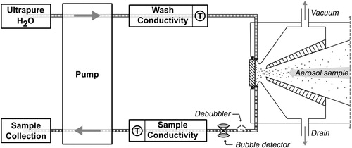
Complete details of the liquid flow path through the current PILS design are described elsewhere (Orsini et al. 2003). In summary, the wash flow is introduced at the top of an annular channel that surrounds a quartz impactor plate and the sample flow is pulled from the bottom of the channel at the lowest point. The liquid settles gravitationally around the channel, aided by a stainless steel wick. An incoming air sample containing particles is mixed with steam in the PILS chamber creating a high supersaturation environment conducive to the activation of droplets, which are accelerated through a nozzle and impacted onto the quartz impactor plate. Through the aerodynamic action of the accompanying airflow, the droplets are forced radially to the periphery of the impactor and mix with the liquid from the wash flow.

Immediately following the PILS impactor, the flow path of the current setup differs from previously documented systems (e.g., Sorooshian et al. 2006a). First, the liquid sample is passed through a vacuum bubble trap debubbler (Diba Industries), which differs in design to the “glass-Tee” debubbler described in Sorooshian et al. (2006a). This debubbler design contains an air-permeable membrane held under vacuum facilitating the removal of bubbles from the sample. At the exit of the bubble trap debubbler, a non-intrusive ultrasonic bubble detector (SMD Sensors) was attached to the sample line and used as a diagnostic, because air bubbles in the sample are problematic for the conductivity measurement. The conductivity cell is located immediately after the bubble detector and thereafter the sample is pumped to septa-capped 1 mL sample vials housed in an auto-collector (Brechtel Manufacturing Inc.) for storage and subsequent offline analyses. All connecting tubing and fittings are PEEK with 0.02 inch (0.5 mm) internal diameter, with the exception of a short length (<40 mm) of low-density polyethylene tubing required for the bubble detector. Locating the conductivity cell as close as possible to the sample output from the PILS was done to optimize time response.

The current setup is configured for aircraft operation, where fast time response is desired. PILS samples were accumulated for a duration of 150 s, which was determined as a minimum to satisfy flow rate constraints and required injection volumes for IC. The sample inlet of the PILS chamber was connected to the common aircraft inlet manifold with stainless steel tubing and the PILS was operated without an upstream impactor (e.g., PM₁) primarily to maximize the detectability of sea salt and dust constituents as well as other large particles. The phase partitioning of semi-volatile aerosol species is affected by the often large increase in sample temperature from the ambient environment (causing volatilization loss), along with the associated relative humidity decreases (causing aerosol water removal and potential liberation of solvated species). Acid and base denuders are often incorporated upstream of the PILS but are omitted here in order to (a) avoid the excess removal of gaseous species that were potentially in the particle phase at ambient conditions prior to sampling and (b) eliminate potential impaction losses for (non-volatile) large (>1 µm) particles. The adverse effect of omitting the denuders is that the data may contain contributions from soluble gases, the quantification of which requires careful consideration.

PILS-conductivity model

Conductivity is modeled as the linear sum of the individual contribution from each ionic species (x), expressed as a product of the aqueous concentration, [X] and its ionic molar conductivity, λ_x: (1) $$\kappa =\sum {\lambda }_x\left[X\right]$$(1)

The ionic molar conductivity is dependent on both temperature and concentration (Robinson and Stokes 2002, pp 126-129), resulting in a sub-linear variation of conductivity with concentration and an increase in conductivity with temperature. For each species, the ionic molar conductivity is modeled in the form: (2) $${\lambda }_x={\lambda }_{0,x}-{\mathcal{a}}_x\sqrt{\left[X\right]}$$(2) where the limiting molar conductivity, λ₀, represents the condition of infinite dilution and the factor, $\mathcal{a},$ is an empirical coefficient; both of which are generally temperature dependent. Detailed conductivity models that cover a large dynamic range (e.g., McCleskey et al. 2012a) assign species-dependent parameters for the joint concentration and temperature dependence, resulting in improved closure with measurements (McCleskey, Nordstrom, and Ryan 2012b). These models reduce to a similar form of Equation (2)(2) $${\lambda }_x={\lambda }_{0,x}-{\mathcal{a}}_x\sqrt{\left[X\right]}$$(2) at the low concentrations relevant to this application. A further simplification presumes that the temperature dependence does not vary with species, because it is predominantly driven by the solvent (water) viscosity, except in the case of H⁺ (Robinson and Stokes 2002, pp 133-143). This simplification allows the coefficients (λ₀ and $\mathcal{a}$) to be modeled as constants for each relevant ion such that the resulting conductivity is modeled at a standardized temperature. Uncorrected measurements of conductivity (κ_u) are compensated to 25 °C (by convention) using an empirical compensation factor (α): (3) $$\kappa ={\kappa }_u/\left(1+\alpha \Delta T\right)$$(3) where ΔT is the difference between the measured and standardized (25 °C) temperature. All further reported instances of measured or modeled conductivity are corrected to 25 °C, unless stated otherwise.

Strong electrolytes (e.g., KCl) dissociate fully in solution and their component ions (e.g., K⁺, Cl^-) contribute to the conductivity following Equation (1)(1) $$\kappa =\sum {\lambda }_x\left[X\right]$$(1) . The molar conductivity of the electrolyte (Λ) can be written analogous to its constituent ions (e.g., ${\mathrm{\Lambda }}_{\mathit{KCl}}={\mathrm{\Lambda }}_{0,\mathrm{ }\mathit{KCl}}-{\mathcal{A}}_{\mathit{KCl}}\sqrt{\left[\mathit{KCl}\right]}$). For a general salt containing n_x moles of x per mole of salt, (4) $${\mathrm{\Lambda }}_0=\sum {\lambda }_x{n}_x,\mathcal{ }\mathcal{A}=\sum {\mathcal{a}}_x\sqrt{n_x}$$(4)

In a mixed solution containing weak electrolytes, such as those generated by the PILS during atmospheric sampling, the concentration of certain ions may vary because of temperature dependence of dissociation equilibria. The environmental temperature in the PILS rack was not actively controlled during aircraft operation, so any large swings in environmental temperature may introduce additional sources of uncertainty beyond those expected from the simplified treatment of temperature in the conductivity model. However, to implement the model, we apply a constraining assumption that the ion concentrations at the conductivity detector remain the same through delivery into the storage vials, and until offline analysis with IC is completed. Therefore, closure analysis of the PILS-conductivity measurements with speciated ion concentrations, [X] (using IC), only requires Equations (1)-(2) and does not need further modeling of the PILS. The conductivity model coefficients (relevant to this study) are provided in Table 1.

Table 1. Ionic molar conductivity coefficients used in the conductivity model.

		λ0	$\mathcal{a}$ ^a
		(S cm^2 mol^-1)	(empirical)
Measured Cations	Na^+	50.1^b	1.83^c
	NH4^+	73.5^b	0.85^c
	K^+	73.5^b	1.49^c
	Mg^2+	106.2^b	4.26^c
	Ca^2+	119^b	6.11^c
Measured Anions	Cl^-	76.4^b	1.49^c
	NO2^-	70^d	1.9^e
	NO3^-	71.4^b	1.16^a
	SO4^2-	160^b	10.0^a
	C2O4^2-	148.5^f	12^f
Unmeasured Ions	H^+	349.9^b	2.49^a
	HCO3^-	44.1^b	0.95^a
	CO3^2-	138.8^b	7.59^a
	R^n-/n	41-66^g	–

^a Units are empirical, consistent with S cm² mol⁻¹ for a 1 mmol L⁻¹ (unit) concentration.

^b ussingestablished, theoretically derived values from ionic radii.

^c Derived using the empirical coefficients from the McCleskey (2011) model. Data are converted to the form of our simplified model by assuming T = 25 °C and 1 mmol L⁻¹ concentration (i.e., ionic strength of 1 mmol L⁻¹ for monovalent ions and 2 mmol L⁻¹ for divalent ions and assuming electroneutrality but no other ions present).

^d No available supporting experimental or theoretical data found. Estimate is based on tests with NaNO₂ using the apparatus from this study. Uncertainty is approximately 10%.

^e No available supporting data. Estimate uses the relationship between λ₀ and $\mathcal{a}$ for all other ions (except H⁺) and an interpolation using the λ₀ for NO₂^-.

^f Data reported in Bešter-Rogač et al. (2002) for Na₂C₂O₄ and K₂C₂O₄ were fit to the model used in this study to determine λ₀ and $\mathcal{a}.$ Uncertainties for λ₀ and $\mathcal{a}$ are approximately 2% and 20%, respectively.

^g Range for atmospherically relevant acids taken from data reported in Apelblat (2002).

On the other hand, relating PILS-conductivity measurements to incoming aerosol particle (and gas) mass concentrations requires such a model. This model is the same for PILS-conductivity as for relating aqueous ionic species to particulate mass and follows the mass exchange equation: (5) $$M_x{Q}_{H_{2}O}\left(\left(1+\delta \right)\left[X\right]-[{X]}_w\right)={\eta }_x{c}_x{Q}_{\mathit{AIR}}$$(5) where the left side is the net mass flux of species X in the liquid flow and the right side is the transfer of mass from the air stream to the liquid, with species dependent efficiency, η_x. Q_H2O and Q_AIR are the respective volumetric flow rate of liquid and air, δ is a dilution factor accounting for the addition of water associated with the impacted droplets, M_x is the molar mass and c_x is the mass concentration in air. [X]_w represents the aqueous concentration of X in the wash water upstream of the PILS, and the location of the wash flow conductivity cell is assumed to represent that initial state. Low-volatility, strong ionic species (e.g., SO₄^2-) are principally in the particle phase and collected with near-unit efficiency in the PILS (e.g., η_SO4 ≈ 1; Sorooshian et al. 2006a). Semi-volatile species and/or weakly dissociating ions (e.g., NH₄⁺, HCO₃^-) may have a more environmentally- and situationally dependent efficiency. In the present model, we assume that soluble, but non-dissociating species do not contribute to conductivity and suspended insoluble particles collected by the PILS (e.g., Wonaschütz et al. 2019) are ignored. Dissolved CO₂ is expected to be present in the feed water supplying the wash and representative atmospheric CO₂ mixing ratios can readily explain the 0.7-1.2 µS cm⁻¹ baseline conductivity. Operation on an aircraft at altitude results in a significant pressure differential between the cabin and inlet, and at low pressure CO₂ is liberated from solution such that [HCO₃^-] and [CO₃^2-] are reduced, making η_CO2 effectively negative. This was found to have a non-negligible impact on modeling the sample conductivity and utilizing the wash conductivity, and the appropriate incorporation of this will be discussed. The debubbler membrane is under vacuum and sensitivity tests indicate that it also can contribute to a reduction in conductivity (0.1-0.2 µS cm⁻¹), presumed to be from degassed CO₂. For the model, η_x is an umbrella for the combination of these effects. In contemporary conductivity models (e.g., McCleskey et al. 2012a) molal concentration is used by convention because it correctly accounts for temperature effects on conductivity; however, for convenience we ignore this distinction in our model because the pumping is volumetric, the solutions are dilute, and we do not seek to isolate temperature effects on volume from conductivity.

Calibration and cell performance

Calibration of the sample conductivity cell was performed using multiple dilutions of freshly prepared KCl solution standards at known concentrations ranging from 9.4 µmol L⁻¹ to 4.7 mmol L⁻¹. A background zero point was determined by measuring the conductance of the ultrapure water baseline (G₀) followed by the standards, which were stepped sequentially in concentration, before obtaining a final zero point. This procedure was conducted under relatively stable temperature conditions (29.0 ± 0.1 °C) to avoid confounding temperature effects. Operationally, the signal processing board measures the conductance (G) in the cell and relates it to conductivity, κ = K_cellG, where K_cell is the cell constant and is a user specified input based on the geometry of the conductivity cell (specifically, the ratio of the separation distance to the area of the electrodes). Throughout field operation, there was no evidence of an observed drift in the cell performance, that could be attributed to electrode fouling. During calibration, the cell constant was set to 1 cm⁻¹ and the output conductivity (or in this case, equivalently, the conductance) was compared to the known conductivity of the standard to determine the cell constant. Here we direct particular attention to characterizing the lower bound of feasible conductivity measurements, since this is near values of interest for typical ambient atmospheric conditions sampled by the PILS.

As samples become increasingly diluted, positive artifacts (e.g., sources from headspace in storage vials containing standards, and potential leaching from wetted surfaces) can make accurate calibration difficult (Spitzer et al. 2005). However, it is important for this application to understand the limiting performance at infinite dilution. A calibration curve for KCl can be constructed using: (6) $$K_{\mathit{cell}}\left(G-G_0\right)/\left[\mathit{KCl}\right]={\mathrm{\Lambda }}_{0,\mathit{KCl}}-{\mathcal{A}}_{\mathit{KCl}}\sqrt{\left[\mathit{KCl}\right]}$$(6) with a fitted intercept ${\mathrm{\Lambda }}_{0,\mathit{KCl}}$ and fitted slope $-{\mathcal{A}}_{\mathit{KCl}}.$ The ratio of the intercept of the linear fit to an established value for the limiting molar conductivity of KCl (Λ_0,KCl = 149.9 S cm² mol⁻¹) was used to derive the cell constant (K = 1.039 cm⁻¹). Repeat experiments were performed using additional strong electrolytes (NaCl, Na₂SO₄, HCl), and the fit parameters are summarized in Table 2 alongside a comparison with established data. The reported R² suggests that the measured data follows the assumed conductivity model and the limiting molar conductivity is close to expected values (within 4%), noting that for KCl it is equal, by definition, because it was the standard used to determine the cell constant. One curious behavior is the systematic underprediction of the molar conductivity at higher concentrations, reflected by the higher experimentally derived $\mathcal{A}$ coefficients compared with established data (Table 2). The systematic offset could indicate an unmodeled effect of the electronics (e.g., additional unaccounted impedance) or the electrode/cell geometry, but we cannot provide a more thorough explanation at this time. At 150 µmol L⁻¹, which is an estimated upper bound for solutions produced by PILS during laboratory tests, the difference is 8% or less depending on the electrolyte. For typical ambient aerosol concentrations, which is the primary application of this method, the difference is considerably lower (<1%), and the $\mathcal{A}$ coefficient overall becomes decreasingly important.

Table 2. Experimentally derived molar conductivity fit parameters and comparison with the conductivity model using the coefficients from Table 1.

Species	Λ0			$\mathcal{A}$
	(S cm^2 mol^-1)			(empirical units)
	Data	Model	Δ (%)	Data	Model	R^2
KCl	149.9	149.9	0^a	12.4	2.98	0.85
Na2SO4	263.9	260.2	+1.4	31.0	12.6	0.99^b
NaCl	121.9	126.5	−3.6	12.0	3.32	0.99^b
HCl	439.6	426.2	+3.1	28.3	3.98	0.97^b

^a By design, there is zero difference because KCl was used to derive the cell constant.

^b Although the correlation coefficient is high, the significance should not be interpreted further because of the low number of test points (n < 5).

Temperature compensation was performed during signal processing using the RTD data in conjunction with an empirical function relying on user defined parameters. An opportunity to calibrate the default linear temperature compensation was not possible until after most of the data was collected. Instead, the default compensation was applied and later corrected during data processing. The correction was determined using a constant 4.7 mmol L⁻¹ KCl at the standard operational flow rate, while the measured temperature of the conductivity system, PILS and other instruments was varied from 9 °C to 24 °C. The temperature correction factor (0.9% °C⁻¹) effectively incorporated the required adjustment to the temperature compensation factor and any potential offset in the RTD calibration coefficients, without needing a separate temperature reference.

Laboratory aerosol generation

Polydisperse salt aerosols were generated using a nebulizer supplied with either particle-free room air or compressed dry N₂. In either case, a fraction of the source gas bypassed the nebulizer and was used for dilution to provide rough adjustment of the aerosol concentration. The combined aerosol flow was subsequently passed through a diffusion drier to reduce the relative humidity below 40% and then was split between the PILS and a scanning mobility particle sizer (SMPS, TSI Model 3938), the latter being used to monitor the stability of the aerosol generation system and to provide an estimate of the aerosol mass concentration through integration of the mobility size distribution. Sample vials collected with the PILS were analyzed using IC (ICS-3000, ThermoFisher) for anions (Cl^-, NO₂^-, NO₃^-, SO₄^2-, C₂O₄^2-) and cations (Na⁺, NH₄⁺, K⁺, Mg²⁺, Ca²⁺) immediately upon completion of the experiment.

Ambient aerosol airborne data during the clouds, aerosols and monsoon processes, Philippines experiment (CAMP²Ex)

Nineteen airborne research flights were conducted onboard the NASA P-3 aircraft during August–October 2019 based at Clark International Airport in the Philippines. Flights targeted a diverse range of aerosol environments across the region to assess aerosol composition, optical and microphysical properties, and the complex interaction between aerosols, monsoon clouds and radiation. Noteworthy in situ sampling of distinct aerosol sources included: regionally transported smoke from biomass burning in Indonesia, local urban pollution from the Manila metropolitan area, and long-range transport of pollution from China.

Ambient aerosols were continuously sampled in flight through an isokinetic inlet (McNaughton et al. 2007) with the exception that during cloud penetrations, selected instruments were manually switched to sample from a counterflow virtual impactor inlet (CVI; Brechtel Manufacturing Inc; Shingler et al. 2012). A full description of the aerosol and trace gas payload is not provided here; rather we introduce only the instrument subset that were used to provide complementary data to support the analysis of the PILS-conductivity data. Dried (RH < 35%) and humidified (RH = 80%) total scattering were measured using two integrating nephelometers (TSI Model 3563) and particle size distributions were measured using a Laser Aerosol Spectrometer (LAS; TSI Model 3340, 100–3000 nm) with the sample flow actively dried using a Nafion dehumidifier. Non-refractory aerosol mass concentrations (<1 µm) were measured using a high-resolution time-of-flight Aerosol Mass Spectrometer (AMS; Aerodyne Research Inc.). The PILS sampled ambient aerosols continuously, producing a sample vial (every 150 s) that was analyzed for the same ten ions as the laboratory experiments, while other instruments, including the PILS-conductivity data, were acquired at 1 Hz. The IC analyses for >90% the PILS sample vials were completed within three days of collection.

Results and discussion

Conductivity closure

Initial closure was assessed from a series of laboratory generated aerosol tests. The measured conductivity was compared against the modeled conductivity (using Equation (1)(1) $$\kappa =\sum {\lambda }_x\left[X\right]$$(1) ) including the ten speciated ion concentrations from IC. Atmospherically relevant single-salt aerosols ((NH₄)₂SO₄, NH₄NO₃, NaCl) nebulized and sampled by the PILS offer strong correlation (R² > 0.99) between the measured and modeled conductivity (Figure 2). In addition, tests performed on a mixture of these salts (approximately equal proportion) were similarly characterized. The slope of the linear fit (0.97) indicates encouraging closure after accounting for the offset. The x-intercept from the linear fit (1.11 µS cm⁻¹) is close to the measured conductivity of aerosol blanks (Figure 2, black circles, 1.22 ± 0.05 µS cm⁻¹) and within the typical range of the wash flow conductivity (0.8-1.3 µS cm⁻¹). Notably, the modeled conductivity derived from the ions measured in the aerosol blanks (tests performed with particle-free room air supplied to the PILS) was very low (<0.1 µS cm⁻¹) compared to the offset. We attribute the majority of the offset to the dissolved CO₂ in the wash flow, which is supported by the range of wash flow conductivity for ultrapure water. Limited additional tests (not shown) using particle free compressed N₂ (technical grade, 99.99%v/v) as a source for the PILS resulted in a lower sample conductivity (0.45 µS cm⁻¹), which serves as a useful lower bound for evaluating the removal of dissolved CO₂ and is of particular relevance to aircraft operation at reduced pressure.

Figure 2. Comparison of measured and modeled conductivity for laboratory generated aerosols. Single salts (listed) were generated sequentially, followed by an unequal mixture (MIX) and a nonionic (assumed non-conducting) soluble aerosol (nigrosine dye), which was tested to assess the partitioning of coinciding ionic soluble gases (NON-ION). Air samples passing through a particle filter (FILTER) were assumed to result in particle-free air entering the PILS.

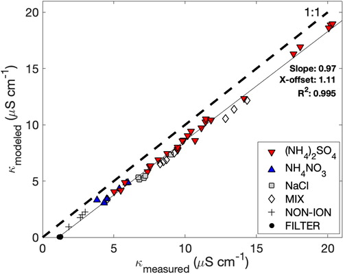
A soluble, but nonionic aerosol source (Nigrosine C.I. 50420, Sigma Aldrich) was used as a test point for comparison with the aerosol blanks, as a qualitative test for contributions from ambient gases. Nigrosine was selected instead of other test aerosol (e.g., polystyrene latex spheres, soot surrogates) because of operational difficulties with ingesting insoluble particles into the PILS at higher concentrations (e.g., Wonaschütz et al. 2019). The nigrosine results (Figure 2, NON-ION) followed the same closure relationship as the salt aerosols, with measurable ion contributions from NO₂^- and NH₄⁺. These species were also present in varying quantities in the samples associated with the salt aerosol cases (in the case of NH₄⁺ for the NH₄⁺-containing salts, it was in excess) and their contribution was attributed to gas phase NH₃ and NO_x (reacting in the PILS to form HONO), respectively. In contrast, there was a lack of NO₂^- and NH₄⁺ in the aerosol blanks and we attribute this difference to a lack of droplet growth sites in the absence of particle nuclei. We hypothesize that in this scenario, significantly reduced droplet surface area results in less efficient gas phase dissolution. This result may indicate that field blanks, collected using a particle filter, are a lower bound. A broader assessment of the use of particle filters and denuders on aerosol compositional measurements is relevant, especially for aircraft sampling, but beyond the scope of this work.

Time response

The temporal response of the PILS-conductivity measurement was assessed during instances where there was a step change in the aerosol sample, occurring when the ambient sample stream was diverted through a particle filter or was returned to ambient from the filter, creating an upward or downward step. The particle filter introduced a small additional pressure differential, which conveniently marked the transition time. Ten such transitions were extracted during lab aerosol testing and 16 transitions were assessed from flight data, usually at takeoff and landing (Figure 3).

Figure 3. Time response of the PILS-conductivity measurement assessed by evaluating the composite response of many step changes in aerosol during ground (red) and flight (black) operation. Response time is evaluated as the time to span 0.1 to 0.9 of the total step change in conductivity (Δκ) from a starting conductivity κ_init.

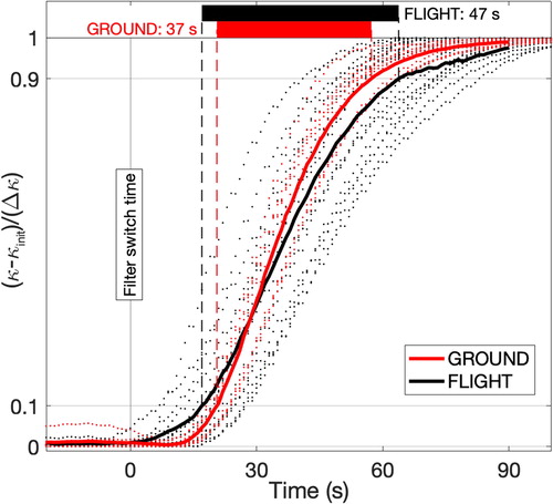
Each case shows the conductivity change from the initial condition normalized by the total conductivity change, creating a response curve with unit range. The time axis reflects the elapsed time since the step change was enacted. The cases shown in Figure 3 span a range of conductivity change (0.6–10.7 µS cm⁻¹) and there was no significant correlation found between the shape of the response curve and the magnitude of the conductivity change. In lieu of a theoretical model of the response curve, we use the time taken to span the range 0.1 to 0.9 (i.e., the center 80%) as a measure of the response time. The time delay can be corrected for (this is a standard practice for airborne operations); however, the response time derived here provides a measure for the degree of temporal smoothing that occurs. This unavoidably results in some filtering of short duration fluctuations, despite the conductivity cell itself being capable of far higher time resolution. The response time for in-flight tests was 47 ± 8 s with ground-based cases showing slightly quicker response (37 ± 4 s) and with less variability in the time delay. One contributing factor was that during ambient sampling in flight, the aerosol sampled by the PILS was not constant and so there was more uncertainty in the estimate of initial and final concentrations, unlike the laboratory generated aerosol where more stable conditions could be achieved.

The upstream and downstream roll off are suggestive of axial diffusion within the liquid lines, the debubbler, and a contribution from turbulent mixing within the PILS chamber. The longer downstream tail and the variability between the response curves is thought to be attributed to the impactor plate and liquid flow around the wick, which acts like a continuously mixed reservoir. The volume of this small liquid reservoir that surrounds the impactor (i.e., between the wash flow supply and the sample extraction) is not tightly controlled and may vary with environmental factors (e.g., pressure, temperature), aerodynamic flow around the impactor, and pump stability. Since the conductivity detection cell is not the limiting factor, further improvements in response time that do not involve increasing the liquid flow rate would require more substantial design changes to the impactor geometry and pumping system.

Ambient aerosol

Across the nineteen research flights conducted during CAMP²Ex, 1446 samples were collected from the PILS for offline IC analysis and 1384 of these samples were analyzed. The majority of the samples were collected below an altitude of 2 km, where aerosol mass concentrations were usually higher. An extensive portion of each flight was spent at high altitude (>6 km) for flight objectives related to remote sensing, transits and sampling mid-level clouds and convective detrainment. During the majority of these periods samples were not collected because aerosol mass was below or near the detection limit and instead, the continuously generated sample was diverted to waste. The conductivity measurement served as a primary real-time indicator of insufficient ionic mass together with companion aerosol instrumentation (e.g., AMS and LAS).

The measured conductivity was averaged (arithmetic mean) across the duration of each IC sample accounting for the time delay between the sample conductivity cell and the sample vial collection and the same closure analysis was performed as with the laboratory aerosol (Figure 4). Of the 1384 samples that were analyzed with IC, only 952 (69%) were included in the closure analysis. Remaining samples were rejected either because one or more species was not reported (24%), or because of quality assurance failures, including detection of bubbles (7%). For the ambient data, the model was augmented to include pressure-dependent background effects, κ₀ (e.g., from dissolved CO₂). The determination of κ₀ does not make use of speciated data (unlike other components of the conductivity model). Rather we make the simplifying assumption that κ₀ only varies with pressure. The N₂ zero (0.45 µS cm⁻¹), which we assume to represent a zero partial pressure limit for soluble gases, and the mean zero (1.1 µS cm⁻¹) at surface pressure were used to create a linear function with pressure. We note that even though the equilibrium for dissolved gases is proportional to the partial pressure, ion dissociation (and therefore conductivity) is pH dependent. However, since ions are required to change pH, the conductivity signal in these scenarios outweighs the significance of errors in modeling the background.

Figure 4. Comparison of measured and modeled conductivity (including background κ₀) for PILS data collected during CAMP²Ex. Data points highlighted in red indicate outliers (see text for details). The 1:1 line and best fit line to the data are both shown.

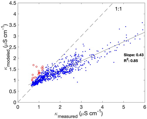
While there is appreciable scatter across the entire campaign dataset, a simple linear regression fit through the data indicates significant correlation (R²=0.85) and a fitted slope of 0.43, implying that at least half of the conductivity is not modeled. Samples whose modeled conductivity exceeds 110% of the measured conductivity (a 10% premium to reflect accuracy in measured ion concentrations) by 0.25 µS cm⁻¹ (a threshold estimate for uncertainty bounds in the conductivity measurement) are flagged as outlying samples (N = 17, Figure 4, highlighted red, not included in data fitting statistics) because the speciated ions would result in an implausibly high conductivity compared to the measurement (i.e., beyond the estimated uncertainty). For these samples, the conductivity measurement offers a diagnostic for unchecked positive artifacts (e.g., compromised sample vial, lab handling, chromatography errors). In contrast, the majority of samples fall below the 1:1 line and the deficit is attributed to missing, unmodeled ions.

To investigate this further, we define a conductivity deficit ${\kappa }^{\mathrm{*}}={\kappa }_{\mathit{meas}}-{\kappa }_{\mathit{model}}$ and calculate a charge imbalance $Z^{\mathrm{*}}=\sum z_x\left[X\right],$ where $z_x$ is the charge of ion x. We consider only samples with a deficit (i.e., ${\kappa }^{\mathrm{*}}>0$) and use a lower threshold ${\kappa }_{\mathit{meas}}>1.0$ (to discount samples near the baseline) such that the set includes 669 of the 952 used in the closure. 578 of these samples (86% of total) have a net negative charge, implying a cation deficit (Figure 5). A likely contributor to the cation deficit is H⁺ and, because of its high electrical mobility, it is an effective contributor to κ*. Charge-equivalent molar conductivity isopleths are shown in Figure 5 for H⁺ and other key ions or ion groups (NH₄⁺, CO₃^2-, HCO₃^-, R^n-; see Table 1), where R^n- corresponds to the range of charge-equivalent molar conductivity of anions associated with a selection of atmospherically relevant unmeasured organic anions (here we include acetate, formate, glycolate, malonate, succinate, glutarate, adipate, and maleate with conductivity data taken from Apelblat (2002)).

Figure 5. Charge imbalance (Z*) and conductivity deficit (κ*=κ_meas-κ_model) state space showing explanatory regions for the incomplete closure of the conductivity measurement with color shading indicating the sulfate concentration. Dashed curves represent isopleths of charge-equivalent molar conductivity for key species. The gray shaded region spans the isopleths of atmospherically relevant organic anions (see text for details).

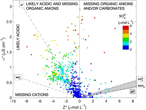
Data points in the region close to the H⁺ isopleth can be interpreted as the conductivity measurement supporting an ion imbalance attributed to H⁺ (acidic solutions caused by acidic aerosols entering the PILS and contributions from acidic gases of moderate to high solubility). Data points that exhibit a cation deficit but lie appreciably above the H⁺ isopleth cannot be explained by missing cations alone, since other cations are less mobile than H⁺ and so these points likely require unmeasured organic anions in addition to H⁺ derived from charge imbalance. For data points below the H⁺ isopleth, the cation deficit may be due to a mixture of H⁺ and other (less mobile) cations. Shown for reference, the NH₄⁺ isopleth represents the highest molar conductivity of the measured cations. Data points above this isopleth, but below the H⁺ isopleth are still indicative of acidic conditions but the acidity derived from ion imbalance represents an upper bound, and potentially an overestimate. Data with an anion deficit may be explained by organic anions and/or carbonates, but it is difficult to distinguish these because of similar molar conductivities.

Also indicated in Figure 5 is the sulfate concentration, which is assumed to be a likely contributor to acidity under ammonia-poor conditions. Data in the region close to the H⁺ isopleth generally show increasing [SO₄^2-] with increasing κ*, supportive of this attribution; however, there are also examples of (neutralized) high sulfate where additional species (e.g., organics) are required to explain κ* and likely underscores the diversity of sources encountered during the CAMP²Ex flights. A further notable point is that inferences on missing ions made from Figure 5 are not unique, despite utilizing the conductivity measurement (e.g., there could be multiple ways to explain charge imbalance and also achieve conductivity closure). The conductivity measurement does provide additional case-by-case support or opposition for ascribing charge imbalance to H⁺. As an auxiliary measurement, conductivity strengthens the ion balance method for qualitative assessment of acidity and offers additional constraints for species inputs to thermodynamic modeling of aerosol acidity.

Case study – Manila metropolitan area urban plume

The flight conducted on October 4th, 2019 (local date, takeoff October 3rd UTC) transected an airmass downwind of the Manila Metropolitan Area and is shown here to illustrate the fast time-response of the PILS conductivity measurement in a highly variable, complex mixture of urban aerosol sources. Immediately following the downwind transects, the aircraft was repositioned to conduct a “missed approach” at the Ninoy Aquino Manila International Airport, which facilitated low level in situ sampling to be carried out in close proximity to urban aerosol sources. During repositioning, the aircraft was required to climb to an altitude of approximately 2 km to conform with the airport traffic pattern and several penetrations of shallow cumulus occurred; consequently, the AMS and LAS instruments were switched to sample from the CVI inlet. Time series (Figure 6) show the structure of the plume observed during the downwind transects (01:10-02:15 UTC) and the missed approach (02:35-02:45 UTC), while the period encompassing the cloud sampling (02:24-02:30 UTC) has been removed for clarity.

Figure 6. Time series of selected parameters during a Manila plume crossing. (a) LAS-derived mass concentration (separated into sub-micrometer and super-micrometer components) and dry scattering coefficient at 550 nm, (b) speciated sub-micrometer mass concentration measured by the AMS, (c) speciated ionic mass concentrations measured by the PILS with offline IC, and (d) the baseline-corrected PILS conductivity (i.e., κ-κ₀). The gray shaded region indicates a period that was omitted for clarity, because of frequent cloud penetrations and instruments being switched to the CVI.

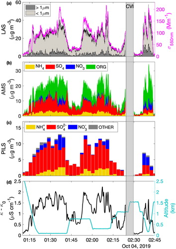
The number size distribution from the LAS is used to derive a particle volume distribution (assuming spherical particles). This is used to create estimates of sub-micrometer (i.e., PM₁) and super-micrometer aerosol mass concentration assuming particle effective density of 1.65 g cm⁻³ (using mean composition from the AMS) and 2 g cm⁻³, respectively (Figure 6a). Super-micrometer integrated volume estimates are smoothed with a 30 s running mean to mitigate limitations with counting statistics. Comparison with the dry scattering coefficient at 550 nm shows agreement in the structure of the plume and a mass-scattering efficiency of 4-6, which is on the upper bound of established ranges for organic particles (Hand and Malm 2007). Speciated PM₁ measurements from the AMS (NH₄, SO₄, NO₃ and total organic mass (ORG), Figure 6b) mirror the microphysically derived mass concentration. Good agreement is found between NH₄⁺, SO₄^2-, and NO₃^- ion concentrations derived from the PILS samples (Figure 6c) and their respective equivalent species in the AMS. The remaining seven ions from the PILS are combined and reported as “other” and are a minor component of the mass inferred from PILS. A notable compositional shift was observed during repeated sampling that took place at an altitude just above the boundary layer (01:10-01:18, 01:42-01:52, 02:13-02:20 UTC) where overall concentrations were lower and the aerosol was dominated by SO₄, with incomplete neutralization by NH₄. An increased fraction of organic mass was observed at the missed approach and at several instances during the downwind transect (notably around 01:37 and 02:10 UTC) and these occasions also were marked by higher NO₃. Notably, the PILS also captured these periods in the NO₃^- despite their short duration, although it is acknowledged that a fraction of the PILS NO₃^- may also be from gas phase contributions. Emissions and secondary sources are not discussed further; rather we showcase the structure and changing composition to illustrate that this was a complex plume environment.

The measured conductivity is shown across the same time period (Figure 6d) with the (modeled) background subtracted (i.e., κ-κ₀). The improvement in the temporal resolution over the (150 s) PILS speciated ions is clearly apparent and it captures many of the fine-scale peaks evident in the AMS, LAS-estimated mass, and dry scattering data. The comparison illustrates the potential of this technique to augment the detailed (but labor-intensive) information gained from batch samples run offline with IC. During periods of un-neutralized SO₄ (e.g., 01:40–01:50 UTC), the reduction in conductivity is less pronounced compared to the reduction in mass, which is consistent with acidic conditions and the contribution of H⁺ to conductivity. During periods of enhanced organic mass (e.g., the missed approach) the increase in conductivity is not as strong as is observed during other periods of comparable mass and may indicate that a significant fraction of the organic mass is not ionic, a likely scenario for freshly emitted urban aerosols.

Summary

A flow-through conductivity cell has been incorporated into a PILS to provide a continuous online measurement in support of batch samples analyzed offline using IC. A primary advantage of the technique is that it is nondestructive and preserves the integrity of the sample for subsequent offline analysis. At minimum, it provides a simple, low cost diagnostic tool for continuous evaluation of the PILS; this is needed for aircraft operation where changing environmental conditions can make PILS operation challenging. The PILS-conductivity measurement has been shown to demonstrate successful closure with nebulized single-salt aerosols and offers additional supporting information about likely missing ions in the case of more complex ambient aerosol mixtures. A particularly relevant example of this is to assist in the identification of acidic aerosols. The PILS-conductivity measurement also augments the temporal capability of the PILS for the detection of ionic species, beyond that which is obtained from analyzing batch IC samples offline. Analysis of the time response suggests that the measurement is capable of capturing sub-minute variability and examination of its performance during sampling of highly variable concentrations and composition demonstrates compelling structural agreement with other independent measurements of aerosol mass.

Disclosure statement

The authors declare no conflicts of interest, financial interests or benefits.

Additional information

Funding

This research was funded by NASA's Radiation Sciences Program and authors from the University of Arizona acknowledge support from NASA grant 80NSSC18K0148. This work was funded in part by the ACTIVATE Earth Venture Suborbital-3 (EVS-3) investigation, which is supported by NASA’s Earth Science Division and managed through the Earth System Science Pathfinder Program Office. We wish to thank the pilots and flight crew of the NASA Wallops Flight Facility P-3 aircraft for their support throughout the CAMP²Ex field campaign. We would also like to recognize the assistance from the NASA Ames Earth Science Project Office (ESPO) and facilities personnel at the Clark International Airport in Pampanga, Philippines. Finally, we would like to thank students and staff at the Manila Observatory for help in our field laboratory and we thank the two anonymous reviewers for their constructive feedback.

References

- Agmon, N. 1995. The Grotthuss Mechanism. Chem. Phys. Lett. 244 (5–6):456–62. doi:10.1016/0009-2614(95)00905-J.
- Allan, J. D., A. E. Delia, H. Coe, K. N. Bower, M. R. Alfarra, J. L. Jimenez, A. M. Middlebrook, F. Drewnick, T. B. Onasch, M. R. Canagaratna, et al. 2004. A generalised method for the extraction of chemically resolved mass spectra from Aerodyne aerosol mass spectrometer data. J. Aerosol Sci. 35 (7):909–22. doi:10.1016/j.jaerosci.2004.02.007.
- Apelblat, A. 2002. Dissociation constants and limiting conductances of organic acids in water. J. Mol. Liq. 95 (2):99–145. doi:10.1016/S0167-7322(01)00281-1.
- Bešter-Rogač, M., M. Tomšič, J. Barthel, R. Neueder, and A. Apelblat. 2002. Conductivity studies of dilute aqueous solutions of oxalic acid and neutral oxalates of sodium, potassium, cesium, and ammonium from 5 to 35° C. J. Sol. Chem. 31 (1):1–18. doi:10.1023/A:1014805417286.
- Beyersdorf, A. J., L. D. Ziemba, G. Chen, C. A. Corr, J. H. Crawford, G. S. Diskin, R. H. Moore, K. L. Thornhill, E. L. Winstead, and B. E. Anderson. 2016. The impacts of aerosol loading, composition, and water uptake on aerosol extinction variability in the Baltimore–Washington, DC region. Atmos. Chem. Phys. 16 (2):1003–15. doi:10.5194/acp-16-1003-2016.
- Brock, C. A., P. K. Hudson, E. R. Lovejoy, A. Sullivan, J. B. Nowak, L. G. Huey, O. R. Cooper, D. J. Cziczo, J. de Gouw, F. C. Fehsenfeld, et al. 2004. Particle characteristics following cloud‐modified transport from Asia to North America. J. Geophys. Res 109 (D23); Article number D23S26. doi:10.1029/2003JD004198.
- de Grotthuss, C. J. T. 1806. Mémoire sur la décomposition de l'eau et des corps qu'elle tient en dissolution à l'aide de l'álectricité galvanique. Ann. Chim. Phy. (Paris) 58:54–74.
- Guo, H., A. P. Sullivan, P. Campuzano-Jost, J. C. Schroder, F. D. Lopez-Hilfiker, J. E. Dibb, J. L. Jimenez, J. A. Thornton, S. S. Brown, A. Nenes, et al. 2016. Fine particle pH and the partitioning of nitric acid during winter in the northeastern United States. J. Geophys. Res. Atmos. 121 (17):10,355–355., 2016: doi:10.1002/2016JD025311.
- Gustafson, H., and A. S. Behrman. 1939. Determination of total dissolved solids in water by electrical conductivity. Ind. Eng. Chem. Anal. Ed. 11 (7):355–7. doi:10.1021/ac50135a001.
- Hand, J. L., and W. C. Malm. 2007. Review of aerosol mass scattering efficiencies from ground‐based measurements since 1990. J. Geophys. Res. 112 (D16); Article number D16203 doi:10.1029/2007JD008484.
- Hecobian, A., X. Zhang, M. Zheng, N. Frank, E. S. Edgerton, and R. J. Weber. 2010. Water-soluble organic aerosol material and the light-absorption characteristics of aqueous extracts measured over the Southeastern United States. Atmos. Chem. Phys. 10 (13):5965–77.
- Hennigan, C. J., J. Izumi, A. P. Sullivan, R. J. Weber, and A. Nenes. 2015. A critical evaluation of proxy methods used to estimate the acidity of atmospheric particles. Atmos. Chem. Phys. 15 (5):2775–90. doi:10.5194/acp-15-2775-2015.
- Hersey, S. P., J. S. Craven, A. R. Metcalf, J. Lin, T. Lathem, K. J. Suski, J. F. Cahill, H. T. Duong, A. Sorooshian, H. H. Jonsson, et al. 2013. Composition and hygroscopicity of the Los Angeles aerosol: CalNex. J. Geophys. Res. Atmos. 118 (7):3016–36. doi:10.1002/jgrd.50307.
- Hersey, S. P., J. S. Craven, K. A. Schilling, A. R. Metcalf, A. Sorooshian, M. N. Chan, R. C. Flagan, and J. H. Seinfeld. 2011. The Pasadena Aerosol Characterization Observatory (PACO): chemical and physical analysis of the Western Los Angeles basin aerosol. Atmos. Chem. Phys. 11 (15):7417–43. doi:10.5194/acp-11-7417-2011.
- Kenseth, C. M., Y. Huang, R. Zhao, N. F. Dalleska, J. C. Hethcox, B. M. Stoltz, and J. H. Seinfeld. 2018. Synergistic O3 + OH oxidation pathway to extremely low-volatility dimers revealed in β-pinene secondary organic aerosol. Proc. Natl. Acad. Sci. USA. 115 (33):8301–6. doi:10.1073/pnas.1804671115.
- Lee, Y. ‐N., R. Weber, Y. Ma, D. Orsini, K. Maxwell‐Meier, D. Blake, S. Meinardi, et al. 2003. Airborne measurement of inorganic ionic components of fine aerosol particles using the particle‐into‐liquid sampler coupled to ion chromatography technique during ACE‐Asia and TRACE‐P. J. Geophys. Res. 108 (D23); Article number 8646. doi:10.1029/2002JD003265.
- Lee, T., X.-Y. Yu, S. M. Kreidenweis, W. C. Malm, and J. L. Collett. 2008. Semi-continuous measurement of PM2. 5 ionic composition at several rural locations in the United States. Atmos. Environ. 42 (27):6655–69. doi:10.1016/j.atmosenv.2008.04.023.
- Lewis, E. 1980. The practical salinity scale 1978 and its antecedents. IEEE J. Oceanic Eng. 5 (1):3–8. doi:10.1109/JOE.1980.1145448.
- Li, Z., P. K. Hopke, L. Husain, S. Qureshi, V. A. Dutkiewicz, J. J. Schwab, F. Drewnick, and K. L. Demerjian. 2004. Sources of fine particle composition in New York city. Atmos. Environ. 38 (38):6521–9. doi:10.1016/j.atmosenv.2004.08.040.
- McCleskey, R. B. 2011. Electrical conductivity of electrolytes found in natural waters from (5 to 90) C. J. Chem. Eng. Data 56 (2):317–27. doi:10.1021/je101012n.
- McCleskey, R. B., D. K. Nordstrom, and J. N. Ryan. 2012b. Comparison of electrical conductivity calculation methods for natural waters. Limnol. Oceanogr. Methods 10 (11):952–67. doi:10.4319/lom.2012.10.952.
- McCleskey, R. B., D. K. Nordstrom, J. N. Ryan, and J. W. Ball. 2012a. A new method of calculating electrical conductivity with applications to natural waters. Geochim. Cosmochim. Acta 77:369–82. doi:10.1016/j.gca.2011.10.031.
- McNaughton, C. S., A. D. Clarke, S. G. Howell, M. Pinkerton, B. Anderson, L. Thornhill, C. Hudgins, E. Winstead, J. E. Dibb, E. Scheuer, et al. 2007. Results from the DC-8 Inlet Characterization Experiment (DICE): Airborne versus surface sampling of mineral dust and sea salt aerosols. Aerosol Sci. Technol. 41 (2):136–59. doi:10.1080/02786820601118406.
- Murphy, D. M., D. J. Cziczo, K. D. Froyd, P. K. Hudson, B. M. Matthew, A. M. Middlebrook, R. E. Peltier, A. Sullivan, D. S. Thomson, and R. J. Weber. 2006. Single‐particle mass spectrometry of tropospheric aerosol particles. J. Geophys. Res. 111 (D23); Article number D23S32. doi:10.1029/2006JD007340.
- Nah, T., H. Guo, A. P. Sullivan, Y. Chen, D. J. Tanner, A. Nenes, A. Russell, N. L. Ng, L. G. Huey, and R. J. Weber. 2018. Characterization of aerosol composition, aerosol acidity, and organic acid partitioning at an agriculturally intensive rural southeastern US site. Atmos. Chem. Phys. 18 (15):11471–91. doi:10.5194/acp-18-11471-2018.
- Orsini, D. A., Y. Ma, A. Sullivan, B. Sierau, K. Baumann, and R. J. Weber. 2003. Refinements to the particle-into-liquid sampler (PILS) for ground and airborne measurements of water soluble aerosol composition. Atmos. Environ. 37 (9–10):1243–59. doi:10.1016/S1352-2310(02)01015-4.
- Peltier, R. E., A. P. Sullivan, R. J. Weber, A. G. Wollny, J. S. Holloway, C. A. Brock, J. A. De Gouw, and E. L. Atlas. 2007. No evidence for acid‐catalyzed secondary organic aerosol formation in power plant plumes over metropolitan Atlanta, Georgia. Geophys. Res. Lett. 34 (6); Letter number L06801. doi:10.1029/2006GL028780.
- Prieto, F., E. Barrado, M. Vega, and L. Deban. 2001. Measurement of electrical conductivity of wastewater for fast determination of metal ion concentration. Russ. J. Appl. Chem. 74 (8):1321–4. doi:10.1023/A:1013710413982.
- Rastogi, N., M. M. Oakes, J. J. Schauer, M. M. Shafer, B. J. Majestic, and R. J. Weber. 2009. New technique for online measurement of water-soluble Fe (II) in atmospheric aerosols. Environ. Sci. Technol. 43 (7):2425–30. doi:10.1021/es8031902.
- Robinson, R. A., and R. H. Stokes. 2002. Electrolyte solutions. Courier Corporation, 126–9, 133–43.
- Saarnio, K., K. Teinilä, S. Saarikoski, S. Carbone, S. Gilardoni, H. Timonen, M. Aurela, and R. Hillamo. 2013. Online determination of levoglucosan in ambient aerosols with particle-into-liquid sampler-high-performance anion-exchange chromatography-mass spectrometry (PILS-HPAEC-MS). Atmos. Meas. Tech. 6 (10):2839–49. doi:10.5194/amt-6-2839-2013.
- Shingler, T., S. Dey, A. Sorooshian, F. J. Brechtel, Z. Wang, A. Metcalf, M. Coggon, J. Mülmenstädt, L. M. Russell, H. H. Jonsson, et al. 2012. Characterization and airborne deployment of a new counterflow virtual impactor inlet. Atmos. Meas. Tech. Discuss. 5 (1):1515–41. doi:10.5194/amtd-5-1515-2012.
- Sorooshian, A., F. J. Brechtel, Y. Ma, R. J. Weber, A. Corless, R. C. Flagan, and J. H. Seinfeld. 2006a. Modeling and characterization of a particle-into-liquid sampler (PILS). Aerosol Sci. Technol. 40 (6):396–409. doi:10.1080/02786820600632282.
- Sorooshian, A., E. Crosbie, L. C. Maudlin, J.-S. Youn, Z. Wang, T. Shingler, A. M. Ortega, S. Hersey, and R. K. Woods. 2015. Surface and airborne measurements of organosulfur and methanesulfonate over the western United States and coastal areas. J. Geophys. Res. Atmos. 120 (16):8535–48. doi:10.1002/2015JD023822.
- Sorooshian, A., S. M. Murphy, S. Hersey, H. Gates, L. T. Padro, A. Nenes, F. J. Brechtel, H. Jonsson, R. C. Flagan, and J. H. Seinfeld. 2008. Comprehensive airborne characterization of aerosol from a major bovine source. Atmos. Chem. Phys. 8 (17):5489–520. doi:10.5194/acp-8-5489-2008.
- Sorooshian, A., N. L. Ng, A. W H. Chan, G. Feingold, R. C. Flagan, and J. H. Seinfeld. 2007. Particulate organic acids and overall water‐soluble aerosol composition measurements from the 2006 Gulf of Mexico Atmospheric Composition and Climate Study (GoMACCS). J. Geophys. Res.: Atmos. 112 (D13); Article number D13201.
- Sorooshian, A., V. Varutbangkul, F. J. Brechtel, B. Ervens, G. Feingold, R. Bahreini, S. M. Murphy, J. S. Holloway, E. L. Atlas, G. Buzorius, et al. 2006b. Oxalic acid in clear and cloudy atmospheres: Analysis of data from International Consortium for Atmospheric Research on Transport and Transformation 2004. J. Geophys. Res. 111 (D23); Article number D23S45. doi:10.1029/2005JD006880.
- Spitzer, P., B. Rossi, Y. Gaignet, S. Mabic, and U. Sudmeier. 2005. New approach to calibrating conductivity meters in the low conductivity range. Accred. Qual. Assur. 10 (3):78–81. doi:10.1007/s00769-004-0880-4.
- Sullivan, A. P., R. J. Weber, A. L. Clements, J. R. Turner, M. S. Bae, and J. J. Schauer. 2004. A method for on‐line measurement of water‐soluble organic carbon in ambient aerosol particles: Results from an urban site. Geophys. Res. Lett. 31 (13); Letter number L13105. doi:10.1029/2004GL019681.
- Surratt, J. D., J. H. Kroll, T. E. Kleindienst, E. O. Edney, M. Claeys, A. Sorooshian, N. L. Ng, J. H. Offenberg, M. Lewandowski, M. Jaoui, et al. 2007. Evidence for organosulfates in secondary organic aerosol. Environ. Sci. Technol. 41 (2):517–27. doi:10.1021/es062081q.
- Walton, N. R. G. 1989. Electrical conductivity and total dissolved solids—what is their precise relationship? Desalination 72 (3):275–92. doi:10.1016/0011-9164(89)80012-8.
- Weber, R. J., S. Lee, G. Chen, B. Wang, V. Kapustin, K. Moore, A. D. Clarke, L. Mauldin, E. Kosciuch, C. Cantrell, et al. 2003. New particle formation in anthropogenic plumes advecting from Asia observed during TRACE‐P. J. Geophys. Res. 108 (D21); Article number 8814. doi:10.1029/2002JD003112.
- Weber, R. J., D. Orsini, Y. Daun, Y.-N. Lee, P. J. Klotz, and F. Brechtel. 2001. A particle-into-liquid collector for rapid measurement of aerosol bulk chemical composition. Aerosol Sci. Technol. 35 (3):718–27. doi:10.1080/02786820152546761.
- Wonaschuetz, A., T. Haller, E. Sommer, L. Witek, H. Grothe, and R. Hitzenberger. 2019. Collection of soot particles into aqueous suspension using a particle-into-liquid sampler. Aerosol Sci. Technol. 53 (1):21–8. doi:10.1080/02786826.2018.1540859.
- Wonaschuetz, A., A. Sorooshian, B. Ervens, P. Y. Chuang, G. Feingold, S. M. Murphy, J. de Gouw, C. Warneke, and H. H. Jonsson. 2012. Aerosol and gas re‐distribution by shallow cumulus clouds: An investigation using airborne measurements. J. Geophys. Res. 117 (D17); Article number D17202. doi:10.1029/2012JD018089.
- Xue, J., Z. Yuan, A. K. H. Lau, and J. Z. Yu. 2014. Insights into factors affecting nitrate in PM2. 5 in a polluted high NOx environment through hourly observations and size distribution measurements. J. Geophys. Res. Atmos. 119 (8):4888–902. doi:10.1002/2013JD021108.
- Youn, J.-S., E. Crosbie, L. C. Maudlin, Z. Wang, and A. Sorooshian. 2015. Dimethylamine as a major alkyl amine species in particles and cloud water: Observations in semi-arid and coastal regions. Atmos. Environ. (1994) 122:250–8. doi:10.1016/j.atmosenv.2015.09.061.
- Zhang, X., N. F. Dalleska, D. D. Huang, K. H. Bates, A. Sorooshian, R. C. Flagan, and J. H. Seinfeld. 2016. "Time-resolved molecular characterization of organic aerosols by PILS + UPLC/ESI-Q-TOFMS. Atmos. Environ. 130:180–9. doi:10.1016/j.atmosenv.2015.08.049.