Quantifying errors in the aerosol mixing-state index based on limited particle sample size

Abstract

This study evaluates the error that is introduced in quantifying observed aerosol mixing states due to a limited particle sample size. We used the particle-resolved model PartMC-MOSAIC to generate a scenario library that encompasses a large number of reference particle populations with a wide range of mixing states quantified by the mixing-state index χ. We stochastically sub-sampled these particle populations using sample sizes of 10 to 10,000 particles and recalculated χ based on the sub-samples. The finite sample size led to a consistent overestimation of χ, with the 95% confidence intervals ranging from −70 to 30 percentage points for sample sizes of 10 particles, and decreasing to ±10 percentage points for sample sizes of 10,000 particles. These findings were experimentally confirmed with single-particle measurements from the Pittsburgh area using a soot-particle aerosol mass spectrometer.

Copyright © 2020 American Association for Aerosol Research

EDITOR:

• Kihong Park

1. Introduction

Atmospheric aerosols are evolving mixtures of different chemical species (Prather, Hatch, and Grassian 2008). The term “aerosol mixing state” is commonly used to describe how different chemical species are distributed throughout a particle population (Winkler 1973; Riemer et al. 2019). Aerosol mixing state influences the particles’ reactivity (Ryder et al. 2014), their optical properties (Moffet and Prather 2009; Lesins, Chylek, and Lohmann 2002), their hygroscopicity (Sullivan et al. 2009; Ching et al. 2017), and their propensity to serve as ice nuclei (Beydoun, Polen, and Sullivan 2017; Knopf and Alpert 2013). Hence, to predict aerosol impacts on atmospheric chemistry and climate, it is important to account for mixing state (Riemer et al. 2019); and this motivates efforts to determine mixing state from ambient observations (Healy et al. 2014; O’Brien et al., 2015; Ye et al. 2018) and via modeling (Riemer et al. 2009; Riemer and West 2013; Ching, Riemer, and West 2016).

The terms “internal” and “external” mixture qualitatively describe mixing state. A population is considered fully internally mixed if each individual particle consists of the same species mixtures, while an external mixture implies that the different aerosol species reside in separate particles. Most ambient aerosol populations do not fit into either category, but resemble both internal and external mixtures to a degree. Often the term “mixing state” is applied to particles in a given size range, for example the accumulation mode or the coarse mode. This choice depends on the aerosol sampling instrumentation specifications or the science question being addressed. It is also important to be aware that mixing state as defined here does not capture the full potential diversity of particle populations, as the particle morphology (e.g., core-shell, well-mixed) can add additional diversity. In this article, we will only consider mixing state as defined above, which is also termed the “chemical mixing state” in Riemer et al. (2019).

For a quantitative description of aerosol mixing state, the mixing-state index χ has been introduced (Riemer and West 2013), which can be calculated based on the particles’ species mass fractions. This scalar quantity ranges from 0 to 100% for fully external to internal mixtures, respectively. Several field studies have used this index to quantify mixing states for different ambient environments using sophisticated single-particle measurement techniques, including electron microscopy and X-ray spectroscopy (O’Brien et al., 2015), and mass spectrometry (Healy et al. 2013). These observations confirm that mixing states in the ambient atmosphere are neither completely internally nor externally mixed but rather exist on a spectrum in between those limiting cases with characteristic temporal and spatial variability. For example, a study by Healy et al. (2014) for the MEGAPOLI campaign in Paris, France, revealed that the aerosol in Paris was estimated to be 59% internally mixed on average, with more external mixtures during the daytime when primary emissions from traffic and woodburning were present, and more internal mixtures during the night when ammonium nitrate formation prevailed. Healy et al. (2014) used single-particle aerosol time-of-flight mass spectrometry (ATOFMS) data for their study. Ye et al. (2018) quantified the spatial variation of χ for the city of Pittsburgh on a neighborhood scale with a mobile measurement platform using single-particle measurements from a soot-particle aerosol mass spectrometer (SP-AMS) and found the lowest values (36%) close to an interstate highway and the highest values (76%) in rural or suburban regions.

The mixing-state index χ is based on species diversity measures (Riemer and West 2013), which have been extensively used and developed in ecology and related fields. See Daly, Baetens, and Baets (2018) for an excellent overview and Sherwin and Prat I Fornells (2019) for a discussion of the history. Within ecology it is well-known that undersampling can result in inaccurate and biased estimates of diversity measures (Beck and Schwanghart 2010; Beck, Holloway, and Schwanghart 2013) and the performance of different statistical methods has been studied for realistic scenarios (Butturi-Gomes et al. 2017; Brocklehurst, Day, and Fröbisch 2018). In response, better estimators have been proposed that are based on the discovery rate of new species (Chao, Wang, and Jost 2013; Chao and Jost 2015; Haegeman et al. 2013), measures such as pairwise dissimilarities (Marion 2016) have been used as alternatives, and Bayesian estimators have been developed (Marion, Fordyce, and Fitzpatrick 2018).

Just as undersampling is a problem in ecology, measurements of atmospheric aerosols inherently sample a finite number of particles to estimate the mixing state and associated metrics. These finite samples range from a few hundred to many thousands of particles, depending on the instrumentation. For example, O’Brien et al. (2015) utilized electron microscopy and X-ray spectroscopy methods to analyze particle samples from the 2010 Carbonaceous Aerosols and Radiative Effects study with sample sizes ranging from several hundred to several thousand particles. Ye et al. (2018) used single-particle mass spectrometry with sample sizes on the order of tens of thousand of particles. Unfortunately, we cannot directly apply the improved diversity estimators developed in ecology (Chao and Jost 2015) because they use the fact that species abundance is measured by sampling individuals in the species, a concept that does not readily transfer to chemical measurements.

The question arises of how large a particle sample size must be to adequately represent the mixing state of an atmospheric aerosol. Using a large ensemble of simulated aerosol populations generated with a particle-resolved model, the goal of this article is to quantify errors in determining χ introduced by limited-size particle samples. Since the “true” value of χ is not known when making observations in practice, we also provide confidence intervals around the measured χ values for different sample sizes.

2. Methods

2.1. Calculating mixing-state index χ

The mixing-state index χ by Riemer and West (2013) provides a rigorous definition of aerosol mixing state. It is given by the affine ratio of the diversity metrics D_α and D_γ as (1) $$\chi =\frac{D_{\alpha }-1}{D_{\gamma }-1}.$$(1)

The diversity metrics, in turn, are defined as follows. First, the particle mixing entropies H_i need to be calculated for each particle based on the particle species mass fractions (2) $$H_i=\sum _{a=1}^A-p_i^a\hspace{0.17em}\text{ln}\hspace{0.17em}{p}_i^a,$$(2) where A is the number of distinct aerosol species, and $p_i^a$ is the mass fraction of species a in particle i. The particle diversities $D_i=\hspace{0.17em}\text{exp}\hspace{0.17em}(H_i)$ give the effective number of species in each particle, which is equal to the number of physical species if they are all present in equal proportions, and less otherwise.

The particle H_i values are then averaged (mass-weighted) over the entire population to give H_α, and finally the average particle species diversity D_α, by (3) $$H_{\alpha }=\sum _{i=1}^{N_{\mathit{p}}}{p}_i{H}_i,$$(3) (4) $$D_{\alpha }=e^{H_{\alpha }},$$(4) where N_p is the total number of particles in the population, and p_i is the mass fraction of particle i in the population. D_α is the mean particle diversity, which gives the mean effective number of species over all particles in the population.

Lastly, the bulk diversity D_γ is defined by (5) $$H_{\gamma }=\sum _{a=1}^A-p^a\hspace{0.17em}\text{ln}\hspace{0.17em}{p}^a,$$(5) (6) $$D_{\gamma }=e^{H_{\gamma }}.$$(6)

This is the total diversity of the population, which is the effective number of species in the aerosol bulk.

Importantly, the definition of “species” depends on the application or the instrumentation used to determine mass fractions. In some previous studies, elemental species have been used (O’Brien et al., 2015; Fraund et al. 2017; Bondy et al. 2018), while others used molecular species (Healy et al. 2014; Ye et al. 2018) or species groups (Dickau et al. 2016; Ching et al. 2017; Hughes et al. 2018). To make our results comparable to Ye et al. (2018) (who observed organics, nitrate, sulfate, chloride and black carbon, as detected by the soot-particle aerosol mass spectrometer), we chose the aerosol model species that constitute the dry aerosol mass, such as ammonium, sulfate, nitrate, black carbon, as well as several organic species, with the addition of dust and sodium chloride. Note that the soot-particle aerosol mass spectrometer cannot measure dust and sodium chloride. Aerosol water is excluded from our calculations. While our scenario library includes coarse-mode particles, we only included sub-micron particles in our calculations for χ, since this is the relevant size range for ambient measurements using AMS instruments.

2.2. PartMC-MOSAIC model description

PartMC-MOSAIC is a unique modeling tool to simulate aerosol mixing state and its impacts under a wide variety of conditions. With this tool, each particle can be represented explicitly, allowing for accurate calculations of single-particle species mass fraction This is in contrast to other common aerosol modeling techniques which represent averages of particle composition over certain size ranges rather than per-particle composition (Riemer et al. 2019). A detailed description of PartMC-MOSAIC is given in Riemer et al. (2009). In brief, PartMC (Particle-resolved Monte Carlo) is a box model that explicitly resolves composition on a per-particle level within a well-mixed computational volume representative of a much larger air parcel. The evolution of the particle population—due to Brownian coagulation, emission and dilution—is tracked throughout the simulation using the Monte Carlo approach. PartMC is coupled to MOSAIC (Model for Simulating Aerosol Interactions and Chemistry) (Zaveri et al. 2008) which models gas-phase chemistry and gas-particle partitioning (condensation processes). MOSAIC consists of four modules: (1) the gas-phase photochemistry mechanism CBM-Z (Zaveri and Peters 1999), (2) the Multicomponent Taylor Expansion Method (MTEM) (Zaveri, Easter, and Wexler 2005b), (3) the Multicomponent Equilibrium Solver for Aerosols (MESA) for intraparticle solid-liquid partitioning (Zaveri, Easter, and Peters 2005a), and (4) the Adaptive Step Time-split Euler Method (ASTEM) for dynamic gas-particle partitioning (Zaveri et al. 2008). To simulate secondary organic aerosol (SOA) the SORGAM scheme is used (Schell et al. 2001). MOSAIC treats all locally and globally important gas and aerosol species including a total of 77 gaseous species and 19 aerosol species including ${\text{SO}}_4^{2-},{\text{HSO}}_4^{-},{\text{NO}}_3^{-},{\text{Cl}}^{-},{\text{CO}}_3^{-},{\text{NH}}_4^{+},{\text{Na}}^{+},{\text{Ca}}^{2+},$ other inorganic mass (representing crustal material), black carbon (BC), primary organic aerosol (POA) and SOA.

2.3. Ensemble of scenarios and sampling technique

To generate confidence intervals for χ for a wide range of conditions, we made use of a scenario library comprising 1000 different PartMC-MOSAIC scenarios (Hughes et al. 2018). All scenarios used a simulation time of 24 h, starting at 6:00 AM local time, with output saved every hour. Each simulation was run using 100,000 computational particles, producing a high-resolution representation of aerosol mixing state. Twenty-four input parameters (temperature, relative humidity, latitude, gas phase emission rates, emission rates, size parameters and composition of primary aerosol particles, including carbonaceous particles, sea salt, and mineral dust) were varied between scenarios to allow for large variations in mixing-state evolution. The scenario inputs were generated using Latin hypercube sampling to provide efficient sampling across the high-dimensional input parameter space. The entire scenario library generated 24,000 distinct reference particle populations (24 h × 1000 scenarios) (Gasparik et al. 2020). For each reference population we calculated the reference value χ_ref of the mixing-state index.

To mimic the sampling process used in single-particle field measurements, we subsampled each reference population without replacement using different sample sizes ($N=10,100,1000,10,000$). To determine confidence intervals we repeated each subsampling 1000 times, which resulted in 24,000,000 sampled particle populations (24 h × 1000 scenarios × 1000 samples) for each sample size N. For each sampled population we recalculated χ using only the particles in the sample and we denoted these χ values as ${\chi }_{\text{samp}}^N.$ Similarly, $D_{\alpha ,\mathrm{s}\mathrm{amp}}^N$ and $D_{\gamma ,\mathrm{s}\mathrm{amp}}^N$ are the α- and γ-diversities computed used only the sampled particles.

It is important to note that even the large number of 100,000 computational particles still represents an—albeit large—subsample of the “true” limiting population with a (near-)infinite number of particles. The key point is that the error between the 100,000 particle sample and the true population is expected to be much smaller than the error between our largest subsample (10,000 particles) and the true population. This is a reasonable assumption as the error scales with $1/\sqrt{N},$ meaning that the error for the 100,000-particle sample is a factor of $\sqrt{10}$ smaller than that of the 10,000-sample. To maintain this $\sqrt{10}$ factor, we limit the largest sample to 10% of the size of our reference population.

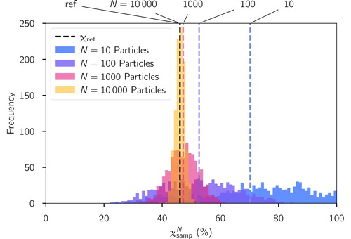
Figure 1 illustrates this process for one single reference population. In this case, χ_ref was 46%. Sampling this population with only 10 particles produced a broad range of ${\chi }_{\text{samp}}^{10}$ values from 20 to 100%. This range narrowed progressively as N increased, resulting in a range of 41 to 50% for a sample size of 10,000 particles. Another important result is that for small sample sizes, ${\chi }_{\text{samp}}^N$ overestimates χ_ref. In Section 3, we will see that this positive bias is a consistent result of the sampling process that can be explained with the fact that on average a sub-population overestimates D_α and underestimates D_γ. A rigorous proof is provided in Section 4.

Figure 1. Frequency distribution of ${\chi }_{\text{samp}}^N$ for one example population (${\chi }_{\text{ref}}=46\%$) and different sample sizes. For each sample size, the sampling process was repeated 1000 times. The dashed colored lines correspond to the average ${\overline{\chi }}_{\text{samp}}^N$ for the specified sample size.

2.4. Experimental determination of χ using observations in Pittsburgh

To provide experimental confirmation for the particle-resolved modeling results, a similar analysis was conducted using field data from Ye et al. (2018). In this study, aerosol samples were collected using the single-particle mode of a soot-particle aerosol mass spectrometer on a mobile platform throughout the city of Pittsburgh, PA.

The seven major particle clusters or types identified in the Pittsburgh mobile sampling data set were classified as: a sulfate-rich inorganic class that also contained OA and nitrate measured in the summer, a nitrate-domoinated class with small amounts of sulfate and little OA measured in the winter, less-oxidized hydrocarbon-like organics (HOA) associated with vehicle emissions, less-oxidized cooking-like organic aerosol (COA) associated with restaurant emissions, black carbon-dominated with small amounts of OA or inorganics, more-oxygeneated OA rich, and less-oxygeneated OA rich (Ye et al. 2018). The later two OA-rich classes contained small amounts of inorganics. Differences in particle composition and mixing state and of these properties as a function of particle size were observed in different sampled environments that included: in highly trafficked tunnels, on highways, an urban area with high traffic density, and on a road through a large park. Other specific environments that produced unique particle mixing states included: inside a restaurant plume (COA dominated), downtown with high restaurant density (mixture of COA, inorganics, and HOA), and a suburban residential area with low restaurant density (diverse mixture of inorganics, OA, COA, and HOA) (Ye et al. 2018).

Three aerosol samples were used for the analysis here including the sample collected in Pittsburgh downtown (∼11,000 particles), at the Carnegie Mellon University (CMU) urban campus in the summer (∼15,000 particles) and at the CMU campus in the winter (∼47,000 particles). Aerosols collected in Pittsburgh downtown were chosen to represent samples from regions that are in close proximity to sources of primary particles, while the CMU campus represents an urban background. Aerosol populations collected in Pittsburgh downtown were a combination of six visits to downtown, and the sampling time for each visit ranged between 30 min and 1 h. Aerosol populations collected on CMU campus were aggregated over several hours to a day. Based on the single-particle spectra of the three populations, per-particle mass fractions were determined and mixing state indices χ_ref were calculated for each population. Five species are considered for calculations of the mixing state index: organics, nitrate, sulfate, chloride and black carbon. Ammonium is not considered due to the large interference from the water signal in the mass spectra in the single-particle aerosol mass spectrometer. For more details about the method of using a soot-particle aerosol mass spectrometer to determine per-particle mass fractions and the mixing state index, please see Ye et al. (2018). Populations of 10, 100, and 1000 particles were stochastically sampled from the full particle samples from each location. Since the full particle samples are on the order of tens of thousand particles, our largest subsample is 1000, with the rationale explained in Section 2.3. The mixing state indices χ_samp were calculated for each of the limited sample sizes and used for comparative analysis in this article.

3. Numerical and observational results

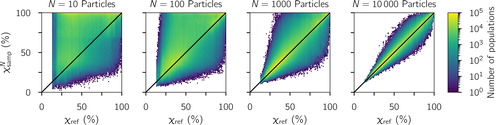
The sampling results are presented as two-dimensional histograms that, for each sample size N, include all 1000 samples of the 24,000 simulated reference populations (resulting in 24,000,000 data points for each sample size). Figure 2 shows ${\chi }_{\text{samp}}^N$ versus χ_ref for the four sample sizes. Estimating χ_ref based on a particle sample of only 10 particles led to results that can greatly overestimate or underestimate χ_ref. As the sample size increased from 10 to 10,000 particles the points converged on the one-to-one line, meaning that sampled mixing-state values more accurately approximate the associated reference values.

Figure 2. Distribution of sampled population mixing-state index ${\chi }_{\text{samp}}^N$ and reference mixing-state index χ_ref for increasing sample sizes based on the simulated scenario library described in Section 2.3. The solid black line is the 1:1 line.

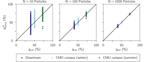
Figure 3 shows the corresponding plot using the field data from Pittsburgh. Each vertical cluster of points corresponds to data from a location or time period where the sampling occurred. Each of these clusters has a different χ_ref value, calculated from the full samples discussed in Section 2.4. For the downtown location, the χ_ref value was lowest (40%), consistent with the expectation for an area where fresh emissions mix with more aged aerosol. The aerosol at the CMU campus during winter (${\chi }_{\text{ref}}=51$%) was more externally mixed compared to the summer period (${\chi }_{\text{ref}}=72$%). This can be explained by the more extensive photochemical oxidation that drives the production of condensible secondary components, which condense onto preexisting particles and thus homogenize aerosol composition. A more detailed discussion on the spatial and temporal variability of aerosol mixing state in the Pittsburgh area can be found in Ye et al. (2018). Similar to the procedure used to analyze the modeled results, each χ_ref population was stochastically sub-sampled, which resulted in a range of ${\chi }_{\text{samp}}^N$ values that converged to the reference value as N increased.

Figure 3. Sampled ${\chi }_{\text{samp}}^N$ as a function of χ_ref from data obtained in Pittsburgh, PA. The one-to-one line is drawn for reference.

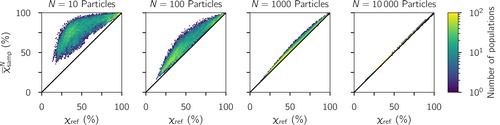
Both the simulation (Figure 2) and field data (Figure 3) results show that the sampled ${\chi }_{\text{samp}}^N$ has a positive bias. That is, it tends to be larger than the reference χ_ref. To investigate this more precisely, we computed the average ${\overline{\chi }}_{\text{samp}}^N$ for the simulation data, where the average is taken over all 1000 repeats and is mass-weighted (see Section 4.2 for details). This quantity is plotted versus χ_ref in Figure 4. In contrast to Figure 2 which displayed all individual 1000 × 24,000 data points, Figure 4 shows the averages over the 1000 repeats. This lets us see the patterns more clearly and confirms that ${\chi }_{\text{samp}}^N$ is positively biased (above the one-to-one line). As expected, the bias vanished as the sample size increased from 10 to 10,000 particles. The question arises of how this bias can be explained. In particular, since χ is the affine ratio of the average particle species diversity D_α and the bulk diversity D_γ (Equation (1)(1) $$\chi =\frac{D_{\alpha }-1}{D_{\gamma }-1}.$$(1) ), we need to determine the effect of sub-sampling on estimating these quantities individually before calculating the ratio.

Figure 4. Distribution of average sampled ${\overline{\chi }}_{\text{samp}}^N$ (averaged over the 1000 repeats) and χ_ref for increasing sample sizes based on the simulated scenario library described in Section 2.3. The one-to-one line is drawn for reference.

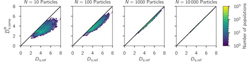
The positive bias is a result of biases in the average sampled diversity metrics, ${\overline{D}}_{\alpha ,\mathrm{s}\mathrm{amp}}^N$ and ${\overline{D}}_{\gamma ,\mathrm{s}\mathrm{amp}}^N.$ Figures 5 and 6 show the averaged sampled diversities versus reference diversities for the simulated populations. That is, Figure 5 shows the quantity needed for the numerator in Equation (1)(1) $$\chi =\frac{D_{\alpha }-1}{D_{\gamma }-1}.$$(1) , and Figure 6 shows the quantity needed for the denominator in Equation (1)(1) $$\chi =\frac{D_{\alpha }-1}{D_{\gamma }-1}.$$(1) . These show that, on average, sampling overestimates the mean particle diversity (D_α) and underestimates the total diversity (D_γ). Said another way, using a sample of particles will lead us to think that the average particle has more effective species than are really present, but that the bulk has less effective species than it actually does. Because χ is the affine ratio of mean particle to total diversity (see Equation (1)(1) $$\chi =\frac{D_{\alpha }-1}{D_{\gamma }-1}.$$(1) ), χ is thus overestimated. Writing these numerical observations in equations, we have (7) $${\overline{D}}_{\alpha ,\mathrm{s}\mathrm{amp}}^N\ge D_{\alpha ,\mathrm{r}\mathrm{e}\mathrm{f}},\left[\text{sampled populations}\mathit{overestimate}\text{mean particle diversity}\right]$$(7) (8) $${\overline{D}}_{\gamma ,\mathrm{s}\mathrm{amp}}^N\le D_{\gamma ,\mathrm{r}\mathrm{e}\mathrm{f}},\left[\text{sampled}\mathit{ }\text{populations}\mathit{underestimate}\text{total diversity}\right]$$(8) (9) $${\overline{\chi }}_{\text{samp}}^N\ge {\chi }_{\text{ref}}.[\text{sampled populations}\mathit{overestimate}\text{mixing}–\text{state index}]$$(9)

Figure 5. Distribution of average sampled ${\overline{D}}_{\alpha ,\mathrm{s}\mathrm{amp}}^N$ (mean particle diversity, averaged over the 1000 repeats) and $D_{\alpha ,\text{ref}}$ (reference mean particle diversity) for increasing sample sizes based on the simulated scenario library described in Section 2.3. The one-to-one line is drawn for reference.

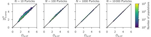
Figure 6. Distribution of average sampled ${\overline{D}}_{\gamma ,\mathrm{s}\mathrm{amp}}^N$ (total diversity, averaged over the 1000 repeats) and $D_{\gamma ,\text{ref}}$ (reference total diversity) for increasing sample sizes based on the simulated scenario library described in Section 2.3. The one-to-one line is drawn for reference.

Section 4 provides rigorous definitions of the sampling and averaging procedures and proves certain aspects of the above results.

To understand how many particles we should sample to be confident that the error is likely below some threshold, it is helpful to think about confidence intervals for the reference χ. The 95% confidence intervals for reference values, χ_ref, are shown in Figure 7 as a range Δχ about the sampled values ${\chi }_{\text{samp}}^N.$ This means that, if we measure a ${\chi }_{\text{samp}}^N$ value from a sampled particle population, 95% of the time the true χ_ref value will fall within the range ${\chi }_{\text{samp}}^N+\Delta \chi .$

Figure 7. 95%-Confidence intervals for sampled ${\chi }_{\text{samp}}^N$ values for sample sizes of N = 10, 100, 1000, and 10,000 particles based on the simulated scenario library described in Section 2.3.

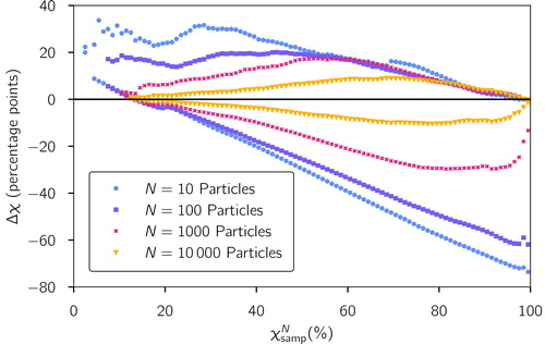
For small sample sizes N, the confidence interval is highly asymmetric and larger for populations that appear more internally mixed. For example, assuming that a sample of 10 particles is used to compute a sampled ${\chi }_{\text{samp}}^{10}$ value of 20%, the 95% confidence interval for the reference χ_ref for the whole population extends from 15% to 45% (i.e., Δχ ranges from −5 to + 25 percentage points). In contrast, for a ${\chi }_{\text{samp}}^{10}$ value of 90%, the confidence interval extends from 20% to 95% (Δχ from −70 to + 5 points).

For large sample sizes (e.g., N = 10,000), the confidence interval is narrow for large and small sampled χ values. It broadens for intermediate χ values, but remains within ±10 percentage points. It is reasonable that both highly diverse (low χ) and highly homogeneous (high χ) populations can have their mixing state measured well from a reasonably small sample. More complex distributions with intermediate χ require the sampling of more particles to obtain accurate estimates of the mixing state index.

By the central limit theorem, we expect that the sampling error should decrease proportionally to the square root of the number of particles. We can observe this in Figure 7, where going from N = 1000 to N = 10,000 particles reduced the 95% confidence interval bound by a factor of 3 (from 30 percentage points to 10 points), which is approximately $\sqrt{10},$ the square root of the increase in the number of samples.

Considering that the true χ value of a population is not known a priori, our results suggest that a sample size of 1000 particles is needed to obtain an estimate of χ within 30 percentage points and 10,000 particles are needed to determine χ within 10 percentage points for any mixing state.

4. Mathematical proofs

In Section 3 we have seen that ${\overline{\chi }}_{\text{samp}}^N$ is positively biased, which was caused by a positive bias in ${\overline{D}}_{\alpha ,\text{samp}}^N,$ a negative bias in ${\overline{D}}_{\gamma ,\text{samp}}^N,$ and the fact that $\chi =(D_{\alpha }-1)/(D_{\gamma }-1).$ In this section, we will show that the overestimation of D_α and underestimation of D_γ are both consequences of the entropy averaging procedures combined with convexity of the exponential function (for D_α) and concavity of the entropy function (for D_γ). To do this, we will start by precisely defining what we mean by sampling and averaging, and then we will prove the results themselves.

4.1. Notation for sampled particle populations

We consider a reference population of particles to be a set $\pi =\{{\overrightarrow{\mu }}_1,\dots ,{\overrightarrow{\mu }}_N\}.$ We use uppercase letters I, J to denote reference particle indices in π. Each particle is a vector ${\overrightarrow{\mu }}_I\in {\mathbb{R}}^A$ with coordinates ${\overrightarrow{\mu }}_I=({\mu }_I^1,\dots ,{\mu }_I^A),$ where each coordinate ${\mu }_I^a$ is the mass of species a in particle I. We use superscripts for species indexes and subscripts for particle indexes.

Consider sampled populations $\{{\pi }_1,\dots ,{\pi }_S\}$ from π. Each sampled population ${\pi }_s=\{{\overrightarrow{\mu }}_{s,1},\dots ,{\overrightarrow{\mu }}_{s,N_s}\}$ has N_s particles corresponding to reference particle indices $I_{s,1},\dots ,I_{s,N_s}.$ We use lowercase letters i, j for sampled particle indices and we write ${\overrightarrow{\mu }}_{s,i}$ for the i-th particle in sample s. The mass of species a in particle i of sample s is thus ${\mu }_{s,i}^a.$ The sampled particle ${\overrightarrow{\mu }}_{s,i}$ is equal to reference particle ${\overrightarrow{\mu }}_I$ with $I=I_{s,i},$ so the set of all reference particle indexes in a given sampled population is ${\mathcal{I}}_s=\left\{I_{s,i}\right|i=1,\dots ,N_s\}.$

Given a per-particle quantity X_I, we write $X_{s,i}=X_I$ when the reference index matches the sampled particle index: $I=I_{s,i}.$ To understand sampled diversities versus reference-population diversities, we want to compare mass-weighted averages computed over the reference population, and over sampled populations. To do this, we will now introduce the Iverson bracket and the key averaging lemma (Lemma 1).

The Iverson bracket gives a binary indicator of set membership: (10) $$[I\in {\mathcal{I}}^s]=\{\begin{array}{cc}1\hfill & \text{if}\mathit{ }I\in {\mathcal{I}}^s,\hfill \\ 0\hfill & \text{otherwise}.\hfill \end{array}$$(10)

Using the Iverson bracket we can translate between local and global indexes: (11) $$\sum _{i=1}^{N_s}{X}_{s,i}=\sum _{I=1}^N[I\in {\mathcal{I}}^s]X_I.$$(11)

In this article we consider particle populations to be sets, which means that all particles in the population must have at least one species with a different mass. In particular, this excludes monodisperse populations. To overcome this limitation we could consider populations to be multisets in the sense of (Knuth 1998, p. 473). Roughly speaking, a multiset is an extension of a set to allow elements to appear multiple times and for which the set union $\uplus$ and set union $\setminus$ operators have been appropriately extended. For multisets, the equivalent to the Iverson bracket is the multiplicity operator which gives the integer number of occurrences of any particle in the population. All the theoretical results in this article carry through for multisets, but we restrict ourselves to regular sets for convenience.

4.2. Mass fractions and mass-weighted probability distributions

Given a reference population $\pi =\{{\overrightarrow{\mu }}_1,\dots ,{\overrightarrow{\mu }}_N\}$ and sampled populations ${\pi }_s=\{{\overrightarrow{\mu }}_{s,1},\dots ,{\overrightarrow{\mu }}_{s,N_s}\}$ for $s=1,\dots ,S,$ as described in Section 4.1, we define the total masses: (12) $${\mu }_I=\sum _{a=1}^A{\mu }_I^a,\hspace{0.17em}\hspace{0.17em}\left[\text{total mass of reference particle}I\right]$$(12) (13) $${\mu }_{\text{tot}}=\sum _{I=1}^N{\mu }_I,\hspace{0.17em}\hspace{0.17em}\left[\text{total mass of reference population}\right]$$(13) (14) $${\mu }_{s,i}=\sum _{a=1}^A{\mu }_{s,i}^a,\hspace{0.17em}\hspace{0.17em}\left[\text{total mass of particle}i\text{in sampled population}s\right]$$(14) (15) $${\mu }_{s,\text{tot}}=\sum _{i=1}^{N_s}{\mu }_{s,i},\hspace{0.17em}\hspace{0.17em}\left[\text{total mass of sampled population}s\right]$$(15) (16) $${\mu }_{\text{samp},\text{tot}}=\sum _{s=1}^S{\mu }_{s,\text{tot}}.\hspace{0.17em}\hspace{0.17em}\left[\text{total mass of all}\text{sampled populations}\right]$$(16)

From this we define the mass fractions (or probabilities): (17) $$p_I=\frac{{\mu }_I}{{\mu }_{\text{tot}}},\hspace{0.17em}\hspace{0.17em}\left[\text{mass fraction of reference particle}I\right]$$(17) (18) $$p_{s,i}=\frac{{\mu }_{s,i}}{{\mu }_{s,\text{tot}}},\hspace{0.17em}\hspace{0.17em}\left[\text{mass fraction of particle}i\text{in sampled population}s\right]$$(18) (19) $$p_{s,\text{tot}}=\frac{{\mu }_{s,\text{tot}}}{{\mu }_{\text{samp},\text{tot}}}.\hspace{0.17em}\hspace{0.17em}\left[\text{mass fraction of sampled population}s\right]$$(19)

Interpreting these mass fractions as probabilities gives mass-weighted probability distributions over particle populations. For example, we can define the distribution $p_{\mathit{I}}$ to be the distribution over reference particles so that the probability $I\sim p_{\mathit{I}}$ of reference particle I is p_I. Doing this similarly for $p_{s,\mathit{i}}$ and $p_{\mathit{s},\text{tot}}$ gives us probability distributions over sampled particles and the set of sampled populations. Note that we are using roman-letter subscripts to denote probability distributions.

Consider a quantity X that can be indexed by either the reference particle index, X_I, the sampled particle indexes, $X_{s,i},$ or the sampled population index, $X_{s,\text{tot}}.$ Then we can compute expected values with respect to the mass-weighted probability distributions by averaging over the corresponding sets: (20) $${\mathbb{E}}_{I\sim p_{\mathit{I}}}\left[X_I\right]=\sum _{I=1}^N{p}_I{X}_I=\sum _{I=1}^N\frac{{\mu }_I}{{\mu }_{\text{tot}}}{X}_I,\hspace{0.17em}\hspace{0.17em}\left[\text{reference average}\right]$$(20) (21) $${\mathbb{E}}_{i\sim p_{s,\mathit{i}}}\left[X_{s,i}\right]=\sum _{i=1}^{N_s}{p}_{s,i}{X}_{s,i}=\sum _{i=1}^{N_s}\frac{{\mu }_{s,i}}{{\mu }_{s,\text{tot}}}{X}_{s,i},\hspace{0.17em}\hspace{0.17em}\left[\text{sample average}\right]$$(21) (22) $${\mathbb{E}}_{s\sim p_{\mathit{s},\text{tot}}}\left[X_{s,\text{tot}}\right]=\sum _{s=1}^S{p}_{s,\text{tot}}{X}_{s,\text{tot}}=\sum _{s=1}^S\frac{{\mu }_{s,\text{tot}}}{{\mu }_{\text{samp},\text{tot}}}{X}_{s,\text{tot}}.\hspace{0.17em}\hspace{0.17em}\left[\text{average over samples}\right]$$(22)

4.3. Entropy and diversity measures of mixing state

The entropy H associated with a vector $\overrightarrow{p}$ of mass fractions (equivalently, probabilities) is (23) $$H(\overrightarrow{p})=-\sum _{a=1}^A{p}^a\hspace{0.17em}\text{log}\hspace{0.17em}(p^a).$$(23)

The diversity D is the exponential of the entropy: (24) $$D(\overrightarrow{p})=\hspace{0.17em}\text{exp}\hspace{0.17em}(H(\overrightarrow{p})).$$(24)

Importantly, entropy is a concave function, which is fundamental to our results on over- and under-estimation of mixing-state measures. In fact, entropy is also log-concave in low dimensions (Alirezaei and Mathar 2018), which will be used in the proof of Theorem 4.

The mass fractions in a particle (equivalently, species probability vector) can be indexed by either reference or sampled particle indexes. These are thus: (25) $${\overrightarrow{p}}_I=\frac{{\overrightarrow{\mu }}_I}{{\mu }_I},\hspace{0.17em}\hspace{0.17em}\left[\text{species mass fractions in reference particle}I\right]$$(25) (26) $${\overrightarrow{p}}_{s,i}=\frac{{\overrightarrow{\mu }}_{s,i}}{{\mu }_{s,i}}.\hspace{0.17em}\hspace{0.17em}[\text{species mass fractions in particle}i\text{in sampled population}s]$$(26) Using the particle species mass fraction vectors, we denote the particle entropy by $H_I=H({\overrightarrow{p}}_I)$ with reference particle indexes and $H_{s,i}=H({\overrightarrow{p}}_{s,i})$ with sampled particle indexes. Similarly, we write D_I and $D_{s,i}$ for the corresponding diversities.

The α-entropy of a particle population is the mass-weighted average of the particle entropies, with the corresponding α-diversity. That is, α-entropies and α-diversities for our populations are (27) $$H_{\alpha ,\mathrm{r}\mathrm{e}\mathrm{f}}=\sum _{I=1}^N{p}_I{H}_I={\mathbb{E}}_{I\sim p_{\mathit{I}}}\left[H_I\right],\hspace{0.17em}\hspace{0.17em}[\alpha -\text{entropy of reference population}]$$(27) (28) $$H_{\alpha ,s}=\sum _{i=1}^{N_s}{p}_{s,i}{H}_{s,i}={\mathbb{E}}_{i\sim p_{s,\mathit{i}}}\left[H_{s,i}\right],\hspace{0.17em}\hspace{0.17em}\hspace{0.17em}\hspace{0.17em}[\alpha -\text{entropy of sampled population}s]$$(28) (29) $$D_{\alpha ,\mathrm{r}\mathrm{e}\mathrm{f}}=\hspace{0.17em}\text{exp}\hspace{0.17em}(H_{\alpha ,\mathrm{r}\mathrm{e}\mathrm{f}}),\hspace{0.17em}\hspace{0.17em}\hspace{0.17em}\hspace{0.17em}\hspace{0.17em}\hspace{0.17em}[\alpha -\text{diversity of reference population}]$$(29) (30) $$D_{\alpha ,s}=\hspace{0.17em}\text{exp}\hspace{0.17em}(H_{\alpha ,s}).\hspace{0.17em}\hspace{0.17em}\hspace{0.17em}\hspace{0.17em}\hspace{0.17em}\hspace{0.17em}\hspace{0.17em}\hspace{0.17em}[\alpha -\text{diversity of sampled population}s]$$(30)

The γ-entropy of a population is the entropy of the mass-weighted average composition vector, with the corresponding γ-diversity. That is, while α-entropy is the average of entropies, γ-entropy is the entropy of the average. This gives: (31) $$H_{\gamma ,\mathrm{r}\mathrm{e}\mathrm{f}}=H(\sum _{I=1}^N{p}_I{\overrightarrow{p}}_I)=H({\mathbb{E}}_{I\sim p_{\mathit{I}}}[{\overrightarrow{p}}_I]),\hspace{0.17em}\hspace{0.17em}\hspace{0.17em}\hspace{0.17em}[\gamma -\text{entropy of reference population}]$$(31) (32) $$H_{\gamma ,s}=H(\sum _{i=1}^{N_s}{p}_{s,i}{\overrightarrow{p}}_{s,i})=H({\mathbb{E}}_{i\sim p_{s,\mathit{i}}}[{\overrightarrow{p}}_{s,i}]),\hspace{0.17em}\hspace{0.17em}\hspace{0.17em}\hspace{0.17em}[\gamma -\text{entropy of sampled population}s]$$(32) (33) $$D_{\gamma ,\mathrm{r}\mathrm{e}\mathrm{f}}=\hspace{0.17em}\text{exp}\hspace{0.17em}(H_{\gamma ,\mathrm{r}\mathrm{e}\mathrm{f}}),\hspace{0.17em}\hspace{0.17em}[\gamma -\text{diversity of reference population}]$$(33) (34) $$D_{\gamma ,s}=\hspace{0.17em}\text{exp}\hspace{0.17em}(H_{\gamma ,s}).\hspace{0.17em}\hspace{0.17em}\hspace{0.17em}\hspace{0.17em}[\gamma -\text{diversity of sampled population}s]$$(34)

From the population diversities we define the overall mixing-state index of a population to be the affine ratio: (35) $${\chi }_{\text{ref}}=\frac{D_{\alpha ,\mathrm{r}\mathrm{e}\mathrm{f}}-1}{D_{\gamma ,\mathrm{r}\mathrm{e}\mathrm{f}}-1},\hspace{0.17em}\hspace{0.17em}\hspace{0.17em}\hspace{0.17em}\hspace{0.17em}\hspace{0.17em}[\text{mixing}-\text{state index of reference}\text{population}]$$(35) (36) $${\chi }_s=\frac{D_{\alpha ,s}-1}{D_{\gamma ,s}-1}.\hspace{0.17em}\hspace{0.17em}\hspace{0.17em}\hspace{0.17em}\hspace{0.17em}\hspace{0.17em}[\text{mixing}-\text{state index of sampled}\text{population}s]$$(36)

We are particularly interested in the average sampled entropies and diversities, where the mass-weighted average is taken over all sampled populations. This gives (37) $${\overline{H}}_{\alpha ,\mathrm{s}\mathrm{amp}}=E_{s\sim p_{\mathit{s}}}\left[H_{\alpha ,s}\right],\hspace{0.17em}\hspace{0.17em}\hspace{0.17em}\hspace{0.17em}[\text{average sampled}\alpha -\text{entropy}]$$(37) (38) $${\overline{H}}_{\gamma ,\mathrm{s}\mathrm{amp}}=E_{s\sim p_{\mathit{s}}}\left[H_{\gamma ,s}\right],\hspace{0.17em}\hspace{0.17em}\hspace{0.17em}\hspace{0.17em}[\text{average sampled}\gamma -\text{entropy}]$$(38) (39) $${\overline{D}}_{\alpha ,\mathrm{s}\mathrm{amp}}=E_{s\sim p_{\mathit{s}}}\left[D_{\alpha ,s}\right],\hspace{0.17em}\hspace{0.17em}\hspace{0.17em}\hspace{0.17em}[\text{average sampled}\alpha -\text{diversity}]$$(39) (40) $${\overline{D}}_{\gamma ,\mathrm{s}\mathrm{amp}}=E_{s\sim p_{\mathit{s}}}\left[D_{\gamma ,s}\right],\hspace{0.17em}\hspace{0.17em}\hspace{0.17em}\hspace{0.17em}[\text{average sampled}\gamma -\text{diversity}]$$(40) (41) $${\overline{\chi }}_{\text{samp}}=E_{s\sim p_{\mathit{s}}}\left[{\chi }_s\right].\hspace{0.17em}\hspace{0.17em}\hspace{0.17em}\hspace{0.17em}[\text{average sampled mixing}-\text{state index}]$$(41)

4.4. Fair sampling and a fundamental lemma

The sampled populations may all contain the same number of particles, in which case N_s is independent of s, or they may be of different sizes. Our theoretical results apply in either case, so long as we assume that the sampled populations sample all particles fairly. To make this precise, we define N_I to be the number of sampled populations containing particle I: (42) $$N_I=\sum _{s=1}^S[I\in {\mathcal{I}}_s].$$(42)

Using this, we make our assumption precise as follows.

Assumption 1 (Uniform sampling). Each particle in the population appears in the same number of sampled populations, so N_I = N_J for any $I,J=1,\dots ,N.$

Lemma 1.

Given a per-particle quantity X indexed both by the reference index, X_I, and sampled population indexes, $X_{s,i}$, the mass-weighted average of X over all particles in all sampled populations is the same as the mass-weighted average over all reference particles: (43) $${\mathbb{E}}_{s\sim p_{\mathit{s},\text{tot}}}[\underset{X_{s,\text{tot}}}{\underbrace{{\mathbb{E}}_{i\sim p_{s,\mathit{i}}}[X_{s,i}]}}]={\mathbb{E}}_{I\sim p_{\mathit{I}}}\left[X_I\right].$$(43)

Proof.

Starting from the left hand side (LHS) of (43), we compute: (44) $$\text{LHS}=\sum _{s=1}^S\frac{{\mu }_{s,\text{tot}}}{{\mu }_{\text{samp},\text{tot}}}\sum _{i=1}^{N_s}\frac{{\mu }_{s,i}}{{\mu }_{s,\text{tot}}}{X}_{s,i}\hspace{0.17em}\hspace{0.17em}[\text{Equations} (21)\text{and} (22)]$$(44) (45) $$=\frac{1}{{\mu }_{\text{samp},\text{tot}}}\sum _{s=1}^S\sum _{i=1}^{N_s}{\mu }_{s,i}{X}_{s,i}$$(45) (46) $$=\frac{1}{\sum _{s=1}^S\sum _{i=1}^{N_s}{\mu }_{s,i}}\sum _{s=1}^S\sum _{i=1}^{N_s}{\mu }_{s,i}{X}_{s,i}[\text{Equations} (15)\text{and} (16)]$$(46) (47) $$=\frac{1}{\sum _{s=1}^S\sum _{J=1}^N[J\in {\mathcal{I}}_s]{\mu }_J}\sum _{s=1}^S\sum _{I=1}^N[I\in {\mathcal{I}}_s]{\mu }_I{X}_I\mathit{ }[\text{Equation} (11)]$$(47) (48) $$=\frac{1}{\sum _{J=1}^N{\mu }_J\sum _{s=1}^S[J\in {\mathcal{I}}_s]}\sum _{I=1}^N{\mu }_I{X}_I\sum _{s=1}^S[I\in {\mathcal{I}}_s]$$(48) (49) $$=\frac{1}{\sum _{J=1}^N{\mu }_J{N}_J}\sum _{I=1}^N{\mu }_I{X}_I{N}_I[\text{Equation} (42)]$$(49) (50) $$=\frac{1}{\sum _{J=1}^N{\mu }_J}\sum _{I=1}^N{\mu }_I{X}_I[\text{Assumption} 1]$$(50) (51) $$={\mathbb{E}}_{I\sim p_{\mathit{I}}}\left[X_I\right].[\text{Equations} (13)\text{and} (20)]$$(51)

4.5. Theoretical sampling results for mixing-state measures

We are now ready to prove our main results, which describe how the average sampled entropies and diversities relate to the reference entropies and diversities. To summarize, we will show that (52) $${\overline{H}}_{\alpha ,\mathrm{s}\mathrm{amp}}=H_{\alpha ,\mathrm{r}\mathrm{e}\mathrm{f}},\hspace{0.17em}\hspace{0.17em}[\text{exactly estimate}\alpha -\text{entropy from samples}]$$(52) (53) $${\overline{H}}_{\gamma ,\mathrm{s}\mathrm{amp}}\le H_{\gamma ,\mathrm{r}\mathrm{e}\mathrm{f}},\hspace{0.17em}\hspace{0.17em}[\text{underestimate}\gamma -\text{entropy from samples}]$$(53) (54) $${\overline{D}}_{\alpha ,\mathrm{s}\mathrm{amp}}\ge D_{\alpha ,\mathrm{r}\mathrm{e}\mathrm{f}},\hspace{0.17em}\hspace{0.17em}[\text{overestimate}\alpha -\text{diversity from samples}]$$(54) (55) $${\overline{D}}_{\gamma ,\mathrm{s}\mathrm{amp}}\le D_{\gamma ,\mathrm{r}\mathrm{e}\mathrm{f}}.\hspace{0.17em}\hspace{0.17em}[\text{underestimate}\gamma -\text{diversity fromsamples}(\text{only with}2\text{or}3\text{species})]$$(55)

See Figures 5 and 6 for numerical simulations that confirm (54) and (55), respectively.

The mixing-state index χ is the affine ratio of D_α to D_γ, so overestimating D_α and underestimating D_γ makes it plausible that the average sampled ${\overline{\chi }}_{\text{samp}}$ values will overestimate the reference χ_ref. As shown in Figure 4, numerical simulations on atmospherically relevant particle populations show that ${\overline{\chi }}_{\text{samp}}$ values do indeed overestimate χ_ref. However, because $D_{\alpha ,s}$ is correlated with $D_{\gamma ,s},$ it is not straightforward to prove a precise relationship between ${\overline{\chi }}_{\text{samp}}$ and χ_ref.

In all of the following results we are using mass-weighted averages, as defined in Section 4.2, which is natural because α- and γ-entropy are mass-weighted quantities. We begin by showing that mass-weighted averaging results in reference and sampled α-diversities being equal on average.

Theorem 1

(Sampled α-entropy). If the sampled populations are drawn uniformly from the reference population (Assumption 1) then the average sampled α-entropy is equal to the reference α-entropy: (56) $${\overline{H}}_{\alpha ,\mathrm{s}\mathrm{amp}}=H_{\alpha ,\mathrm{r}\mathrm{e}\mathrm{f}}.$$(56)

Proof.

We compute (57) $${\overline{H}}_{\alpha ,\mathrm{s}\mathrm{amp}}=E_{s\sim p_{\mathit{s}}}\left[H_{\alpha ,s}\right]\hspace{0.17em}\hspace{0.17em}\left[\text{Definition}\mathit{ }\text{of}\mathit{ }{\overline{H}}_{\alpha ,\mathrm{s}\mathrm{amp}}\right]$$(57) (58) $$=E_{s\sim p_{\mathit{s}}}\left[E_{i\sim p_{s,\mathit{i}}}\right[H({\overrightarrow{p}}_{s,i})\left]\right]\hspace{0.17em}\hspace{0.17em}\left[\text{Definition}\mathit{ }\text{of}\mathit{ }{H}_{\alpha ,s}\right]$$(58) (59) $$=E_{I\sim p_{\mathit{I}}}[H({\overrightarrow{p}}_I)]\hspace{0.17em}\hspace{0.17em}[\text{Lemma} 1]$$(59) (60) $$=H_{\alpha ,\mathrm{r}\mathrm{e}\mathrm{f}}.\hspace{0.17em}\hspace{0.17em}\hspace{0.17em}\hspace{0.17em}\left[\text{Definition}\mathit{ }\text{of}\mathit{ }{H}_{\alpha ,\mathrm{r}\mathrm{e}\mathrm{f}}\right]$$(60) □

Next, we show that concavity of entropy means that γ-entropy is consistently underestimated from sampled populations.

Theorem 2

(Sampled γ-entropy). If the sampled populations are drawn uniformly from the reference population (Assumption 1) then the average sampled γ-entropy is less than or equal to the reference γ-entropy: (61) $${\overline{H}}_{\gamma ,\mathrm{s}\mathrm{amp}}\le H_{\gamma ,\mathrm{r}\mathrm{e}\mathrm{f}}.$$(61)

Proof.

Similarly to Theorem 1, but with expectations and entropy reversed, we compute (62) $${\overline{H}}_{\gamma ,\mathrm{s}\mathrm{amp}}=E_{s\sim p_{\mathit{s}}}\left[H_{\gamma ,s}\right]\hspace{0.17em}\hspace{0.17em}\left[\text{Definition}\mathit{ }\text{of}\mathit{ }{\overline{H}}_{\gamma ,\mathrm{s}\mathrm{amp}}\right]$$(62) (63) $$=E_{s\sim p_{\mathit{s}}}[H(E_{i\sim p_{s,\mathit{i}}}\left[{\overrightarrow{p}}_{s,i}\right])]\hspace{0.17em}\hspace{0.17em}\left[\text{Definition}\mathit{ }\text{of}\mathit{ }{H}_{\gamma ,s}\right]$$(63) (64) $$\le H(E_{s\sim p_{\mathit{s}}}[E_{i\sim p_{s,\mathit{i}}}\left[{\overrightarrow{p}}_{s,i}\right]])[\text{Jensen}\text{'}\text{s inequality and concavity of}H]$$(64) (65) $$=H(E_{I\sim p_{\mathit{I}}}[{\overrightarrow{p}}_I])\hspace{0.17em}\hspace{0.17em}\hspace{0.17em}\hspace{0.17em}[\text{Lemma} 1]$$(65) (66) $$=H_{\gamma ,\mathrm{r}\mathrm{e}\mathrm{f}}.\hspace{0.17em}\hspace{0.17em}\hspace{0.17em}\hspace{0.17em}\left[\text{Definition}\mathit{ }\text{of}\mathit{ }{H}_{\gamma ,\mathrm{r}\mathrm{e}\mathrm{f}}\right]$$(66) □

Having established the average behavior of sampled entropies, we now turn our attention to sampled diversities. We begin by showing that the α-diversity is consistently overestimated from sampled populations, as we saw in Figure 5. The reason for this overestimation is that the exponential function is convex, as illustrated in Figure 8.

Figure 8. Schematic to illustrate Theorem 3. Here we consider two sampled populations with α-diversities of $H_{\alpha ,1}$ and $H_{\alpha ,2},$ which we assume have average exactly equal to the reference value $H_{\alpha ,\mathrm{r}\mathrm{e}\mathrm{f}}$ (this is true on average, as we saw from Theorem 1). The exponential function maps entropies H to diversities D, and because it is convex the average sampled value, ${\overline{D}}_{\alpha ,\mathrm{s}\mathrm{amp}},$ will be greater than the reference value, $D_{\alpha ,\mathrm{r}\mathrm{e}\mathrm{f}}.$

Theorem 3

(Sampled α-diversity). If the sampled populations are drawn uniformly from the reference population (Assumption 1) then the average sampled α-diversity is greater than or equal to the reference α-diversity: (67) $${\overline{D}}_{\alpha ,\mathrm{s}\mathrm{amp}}\ge D_{\alpha ,\mathrm{r}\mathrm{e}\mathrm{f}}.$$(67)

Proof.

Using Theorem 1 gives (68) $${\overline{D}}_{\alpha ,\mathrm{s}\mathrm{amp}}=E_{s\sim p_{\mathit{s}}}\left[D_{\alpha ,s}\right]\hspace{0.17em}\hspace{0.17em}\hspace{0.17em}\hspace{0.17em}\left[\text{Definition}\mathit{ }\text{of}\mathit{ }{\overline{D}}_{\alpha ,\mathrm{s}\mathrm{amp}}\right]$$(68) (69) $$=E_{s\sim p_{\mathit{s}}}[\text{exp}\hspace{0.17em}(H_{\alpha ,s})]\hspace{0.17em}\hspace{0.17em}\hspace{0.17em}\hspace{0.17em}\left[\text{Diversity}\mathit{ }\text{is}\mathit{ }\text{the}\mathit{ }\text{exponential}\mathit{ }\text{of}\mathit{ }\text{entropy}\right]$$(69) (70) $$\ge \hspace{0.17em}\text{exp}\hspace{0.17em}(E_{s\sim p_{\mathit{s}}}[H_{\alpha ,s}])\hspace{0.17em}\hspace{0.17em}[\text{Jensen}\text{'}\text{s inequality and}\text{convexity of exp}]$$(70) (71) $$=\hspace{0.17em}\text{exp}\hspace{0.17em}(H_{\alpha ,\mathrm{r}\mathrm{e}\mathrm{f}})\hspace{0.17em}\hspace{0.17em}\hspace{0.17em}\hspace{0.17em}[\text{Theorem} 1]$$(71) (72) $$=D_{\alpha ,\mathrm{r}\mathrm{e}\mathrm{f}}.\hspace{0.17em}\hspace{0.17em}\left[\text{Diversity is the exponential of entropy}\right]$$(72) □

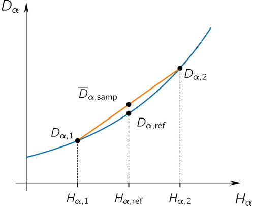
Finally, we consider the sampled γ-diversity. Because entropy is only log-concave in dimensions 2 and 3, we are only able to prove a consistent relationship when we have these number of species. As shown in Figure 6, however, even in higher dimensions we see from numerical simulations that sampled populations tend to underestimate D_γ. Figure 9 illustrates how concavity of the diversity function leads to underestimation.

Figure 9. Schematic to illustrate Theorem 4 in the case of a two-species aerosol population, where p is the mass fraction of the first species. We consider two sampled populations with first-species mass-fractions of p₁ and p₂, which we assume have average exactly equal to the first-species reference mass fraction of p_ref (this is exactly true on average by (43(43) $${\mathbb{E}}_{s\sim p_{\mathit{s},\text{tot}}}[\underset{X_{s,\text{tot}}}{\underbrace{{\mathbb{E}}_{i\sim p_{s,\mathit{i}}}[X_{s,i}]}}]={\mathbb{E}}_{I\sim p_{\mathit{I}}}\left[X_I\right].$$(43) )). The diversity function is concave (for 2 or 3 species) so the average sampled value, ${\overline{D}}_{\gamma ,\mathrm{s}\mathrm{amp}},$ will be less than the reference value, $D_{\gamma ,\mathrm{r}\mathrm{e}\mathrm{f}}.$

Theorem 4

(Sampled γ-diversity). If the sampled populations are drawn uniformly from the reference population (Assumption 1) and the number of species is 2 or 3, then the average sampled γ-diversity is less than or equal to the reference γ-diversity: (73) $${\overline{D}}_{\gamma ,\mathrm{s}\mathrm{amp}}\le D_{\gamma ,\mathrm{r}\mathrm{e}\mathrm{f}}.$$(73)

Proof.

This proof is almost identical to that of Theorem 2, except we use the fact that D is concave in dimension 2 or 3. Because $D(·)=\hspace{0.17em}\text{exp}\hspace{0.17em}(H(·)),$ or equivalently $H(·)=\hspace{0.17em}\text{log}\hspace{0.17em}(D(·)),$ concavity of D is equivalent to log-concavity of H. As shown in Alirezaei and Mathar (2018, Theorem 16), H is log-concave if and only if the dimension (number of species) is 2 or 3.

Assuming we have 2 or 3 species and thus concave D, we compute (74) $${\overline{D}}_{\gamma ,\mathrm{s}\mathrm{amp}}=E_{s\sim p_{\mathit{s}}}\left[D_{\gamma ,s}\right]\hspace{0.17em}\hspace{0.17em}\left[\text{Definition}\mathit{ }\text{of}\mathit{ }{\overline{D}}_{\gamma ,\mathrm{s}\mathrm{amp}}\right]$$(74) (75) $$=E_{s\sim p_{\mathit{s}}}[D(E_{i\sim p_{s,\mathit{i}}}\left[{\overrightarrow{p}}_{s,i}\right])]\hspace{0.17em}\hspace{0.17em}\left[\text{Definition}\mathit{ }\text{of}\mathit{ }{D}_{\gamma ,s}\right]$$(75) (76) $$\le D(E_{s\sim p_{\mathit{s}}}[E_{i\sim p_{s,\mathit{i}}}\left[{\overrightarrow{p}}_{s,i}\right]])\hspace{0.17em}\hspace{0.17em}[\text{Jensen}\text{'}\text{s inequality}\text{and concavity of}D]$$(76) (77) $$=D(E_{I\sim p_{\mathit{I}}}[{\overrightarrow{p}}_I])\hspace{0.17em}\hspace{0.17em}[\text{Lemma} 1]$$(77) (78) $$=D_{\gamma ,\mathrm{r}\mathrm{e}\mathrm{f}}.\hspace{0.17em}\hspace{0.17em}\left[\text{Definition}\mathit{ }\text{of}\mathit{ }{D}_{\gamma ,\mathrm{r}\mathrm{e}\mathrm{f}}\right]$$(78) □

As we see from the above proofs, we now understand the source of the over/under-estimation of the average sampled mixing state index and diversity metrics that we observed from simulations and experimental data in Section 3. The consistent overestimation of D_α is a consequence of the exact averaging of H_α (Theorem 1) combined with the convexity of the exponential function (Theorem 3). The underestimation of D_γ (and H_γ), on the other hand, is due to the concavity of the (log-)entropy function (Theorems 2 and 4). By the central limit theorem, all of these over/under-estimations will decrease at a rate of $1/\sqrt{N}$ as the number of sampled particles, N, increases.

5. Conclusions

Single-particle instruments necessarily use finite particle samples to determine population-level quantities, with the sample size being determined by practical considerations of data acquisition. In this study we developed a method to determine confidence intervals for a population-level quantity, the mixing-state index χ, that is determined from particle-level information. We accomplished this by using model-generated particle populations as a reference, which were subsequentially subsampled. Both numerical and mathematical analyses revealed that finite particle samples introduce a positive bias in the estimation of the diversity metric D_α (the average particle species diversity), and a negative bias in D_γ (the bulk diversity), which overall results in a positive bias in the estimation of χ. These results are consistent with the measurements using the aerosol samples of the Ye et al. (2018) study of Pittsburgh. The confidence interval for χ, not surprisingly, depends on the mixing state itself.

A sample size of 1000 particles allows an estimate of χ within 30 percentage points, and 10,000 particles are needed to determine χ within 10 percentage points, for any mixing state. This approach could be extended to the measurement of other population-level quantities that are estimated based on particle samples. Furthermore, it may be important in practice to consider measurement error (not just undersampling) when calculating χ, or to extend χ to include species similarity (Leinster and Cobbold 2012) or functional diversity (Scheiner et al. 2017).

Data availability

The output of the particle-resolved modeling scenario library can be accessed at https://doi.org/10.13012/B2IDB-2774261_V1.

Additional information

Funding

We acknowledge funding from NSF AGS-1254428, NSF AGS-1543786, NSF CHE-1807530, and DOE ASR DE-SC0019192. This publication was developed under assistance agreement RD83587301 awarded by the U.S. Environmental Protection Agency as part of the Center for Air, Climate, and Energy Solutions. It has not been formally reviewed by EPA. The views expressed in this document are solely those of authors and do not necessarily reflect those of the Agency. EPA does not endorse any products or commercial services mentioned in this publication. This research is part of the Blue Waters sustained petascale computing project, which is supported by the National Science Foundation (awards OCI-0725070 and ACI-1238993) and the state of Illinois. Blue Waters is a joint effort of the University of Illinois at Urbana-Champaign and its National Center for Supercomputing Applications.

References

- Alirezaei, G., and R. Mathar. 2018. On exponentially concave functions and their impact in information theory. In Proceedings of the 2018 Information Theory and Applications Workshop (ITA). doi:10.1109/ITA.2018.8503202.
- Beck, J., and W. Schwanghart. 2010. Comparing measures of species diversity from incomplete inventories: An update. Methods Ecol. Evol. 1 (1):38–44. 00003.x. doi:10.1111/j.2041-210X.2009.
- Beck, J., J. D. Holloway, and W. Schwanghart. 2013. Undersampling and the measurement of beta diversity. Methods Ecol. Evol. 4 (4):370–82. doi:10.1111/2041-210x.12023.
- Beydoun, H., M. Polen, and R. C. Sullivan. 2017. A new multicomponent heterogeneous ice nucleation model and its application to snomax bacterial particles and a snomax–illite mineral particle mixture. Atmos. Chem. Phys. 17 (22):13545–57. doi:10.5194/acp-17-13545-2017.
- Bondy, A. L., D. Bonanno, R. C. Moffet, B. Wang, A. Laskin, and A. P. Ault. 2018. The diverse chemical mixing state of aerosol particles in the southeastern United States. Atmos. Chem. Phys. 18 (16):12595–612. doi:10.5194/acp-18-12595-2018.
- Brocklehurst, N., M. O. Day, and J. Fröbisch. 2018. Accounting for differences in species frequency distributions when calculating beta diversity in the fossil record. Methods Ecol. Evol. 9 (6):1409–20. doi:10.1111/2041-210X.13007.
- Butturi-Gomes, D., M. Petrere, H. C. Giacomini, and S. S. Zocchi. 2017. Statistical performance of a multicomparison method for generalized species diversity indices under realistic empirical scenarios. Ecol. Indic. 72:545–52. doi:10.1016/j.ecolind.2016.08.054.
- Chao, A., and L. Jost. 2015. Estimating diversity and entropy profiles via discovery rates of new species. Methods Ecol. Evol. 6 (8):873–82. doi:10.1111/2041-210X.12349.
- Chao, A., Y. T. Wang, and L. Jost. 2013. Entropy and the species accumulation curve: A novel entropy estimator via discovery rates of new species. Methods Ecol. Evol. 4 (11):1091–100. doi:10.1111/2041-210X.12108.
- Ching, J., J. Fast, M. West, and N. Riemer. 2017. Metrics to quantify the importance of mixing state for CCN activity. Atmos. Chem. Phys. 17 (12):7445–58. doi:10.5194/acp-17-7445-2017.
- Ching, J., N. Riemer, and M. West. 2016. Black carbon mixing state impacts on cloud microphysical properties: Effects of aerosol plume and environmental conditions. J. Geophys. Res. Atmos. 121 (10):5990–6013. doi:10.1002/2016JD024851.
- Daly, A. J., J. M. Baetens, and B. D. Baets. 2018. Ecological diversity: Measuring the unmeasurable. Mathematics 6 (7):119. doi:10.3390/math6070.
- Dickau, M., J. Olfert, M. E. J. Stettler, A. Boies, A. Momenimovahed, K. Thomson, G. Smallwood, and M. Johnson. 2016. Methodology for quantifying the volatile mixing state of an aerosol. Aerosol. Sci. Technol. 50 (8):759–72. doi:10.1080/02786826.2016.1185509.
- Fraund, M., D. Q. Pham, D. Bonanno, T. H. Harder, B. Wang, J. Brito, S. S. De Sá, S. Carbone, S. China, P. Artaxo, et al. 2017. Elemental mixing state of aerosol particles collected in Central Amazonia during GoAmazon2014/15. Atmosphere 8 (12):173. doi:10.3390/atmos8090173.
- Gasparik, J. T., Q. Ye, J. H. Curtis, A. A. Presto, N. M. Donahue, R. C. Sullivan, M. West, and N. Riemer. 2020. Data from: Quantifying errors in the aerosol mixing-state index based on limited particle sample size [dataset]. University of Illinois at Urbana-Champaign. doi:10.13012/B2IDB-2774261_V1.
- Haegeman, B., J. Hamelin, J. Moriarty, P. Neal, J. Dushoff, and J. S. Weitz. 2013. Robust estimation of microbial diversity in theory and in practice. ISME J. 7 (6):1092–101. doi:10.1038/ismej.2013.10.
- Healy, R. M., N. Riemer, J. C. Wenger, M. Murphy, M. West, L. Poulain, A. Wiedensohler, I. P. O'Connor, E. McGillicuddy, J. R. Sodeau, et al. 2014. Single particle diversity and mixing state measurements. Atmos. Chem. Phys. 14 (12):6289–99., doi:10.5194/acp-14-6289-2014.
- Healy, R., J. Sciare, L. Poulain, M. Crippa, A. Wiedensohler, A. Prévôt, U. Baltensperger, R. Sarda-Estève, M. McGuire, C.-H. Jeong, et al. 2013. Quantitative determination of carbonaceous particle mixing state in Paris using single-particle mass spectrometer and aerosol mass spectrometer measurements. Atmos. Chem. Phys. 13 (18):9479–96. doi:10.5194/acp-13-9479-2013.
- Hughes, M., J. K. Kodros, J. R. Pierce, M. West, and N. Riemer. 2018. Machine learning to predict the global distribution of aerosol mixing state metrics. Atmosphere 9 (1):15. doi:10.3390/atmos9010015.
- Knopf, D. A., and P. A. Alpert. 2013. A water activity based model of heterogeneous ice nucleation kinetics for freezing of water and aqueous solution droplets. Faraday Discuss. 165:513–34. doi:10.1039/c3fd00035d.
- Knuth, D. E. 1998. The art of computer programming, volume 2: Seminumerical Algorithms. 3rd ed. Boston, MA: Addison Wesley.
- Leinster, T., and C. A. Cobbold. 2012. Measuring diversity: The importance of species similarity. Ecology 93 (3):477–89. doi:10.1890/10-2402.1.
- Lesins, G., P. Chylek, and U. Lohmann. 2002. A study of internal and external mixing scenarios and its effect on aerosol optical properties and direct radiative forcing. J. Geophys. Res. 107 (D10):AAC 5-1–4106. doi:10.1029/2001JD000973.
- Marion, Z. H. 2016. On the quantification of complexity and diversity from phenotypes to ecosystems. Ph.D. thesis., University of Tennessee.
- Marion, Z. H., J. A. Fordyce, and B. M. Fitzpatrick. 2018. A hierarchical Bayesian model to incorporate uncertainty into methods for diversity partitioning. Ecology 99 (4):947–56. doi:10.1002/ecy.2174.
- Moffet, R. C., and K. A. Prather. 2009. In-situ measurements of the mixing state and optical properties of soot with implications for radiative forcing estimates. Proc. Natl. Acad. Sci. USA. 106 (29):11872–7. doi:10.1073/pnas.0900040106.
- O'Brien, R. E., B. Wang, A. Laskin, N. Riemer, M. West, Q. Zhang, Y. Sun, X. ‐Y. Yu, P. Alpert, D. A. Knopf, et al. 2015. Chemical imaging of ambient aerosol particles: Observational constraints on mixing state parameterization. J. Geophys. Res. Atmos. 120 (18):9591–605. doi:10.1002/2015JD023480.
- Prather, K. A., C. D. Hatch, and V. H. Grassian. 2008. Analysis of atmospheric aerosols. Annu Rev Anal Chem (Palo Alto Calif) 1:485–514. doi:10.1146/annurev.anchem.1.031207.113030.
- Riemer, N., A. Ault, M. West, R. Craig, and J. Curtis. 2019. Aerosol mixing state: Measurements, modeling, and impacts. Rev. Geophys. 57 (2):187–249. doi:10.1029/2018RG000615.
- Riemer, N., and M. West. 2013. Quantifying aerosol mixing state with entropy and diversity measurements. Atmos. Chem. Phys. 13 (22):11423–39. doi:10.5194/acp-13-11423-2013.
- Riemer, N., M. West, R. Zaveri, and R. Easter. 2009. Simulating the evolution of soot mixing state with a particle-resolved aerosol model. J. Geophys. Res 114 (D9):D09202. doi:10.1029/2008JD011073.
- Ryder, O. S., A. P. Ault, J. F. Cahill, T. L. Guasco, T. P. Riedel, L. A. Cuadra-Rodriguez, C. J. Gaston, E. Fitzgerald, C. Lee, K. A. Prather, et al. 2014. On the role of particle inorganic mixing state in the reactive uptake of N2O5 to ambient aerosol particles. Environ. Sci. Technol. 48 (3):1618–27. doi:10.1021/es4042622.
- Scheiner, S. M., E. Kosman, S. J. Presley, and M. R. Willig. 2017. Decomposing functional diversity. Methods Ecol. Evol. 8 (7):809–20. doi:10.1111/2041-210X.12696.
- Schell, B., I. J. Ackermann, H. Hass, F. S. Binkowski, and A. Ebel. 2001. Modeling the formation of secondary organic aerosol within a comprehensive air quality modeling system. J. Geophys. Res. 106 (D22):28275–93. doi:10.1029/2001JD000384.
- Sherwin, W. B., and N. Prat I Fornells. 2019. The introduction of entropy and information methods to ecology by Ramon Margalef. Entropy 21 (8):794. doi:10.3390/e21080794.
- Sullivan, R., M. Moore, M. Petters, S. Kreidenweis, G. Roberts, and K. Prather. 2009. Effect of chemical mixing state on the hygroscopicity and cloud nucleation properties of calcium mineral dust particles. Atmos. Chem. Phys. 9 (10):3303–16. doi:10.5194/acp-9-3303-2009.
- Winkler, P. 1973. The growth of atmospheric aerosol particles as a function of the relative humidity-II. An improved concept of mixed nuclei. J. Aerosol Sci. 4 (5):373–87. doi:10.1016/0021-8502(73)90027-X.
- Ye, Q., P. Gu, H. Z. Li, E. S. Robinson, E. Lipsky, C. Kaltsonoudis, A. K. Y. Lee, J. S. Apte, A. L. Robinson, R. C. Sullivan, et al. 2018. Spatial variability of sources and mixing state of atmospheric particles in a metropolitan area. Environ. Sci. Technol. 52 (12):6807–15., doi:10.1021/acs.est8b01011.
- Zaveri, R., and L. Peters. 1999. A new lumped structure photochemical mechanism for large-scale applications. J. Geophys. Res. 104 (D23):30387–415. doi:10.1029/1999JD900876.
- Zaveri, R., R. Easter, and A. Wexler. 2005b. A new method for multicomponent activity coefficients of electrolytes in aqueous atmospheric aerosols. J. Geophys. Res. 110 (D2), D02201. doi:10.1029/2004JD004681.
- Zaveri, R., R. Easter, and L. Peters. 2005a. A computationally efficient multicomponent equilibrium solver for aerosols (MESA). J. Geophys. Res. 110 (D24), D24203. doi:10.1029/2004JD005618.
- Zaveri, R., R. Easter, J. Fast, and L. Peters. 2008. Model for simulating aerosol interactions and chemistry (MOSAIC). J. Geophys. Res. 113 (D13), D13204. doi:10.1029/2007JD008782.