Orthogonal optimization design of structural parameters for bioaerosol sampler using computational fluid dynamics simulation and field experiments

Abstract

Aerosol-to-hydrosol biological samplers have a low particle collection rate and aerosol-to-liquid efficiency owing to their airflow rate and geometry. The study develops a method to optimize the design of an aerosol-to-hydrosol bioaerosol sampler for better particle-collection efficiency. Four important performance parameters—particle size, nozzle angle, liquid container shape, and distance between nozzle and liquid surface—were optimized using the orthogonal design method. These parameters, along with the particle-capturing characteristics, were predicted using an approach based on computational fluid dynamics. Subsequently, this approach was used to test the bioaerosol’s capture efficiency. A prototype based on the optimized geometrical design was 3D-printed and tested in a field experiment. The most optimal parameters were particle size = 10 µm; inverted cone shape; liquid-level–nozzle distance = 10 mm; and angle = 45°.

Copyright © 2020 American Association for Aerosol Research

EDITOR:

• Tiina Reponen

Introduction

Biological aerosols or bioaerosols are a subcategory of particles including microorganisms and several intact or fragmented biological cells, dispersal units, or tissues that are released from various ecosystems into the atmosphere (Després et al. 2012; Yoo et al. 2017). The particle size of bioaerosols varies from 0.01 to 100 µm (Vincent 2007, 616). Pathogenic bioaerosols are the main reason for many emerging or reemerging infectious respiratory ailments in human-to-human or human-to-animal disease outbreaks (Tellier et al. 2019; Judson and Munster 2019; Arruda et al. 2019; Van Doremalen et al. 2020).

These particles must be further captured and analyzed to understand their pathogen composition, which requires highly efficient bioaerosol samplers which are necessary to capture these airborne biological particles with better viability to perform further biological analysis. Aerosol-to-hydrosol biological samplers usually have high flow rates (50–300 L/min), which enable the collection of large quantities of bioaerosols. These bioaerosols are collected as a concentrated liquid that creates a cushioning effect to prevent violent impacts between the bioaerosol particles and collection medium (Dirgo and Leith 1985; Willeke, Lin, and Grinshpun 1998). Based on the geometry of the collection tube, the mechanism of the biological sampler constrains the bioaerosol into a spiral of swirling air flow by exerting a centrifugal force (Peng et al. 2007). An optimized biological sampler should have the following characteristics: a high sampling efficiency, a fast and continuous sampling function, a high particle-deposition efficiency, proper particle-size selection, and good microorganism viability (Cho et al. 2019; Baron et al. 2011; Vincent 2007; Kulkarni et al. 2011).

Several aerosol-to-hydrosol biological samplers have been designed and developed for various bioaerosol sampling-related purposes and working environments (Vincent 2017). The common objectives of these designs have been to achieve a high sampling efficiency and better integration with optimized geometrical designs (King and McFarland 2012; Black and Shaw 2002). However, in most aerosol-to-hydrosol biological samplers, the air carries small particles at the bottom of the collection container and allows them to escape out of the biosampler at the top of the outlet causing sampling losses (Haig et al. 2016). The evaporation of the collection liquid and the adherence of particles to the wall of the collection container also cause sampling losses (Haig et al. 2016; Song et al. 2019). In other words, the particle collection rate and aerosol-to-liquid efficiency are affected both by the airflow rate and the biological sampler’s geometry (size of the airflow inlet, volume of collection liquid, and geometric shape of collection container) (Noh et al. 2018; Song et al. 2019; Balestrin et al. 2017; Deng 2000; Dirgo and Leith 1985, Kessler and Leith 1991). Hence, the development of methods to optimize the sampling parameters for aerosol-to-hydrosol biological samplers has become significant.

Several studies have tested the aerosol-to-hydrosol collection efficiency of biological samplers in laboratory experiments based on single-factor measurements using trial-and-error methods (King and McFarland 2012; Langer et al. 2012; Wubulihairen et al. 2015). However, trial-and-error methods are time consuming and require experience. Generally, in this type of method, a set of theoretical models is formulated first. Each theoretical model is then evaluated over a range of design and operating conditions with various factors and their levels. These factors are basically input variables that form the basis for the experiment (e.g., inlet diameter, air flow rate, pressure gradient, volume of collected liquid, and geometry of container), and hence affect the results such as the size of the airflow inlet, air flow rate, pressure drops, volume of collection liquid and geometric shape of collection container, etc. Each factor in turn has levels which are the degree of the factor. For example, three levels of air flow rate could be 100, 200, or 300 L/min). This in turn increases the number of trials. For example, in the case of four factors with three levels, the trial-and-error method should carry out 54 trials for the four selected parameters using one-factor-at-a-time experiments (Montgomery 2020).

However, the vent structure and flow path of a biological sampler are too complex for accurate calibration in a laboratory setting. Additionally, there is a correlation between geometrical design, aerosol vent structures, particle concentration, and flow dynamics. The individual testing of each parameter in a biological laboratory may be prone to evaluation bias and may fail to obtain comprehensive results for comparing the sampling efficiencies of different biological sampler designs. To avoid these problems, researchers proposed the orthogonal design method, which is a type of fractional factorial experiment frequently used in the various stages of product development and process and quality improvement. This method saves on the time and cost of running trail-and-error experiments (Dean and Voss 1999; Montgomery 2020). It helps investigate the variations in the experiment performance of biological samplers. Furthermore, it can be used to isolate individual factors from the rest and model their effects independently (Hedayat, Sloane, and Stufken 1999).

Additionally, recent studies have used CFD methods to simulate the performance of aerosol-to-hydrosol biological samplers, with modifications to the design and performance characteristics (Boysan et al. 1982; Zhou and Soo 1990; Griffiths and Boysan 1996; Syed et al. 2017). CFD models can characterize the flow profile and particle behavior associated with the sampling efficiency. They also help model crucial design parameters including the sampling inlet, transport, and particle deposition of a sampler (Vincent 2017). However, These CFD simulations have their own limitations, including oversimplification of flow profiles (such as simplistic physical models, mathematical models, and boundary conditions), which deviate from the real flow. This makes the CFD simulations unreliable (Wang, Yang, and Duan 2007). Therefore, a field experiment from 3D printing prototype fabrication will be necessary to test the simulation models. In addition, most CFD models involved numerous factors, making the process computationally taxing (Lee et al. 2013). Several studies have demonstrated the influence of particle size, air flow rate, pressure drop, nozzle angle, liquid container shape, and distance between the nozzle and the liquid surface on the design of a biological sampler toward improved collection efficiency (Willeke, Lin, and Grinshpun 1998; Li et al. 2011; Wubulihairen et al. 2015; Zeng et al. 2016; Kenny, Thorpe, and Stacey 2017; Song et al. 2019). Considering the cost, practicality and operability in the experiment manipulation, the particle size, nozzle angle, liquid container shape, and distance between the nozzle and the liquid surface were selected as four factors in this study. These parameters were determined using the orthogonal design method to apply the optimized procedure of the best parameter combination for a biological sampler in a systematic and representative manner.

This study provides a methodology to optimize and improve the design of aerosol-to-hydrosol biological samplers. The methodology is as following: (1) an orthogonal design is used to optimize four important parameters with three levels each (L₉(3⁴)) (Dean and Voss 1999), i.e., particle size, nozzle angle, liquid container geometry, and distance between the nozzle and the liquid surface; (2) a three-dimensional computational fluid dynamics (CFD) simulation is used to determine the particle-capture characteristics and efficiency; (3) to evaluate the geometrical design, a prototype is 3D-printed and a field experiment is conducted based on the simulation; and (4) the method for aerosol-to-hydrosol biological samplers is summarized.

Materials and methods

Biological sampler structure and flow characteristics

Air with a volumetric flow rate of 75 L/min enters the bioaerosol sampler from the inlet and to form an eddy current upon grazing the wall surface (Figure 1). A portion of this air forms an upward eddy current, while another portion rotates downward around the protruding circular pipe. Finally, the air flows into the circular pipe and accelerates, reaching the nozzle. In the nozzle, a small layer of the flow grazes the wall to counter the rotation. The rest of the air flow passes through the small area of the nozzle outlet, accelerates, and comes out as a jet. The liquid surface forms a concave shape due to the centrifugal force from the rotating flow. Subsequently, the emitted gas forms a vortex in the space above the liquid surface, and then the gas rotates around the cylinder’s wall and leaves the bottle in the upward direction.

Figure 1. Schematic drawing of the bioaerosol sampler.

Orthogonal design of geometrical parameters

In the orthogonal design, the factors are input variables affecting the experiment results. Levels describe the degree of each factor. This study considered four factors, nozzle angle, distance between the nozzle and the liquid surface, particle size, and shape of the collection container. Each factor was designed in three levels based on laboratory experience, except for the shape of the collection container (Table 1).

Table 1. Orthogonal design of four factors with three levels.

Case	Angle (°)	Distance (mm)	Particle size (μm)	Shape
1	30	15	1	Inverted cone
2	45	5	0.1	Cone
3	60	10	10	—

Table 2 gives an orthogonal table L9(3⁴) of the design with factors and levels (Dean and Voss 1999). The shape of the collecting container had only two levels, which could not be satisfied by the default table. The number of levels for the container shape was assumed to be equal to three when creating the table, except for level 3, which was substituted with level 1 in the analysis (Table 3) (Dean and Voss 1999).

Table 2. Default table L9(3⁴) by orthogonal array (Dean and Voss 1999).

Level	Factor
	1	2	3	4
1	1	1	1	1
2	1	2	2	2
3	1	3	3	3
4	2	1	2	3
5	2	2	3	1
6	2	3	1	2
7	3	1	3	2
8	3	2	1	3
9	3	3	2	1

Table 3. Actual four factors and three levels of orthogonal experimental design applied in default L₉(3⁴) table.

Case	Angle (°)	Distance (mm)	Particle size (μm)	Shape
1	30	15	1	Inverted cone
2	30	5	0.1	Cone
3	30	10	10	Inverted cone
4	45	15	0.1	Inverted cone
5	45	5	10	Inverted cone
6	45	10	1	Cone
7	60	15	10	Cone
8	60	5	1	Inverted cone
9	60	10	0.1	Inverted cone

The percentage of particle deposition, η, is as follows: (1) $$\eta =\frac{S_2}{S_1}\times 100\mathrm{\%},$$(1) where S₁ is the total number of particles entering the biological sampler, and S₂ is the number of particles entering the liquid.

CFD simulation

This study used Unigraphics NX 6.0 to develop the model, which was then imported to the pre-processing software ANSYS ICEM CFD for unstructured grid generation. The fragmented grid was imported to the CFD software ANSYS FLUENT for numerical calculation. The resulting data were imported to the ANSYS CFD-Post and Tecplot software for post-processing.

Meshing

The mesh quality after the meshing must be verified. The quality calculation criterion varies with the element type. For a tetrahedral mesh, the quality is calculated as the aspect ratio of the tetra element, which is the ratio of the maximum value to the minimum value of any of the following distances: the normal distances between the cell centroid and face centroids computed as a dot product of the distance vector and the face normal, or the distances between the cell centroid and nodes. An aspect ratio of 1 corresponds to a perfectly regular element, and a larger value implies worse mesh quality. The range of the aspect ratio of most meshes in this study was 1–5 that is considered acceptable.

Turbulence model

The turbulence model was applied with RNG k–ε. We chose this model because it is known to be reliable and accurate, and it performs well under various complex flow conditions including shear flow, large strain rate, vortex, separation, and so on. Here, k is the turbulent kinetic energy, and ε is the turbulent kinetic energy dissipation rate. The calculation formula is expressed as follows: (2) $$\frac{\partial \left(\rho k\right)}{\partial t}+\frac{\partial }{\partial x_i}\left(\rho k{u}_i\right)=\frac{\partial }{\partial x_j}\left[{\alpha }_k{\mu }_{\mathit{eff}}\frac{\partial k}{\partial x_j}\right]+G_k+G_b-\rho \epsilon -Y_M+S_k,$$(2) (3) $$\frac{\partial \left(\rho \epsilon \right)}{\partial t}+\frac{\partial }{\partial x_i}\left(\rho \epsilon u_i\right)=\frac{\partial }{\partial x_j}\left[{\alpha }_{\epsilon }{\mu }_{\mathit{eff}}\frac{\partial \epsilon }{\partial x_j}\right]+C_{1\epsilon }\frac{\epsilon }{k}\left(G_k+C_{3\epsilon }{G}_b\right)-C_{2\epsilon }\rho \frac{{\epsilon }^2}{k}-R_{\epsilon }+S_{\epsilon },$$(3) where G_k is the generation term of the turbulent kinetic energy k caused by the average velocity gradient; G_b is the generation term of the turbulent kinetic energy k caused by the buoyancy; Y_M is the ratio of the dissipation caused by the fluid pulsation expansion under compressible turbulence to the total dissipation; C_1ε, C_2ε, and C_3ε are empirical constants; α_K and α_ε are the reciprocals of the effective Prandtl number corresponding to the turbulent energy k and dissipation rate ε, respectively; and, S_k and S_ε are user-defined terms.

The term R_ε in Equation (3)(3) $$\frac{\partial \left(\rho \epsilon \right)}{\partial t}+\frac{\partial }{\partial x_i}\left(\rho \epsilon u_i\right)=\frac{\partial }{\partial x_j}\left[{\alpha }_{\epsilon }{\mu }_{\mathit{eff}}\frac{\partial \epsilon }{\partial x_j}\right]+C_{1\epsilon }\frac{\epsilon }{k}\left(G_k+C_{3\epsilon }{G}_b\right)-C_{2\epsilon }\rho \frac{{\epsilon }^2}{k}-R_{\epsilon }+S_{\epsilon },$$(3) enables the RNG k–ε model to reflect the influence of rapid strain and streamline curvature better than the standard k–s model, which demonstrates the superior performance of the RNG k–ε model. The R_ε expression is as follows: (4) $$R_{\epsilon }=\frac{C_{\mu }\rho {\eta }^3\left(1-\eta /{\eta }_0\right)}{1+\beta {\eta }^3}\frac{{\epsilon }^2}{k},$$(4) where η = S_k/e, η₀ = 4.38, and β = 0.012.

Volume of fluid model

For this model, we used the volume of fluid (VOF) method. This model can be used to obtain the interface between one or more incompatible fluids. The VOF model is typically applied to stratified flows, free surface flows, filling, shaking, and flows with large bubbles in a liquid. Additionally, it can be used to obtain the steady or instantaneous interface of any gas–liquid interface.

In each control volume of the VOF model, the sum of the integral numbers of all phases is equal to one. If the volume fraction of the q-phase fluid is α₁, the following three conditions may exist:

1. α₁ = 0, there is no q-phase fluid in the unit;

2. α₁ = 1, the unit is full with q-phase fluid;

3. 0 < α₁ < 1, the unit contains the interface of the q-phase fluid and one phase fluid or other multiphase fluid.

The interface between the tracking phases is obtained by solving the continuous equation of the volume ratio for one or more phases.

In the q-phase, the following relationship holds: (5) $$\frac{\partial {\alpha }_q}{\partial t}+\overrightarrow{V}·\nabla {\alpha }_q=\frac{S_{{\alpha }_q}}{{\rho }_q},$$(5) where S_αq is the source term of mass. The calculation of the volume fraction of the main phase is based on the following constraints: (6) $${\sum }_{q=1}^n{\alpha }_q=1.$$(6)

The velocity field obtained by solving a single momentum equation over the entire region is shared by all phases. The momentum equation is expressed as follows: (7) $$\frac{\partial \left(\rho \overrightarrow{V}\right)}{\partial t}+\nabla ·\left(\rho \overrightarrow{V}\overrightarrow{V}\right)=-\nabla p+\nabla ·\left[\mu \left(\nabla \overrightarrow{V}+\nabla {\overrightarrow{V}}^T\right)\right]+\rho \overrightarrow{g}+\overrightarrow{F}.$$(7)

The energy equation is also shared by each phase, and is expressed as follows: (8) $$\frac{\partial \left(\rho E\right)}{\partial t}+\nabla ·\left[\overrightarrow{V}\left(\rho E+p\right)\right]=\nabla ·\left(k_{\mathit{eff}}\nabla T\right)+S_h,$$(8) where K_eff represents the effective thermal conductivity; S_h is the source term, including the radiation and other volume heat sources; and E is the total energy.

Discrete phase model

The discrete phase model considers the effect of turbulence and uses the random orbit model to describe the particle motion. In this model, the interaction among the vortices was considered; i.e., the orbital changes of the particles with different scales and lifespans were random. Thus, more accurate turbulent motion and change rule of the biological particles were obtained. In the numerical simulation of the biological aerosol, the biological particles are often simplified as rigid spheres (Villi and De Carli 2014). This study also considered biological particles as rigid spheres for the numerical simulation, and therefore adopted the discrete phase model of ANSYS Fluent. Its momentum equation is expressed as follows: (9) $$\frac{d{u}_{pi}}{dt}=\frac{18\mu }{{\rho }_p{d}_p^2}\frac{C_{D}Re}{24}\left(u_i-u_{pi}\right)+g_i\left(1-\frac{\rho }{{\rho }_p}\right)+F_{ai},$$(9) where U_i and U_pi are the instantaneous velocities of the air and the particles, respectively; µ is the molecular viscosity of air; ρ is the air density as well as the particle density; d_p is the particle size; R_e is the particles’ Reynolds number; C_D is the drag coefficient; g_i is the acceleration due to gravity in the i direction; and, F_ai is the additional force on the particles in the i direction.

The additional force on the particles is associated with the flow field and the particle properties. According to the analysis of the order of magnitude of each force, most forces can be ignored except for the Saffman lift (Vinchurkar, Longest, and Peart 2009), which is the force perpendicular to the main flow direction that the particle receives under the action of the shear force of air. The force equation is expressed as follows: (10) $$F_S=\frac{1.62\mu d{p}^2\left(du/dy\right)}{\sqrt{\gamma \left|du/dy\right|}}\left(u-v_{px}\right),$$(10) where du/dy is the velocity gradient of the air flow in space; V_px is the force of the particles moving in the axial direction.

Boundary conditions

In the simulation, the air inlet was set as the velocity inlet, and the volumetric flow rate of the air at the inlet was 75 L/min. The outlet was the outflow boundary condition. The impeller wall was set as a moving wall, and the rest of the walls were set as static walls. Water was chosen as the working fluid. The tension coefficient of the water–air contact surface was 0.071 N/m.

In the simulation process, the air inlet was set as the emission surface, and the air carries the simulated particles into the aerosol sampler. The emission velocity of particles was the same as the inlet velocity of the air, and the density of particles was 1,000 kg/m³. The concentration of bacteria or virus in the ambient air was assumed as 4,000 colony-forming units (CFU) per m³. The number of particles entering the collector was 300/min. If the biological sampler collects the particles for a period of 10 min, the total number of collected particles would be 3,000.

When the particles entering the biological sampler collide with the liquid surface or the wall, the following phenomena may occur: (A) elastic or inelastic collision reflection of the particles; (B) particles escape the boundary; (C) particles are arrested at the wall. All the wall and liquid-level positions in the collection bottle were set as the collection surface. The particles that came in contact with the collection surface were captured, and subsequently tracked. The air outlet was chosen as the escape surface. The boundary conditions of all surfaces except the above ones were assumed to rebound. These boundary conditions helped simulated the real process where the air enters the collector and impinges on the collecting liquid surface and the inner wall surface in the collecting bottle. The particles were absorbed during the collision process, while the unabsorbed particles escaped the collecting cup with the air and finally discharged from the air outlet.

The simulation used the SIMPLE algorithm for performing the pressure velocity coupling, and the central difference for the diffusion phase dispersion. To improve the accuracy of the solution, the second-order accurate QUICK scheme was used to discretize the convection term in each control equation. In this study, in addition to assessing the convergence of calculation results according to the residual speed value, k, ε, and other parametric equations, and the flow difference between the inlet and outlet were also selected for the assessment. When the flow difference between the inlet and outlet was less than 1%, the calculation results were considered to have converged.

Geometric modification

From the orthogonal analysis, the model with most optimal factors was the one with (1) 45° angle, 10-mm diameter, inverted cone shape and (2) 60° angle, 10-mm diameter, and inverted cone shape. The prototypes were 3D-printed with PLA as the material (Wuxi Easyway Model Design & Manufacture Co. Ltd., Wuxi, China).

Field experiments

We conducted a field experiment at the Luhaiyuan waste station, Yizhuang District, Beijing, China, to test the performance of the two biological sampler prototypes in collecting bacterial bioaerosols. Each biological sampler carried out two runs at the same sampling site. The sampling time of each run was 8 min, and a total of 600 L of air was collected in 20 ml of 1XPBS (phosphate buffered solution, 0.01 M, pH 7.4) at 75 L/min. The 100-µl aerosol-to-hydrosol samples were streaked with sterile L-bacterial spreaders (Celltreat Scientific, China) on Luria Bertani Agar (LB) Petri plates (BD, Franklin Lakes, NJ, USA) and incubated at 37 °C for 48 h. The bacteria culture was counted in the units of CFU per plate. The units formed naturally without the aid of biological samplers were used as the positive control group. A 100-µL 1XPBS was spread on an LB Petri plate to serve as the negative control group.

Results and discussion

Nine aerosol-to-hydrosol numerical simulation cases

Based on the orthogonal design (L₉(3⁴)), nine different cases were applied to the numerical simulation (Table 3). To construct the geometric model for the CFD simulation, we considered only the inlet angles and shapes of the collection container, but not the particle size. Therefore, six geometric models were constructed (Figure 2).

Figure 2. Six geometrical cases with different parameters. (a) inverted cone with an angle of 30°; (b) inverted cone with an angle of 45°; (c) inverted cone with an angle of 45°; (d) cone with an angle of 30°; (e) cone with an angle of 45°; and (f) cone with an angle of 60°.

Orthogonal experimental analysis

The collection process simulation with the bioaerosol sampler was run for 10 min under nine working conditions. When the concentration of particles in ambient air was 4,000 CFU/m³, a total of 3,000 particles entered the biological sampler in 10 min. The simulation of the aerosol-to-hydrosol capture efficiency of the biological sampler provided data about the amounts of particles in the liquid, the inner wall of the liquid container and the inner wall of the tube, the number of escaping particles, and the particles suspended in air on top of the collecting area (Table 4).

Table 4. Number of particles and capture efficiency of the biological sampler using CFD simulation in the nine cases listed in Table 3.

Case	Escaping	Inner wall of collecting container	Inner wall of tube	Liquid	Suspending	Capture efficiency (%)
1	93	760	81	198	1868	6.6
2	109	598	86	341	1866	11.4
3	16	302	19	1430	1233	47.7
4	67	843	52	369	1669	12.3
5	5	14	1	1473	1507	49.1
6	37	317	18	627	2001	20.9
7	7	495	6	895	1597	29.8
8	40	359	47	827	1727	27.6
9	30	466	46	712	1746	23.7

The orthogonally optimized data from the nine combinations are analyzed below (Table 5). K, k, and R were used to calculate the effect of simulation data. K_i is the sum of the capture rate with the “angle” factor, where “i” is the level of each factor. In each factor, the order of the level is based on the k value. R is the range of k_i and determines the priority of the factors. For example, K₁ is the sum of the capture rate of the “angle” factor, and level “30°”, K₁ = 6.6 + 11.4 + 47.7 = 65.7, k_i = K_i/3. When K₁ = 65.7, k₁ = 65.7/3 = 21.9. Then R for the “angle” factor is R = k₃ − k₁ = 27.43 − 21.9 = 5.53. For example, for the “angle” factor, the best level was k₂ = 27.43, which corresponds to 45°. After calculating the R value for each factor and level in Table 5, the order of importance was found to be particle size > distance > shape > angle.

Table 5. Collection efficiency calculation of orthogonal simulation data based on Tables 3 and 4.

Case	Angle (°)	Distance (mm)	Particle size (μm)	Shape	Capture rate (%)
1	30	15	1	Inverted cone	6.6
2	30	5	0.1	cone	11.4
3	30	10	10	Inverted cone	47.7
4	45	15	0.1	Inverted cone	12.3
5	45	5	10	Inverted cone	49.1
6	45	10	1	cone	20.9
7	60	15	10	cone	29.8
8	60	5	1	Inverted cone	27.6
9	60	10	0.1	Inverted cone	23.7
K1	65.7	48.7	55.1	167	∑229.10
K2	82.3	88.1	47.4	62.1
K3	81.1	92.3	126.6	N/A
k1	21.90	16.23	18.37	27.83
k2	27.43	29.37	15.80	20.70
k3	27.03	30.77	42.20	N/A
R	5.53	14.53	26.40	7.13

According to the R value, the influencing order of factors from high to low is as follows: particle size > distance > shape > angle. Based on the detailed computation process description above, with a focus on each category column, the k values in Table 5 indicate that the particle size of 10 µm (k₃ = 42.20) is the easiest to collect, followed by the particle sizes of 0.1 µm (k₁ = 18.37) and 1 µm (k₂ = 15.80). Particles with the inverted-cone-shaped cup (k₁ = 27.83) is easier to collect than the cone-shaped cup (k₂ = 20.70). The distance column shows that the liquid capacity collected the most particles when the distance was 10 mm (k₃ = 30.77), followed by 5 mm (k₂ = 29.37) and 15 mm (k₁ = 16.23). The nozzle angle column shows that more particles were collected when the angle was 45° (k₂ = 27.43), followed by 60° (k₃ = 27.03) and finally 30° (k₁ = 21.90). According to “i” in the k_i value obtained from Table 5, the best optimal combination of factors from the orthogonal experimental analysis is as follows: particle size of 10 µm, inverted-cone shape, distance of 10 mm, and angle of 45°. The selected optimal parameters present a representative case for the biological sampler optimization, rather than the 54 different trial-and-error attempts. Thus, this optimization method provides a fast and efficient way to improve the biological sampler’s geometrical parameters.

Optimization of design parameters

Figure 3 shows that the number of 10-µm diameter particles collected in the liquid is the largest, followed by 1 µm and 0.1 µm. The liquid collects the most 10-µm particles, while the inner walls of the liquid collection cup and tube collected the smallest among the three particle sizes. A moderate number of 1-µm particles was collected in the liquid and on the inner walls of the liquid collector and the tube. The smallest amount of 0.1-µm particles were collected by the liquid, while the largest were accrued on the inner walls of the liquid cup and the tube. The gravitational force on the 10-µm particles was the largest compared with those on the 0.1-µm and 1-µm particles. After the particles were ejected from the plume with the air flow, they exhibited an inertial motion. Most particles were collected by the liquid upon collision with its surface. A few particles upwelled with the direction of the air flow, and adhered to the inner walls of the liquid cup and the tube. In other words, the gravitational force on the 0.1 µm particles was small and did not play a dominant role in the total force on the particles. Hence, only a few 0.1-µm particles could be collected during their collision with the liquid. Additionally, most small particles were carried by the upwelling air flow, and the irregular Brownian diffusion made the particles cohere to the inner walls of the collecting cup and the tube. A comparison of the results for the three different particle sizes revealed that most particles collected by the liquid were 10 µm in diameter, followed by 1 µm and 0.1 µm. Most of the particles were directly collected by the liquid, while the rest were accrued by the inner walls of the collection cup and the tube in the form of droplets and then recovered to the liquid.

Figure 3. Histogram of the range of particle diameters as obtained from the CFD simulation of particle collection. Each group includes three bars based on values from Table 4. (1) Liquid: the total number of particles in the liquid in the respective particle size; (2) inner wall of the liquid container: the total number of particles on the inner wall of the liquid container in the respective particle diameter; and (3) inner wall of the tube: the total number of particles on the inner wall of the tube in the respective particle diameter.

Shape of collection cup

The bioaerosol sampler has two types of collection container, cone-shaped and inverted-cone-shaped containers. The flow field of the conical container was compared with that of the inverted cone under different working conditions (Figure 4). From Figures 4a and b, the overall distribution of the air flow in the conical cup is similar to that in the inverted conical cup. However, because the distance between the nozzle and the inner wall of the container in the conical cup is smaller, the air velocity of the conical is greater than that of the inverted conical cup (Figures 4c and d). Moreover, the space inside the conical cup is relatively small. Consequently, the vortex formed by the jet coming from the nozzle above the liquid surface is also small, and the air distribution in the vortex is uneven (Figure 4b). In the inverted conical cup, however, when the liquid level is sufficiently far from the nozzle, the eddy current size is larger, and the liquid movement becomes more turbulent (Figure 4a).

Figure 4. Velocity nephogram and vector diagram of the central section between the inverted conical cup and conical cup: (a) velocity nephogram of the central section of the inverted conical cup; (b) velocity nephogram of the central section of the conical cup; (c) vector diagram of the central section of the inverted conical cup; and (d) vector diagram of the central section of the conical cup.

The number of particles collected by the liquid and the inner wall of the liquid container was larger in the inverted cone than in the conical container (Figure 5). There was no significant difference between the number of particles collected on the inner walls of the two tube types, indicating that the inverted conical cup has a better particle collection efficiency than the conical container.

Figure 5. Histograms of number of particles obtained by the simulated inverted-cone-shaped and cone-shaped liquid containers. Each group is compared using three bars based on the values taken from Table 4. (1) Liquid: the average number of particles collected by the liquid for each container shape; (2) inner wall of the liquid container: the average number of particles accrued on the inner wall of the liquid container for each shape of container; and (3) inner wall of the tube: the average number of particles at the inner wall of the tube at each shape of container.

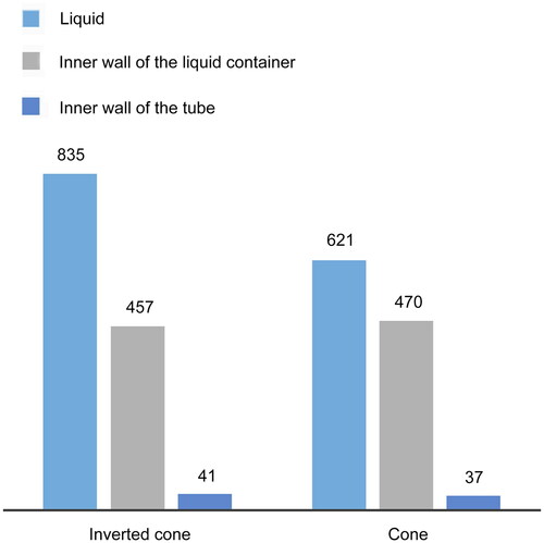
The diameter of the liquid surface meniscus in the inverted conical cup is much larger than that in the conical cup. The contact area between the liquid surface and the air is also large. The probability of collision of particles in the air with the liquid is higher. During the operation of the biological sampler, because the lower space of the inverted conical cup is larger, the liquid can easily rotate and flow. The resulting liquid envelope can seamlessly collect more particles than the conical cup.

Liquid volume

In this study, the bioaerosol sampler collects biological particles using a mechanism that follows the aerosol-to-hydrosol approach. Therefore, we considered the liquid volume as a main design factor. This factor measured from the distance between the air nozzle exit and the top of the liquid surface level. Three different liquid capacities were considered. The distances between the nozzle and the liquid level for the three capacities were 5, 10, and 15 mm, respectively. The liquid volumes were 60, 40, and 20 mL, corresponding to the distances of 5, 10, and 15 mm, respectively. The jet had a different effect on the liquid surface’s point of action for different distances. Thus, the movement state of the air flow was also different. Additionally, the size and density of the air vortex formed above the liquid surface were also different.

The flow-field diagram of the central section for the distances of 5, 10, and 15 mm is shown in Figure 6. A comparison of the flow-field diagrams for the distances of 10 and 15 mm reveals that, when the distance was 15 mm, the diameter of the vortex above the liquid surface was larger than 10 mm, and the air distribution inside the vortex was uniform (Figures 6a and b). At 10 mm, because the liquid level was closer to the nozzle, a large part of the jet from the nozzle impinged on the liquid level, and therefore the force on the liquid at 10 mm was greater than at 15 mm. However, the distance of 15 mm saw the formation of more swirls than for 10 mm. When the distance was 5 mm, the eddy current above the liquid surface was significantly smaller than that for 15 mm and 10 mm (Figure 6c). This may have been caused by the space limitation. However, the liquid surface was too close to the nozzle as the flow rate of air acting on the liquid increased, releasing more bubbles into the liquid. A comparison of the flow-field diagrams with the simulation result of the distance between the nozzle and liquid surface (5 and 10 mm) showed that vortices above the 5-mm liquid surface level were smaller, while those above the 10-mm level were larger with a uniform internal air distribution. At 10 mm, a large amount of air impinged on the liquid, but the bubble diameter was less than 5 mm and the vortex above the liquid surface 10 mm from the nozzle was large and uniform, which facilitated the collection of more particles.

Figure 6. Vector diagram of the central section for distances of 15, 10, and 5 mm between the air nozzle and the liquid surface level: (a) distance of 15 mm between the air nozzle and the liquid surface level; (b) distance of 10 mm between the nozzle and the liquid level; (c) distance of 5 mm between the nozzle and the liquid level.

Based on the above analysis, we conclude that, when the distance between the nozzle and the liquid surface is larger, the space above the liquid surface and the size of the air vortex are larger, and the air distribution inside the vortex is more uniform. In this case, since the liquid level is close to the nozzle, the direct collection of biological particles became possible. As shown in Figure 7, the amount of particles collected by the liquid from a height of 10 mm was greater than those from 5 and 15 mm. Moreover, a similar result was obtained for the inner wall of the liquid container. However, the number of particles in the tube for the distance of 10 mm was less than that for 5 and 15 mm. This indicated that most particles impinged on the liquid container or the wall of the container, traveled along the container wall, and finally were collected by the liquid container from 10 mm. When the nozzle was 10 mm from the liquid level, the particle collection had a larger air flow vortex and a more uniform air distribution, avoiding the release of air bubble. Hence, this distance is ideal for the bioaerosol sampler design.

Figure 7. Histograms of number of particles collected by the liquid when the liquid level is 15, 10, and 5 mm from the air nozzle, as per the CFD simulation. Each histogram includes three bars based on the values from Table 4. (1) Liquid: the total number of particles in the liquid corresponding to each liquid-level distance; (2) inner wall of the liquid container: the total number of particles at the inner wall of the liquid container corresponding to each liquid-level distance; and (3) inner wall of the tube: the total number of particles at the inner wall of the tube corresponding to each liquid-level distance.

Nozzle angles

The three nozzle angles of 30°, 45°, and 60° were considered in the bioaerosol sampler (Figure 8). Figures 8a and c shows that the overall distributions of the air velocity with the nozzle angles of 30° and 45° are similar. The air enters the nozzle, and the speed of the circular pipe with a smaller cross section became larger. As the air passes through the nozzle, its velocity maximizes and forms a jet. Figures 8b and d presents the vectorial and streamline characteristics of the flow field at nozzle angles of 30° and 45°. The figure shows that the air flow enters the sampler through the inlet and forms a large eddy current in the upper section. A portion of the air flow rotates about the circular protruding pipe in the upper section and enters the nozzle through the pipe with the rest of the air flow. In the nozzle, a portion of the air forms an eddy current and is subsequently ejected at a high speed by the nozzle. The motion form and direction of the air flow at the nozzle angle of 30° are essentially the same.

Figure 8. Vector and three-dimensional streamline diagrams of the flow field at nozzle angles of 30°, 45°, and 60°. (a) Vector diagram of the flow field at a nozzle angle of 30°; (b) three-dimensional streamline diagram of the flow field at a nozzle angle of 30°; (c) vector diagram of the flow field at a nozzle angle of 45°; (d) three-dimensional streamline diagram of the flow field at a nozzle angle of 45°; (e) vector diagram of the flow field at a nozzle angle of 60°; and (f) three-dimensional streamline diagram of the flow field at a nozzle angle of 60°.

From Figure 8e, the section velocity of at 60° is larger than those at 30° and 45°, which in this case is related to the vortex velocity. The jet from the 60° nozzle was straighter than those from the 30° and 45° nozzles. The vector diagram (Figure 8e) shows the formation of a small eddy current in the midsection of the 60° nozzle due to the superposition of two eddy currents, which prolongs the residence time of the air flow. Additionally, most of the 60° jet impinging on the liquid surface is vertical, while a portion of the 30° and 45° jet is horizontal (Figure 8f). Owing to extrusion between the air flows, parts of the air flow rotated upward to form a vortex. The vortex formed by the 60° jet was much rarer than that formed by the 30° and 45° ones. The air flow velocity from the distribution in the cup with the 60° nozzle was more than 8 m/s.

From this analysis, an increase in the nozzle angle causes an increase in the amount of air impinging on the liquid in the inverted conical bottle, which increases the turbulence in the liquid. The jet velocity at the nozzle exit is different for different nozzle angles owing to the formation of vortices. Figure 9 shows the number of particles collected by the liquid for the three nozzle angles. Most of the air flowing from the 45° and 60° nozzles made a direct impact on the liquid, which was conducive to the direct collection of particles by the liquid. However, only part of the air flow from the 30° nozzle could make a direct impact on the liquid surface, while another portion rotated upward to impact the inner wall of the cup. This resulted in the accrual of more particles on the inner wall, which then slid into the liquid with the hydrosol drops on the wall. The nozzle angle of 45° (2469) ejected the largest amount of biological particles into the liquid among the three, followed by 60° (2434) and 30° (1969). Therefore, angle 45°, 10 mm, inverted cone vessel shape, 45° nozzle is the best configuration.

Figure 9. Histogram of the number of particles collected by the container for the three nozzle angles in liquid, and the inner walls of the liquid container and the tube from the CFD simulation. Each group includes three bars based on the values from Table 4. (1) Liquid: the total number of particles in the liquid at each distance of the liquid surface from the nozzle; (2) Inner wall of the liquid container: the total number of particles on the inner wall of the liquid container at each distance; and (3) Inner wall of the tube: the total number of particles on the inner wall of the tube at each distance.

Field experiment

The first (angle 45°, 10 mm, inverted cone) and second-best optimized samplers (angle 60°, 10 mm, inverted cone) were 3 D-printed and used in a field experiment (Figure 10). The design is illustrated in Figure 11. The results showed that the duplicate results with angle 45°, 10 mm and inverted cone configuration (Figures 12e and f) had 17 CFU/plate and 8 CFU/plate. The angle 60°, 10 mm and inverted cone configuration (Figures 12b and c) had 13 CFU/plate and 2 CFU/plate. The positive control group contained naturally collected biological particles without the use of the sampler (Figure 12a), while the negative control group contained 1XPBS to capture the particles (Figure 12d). The on-field data evaluated the best optimized sampler (angle 45°, 10 mm and inverted-cone collection cup) with the best collection capacity, followed by the second-best one (angle 60°).

Figure 10. Three-dimensional printed prototype of inverted-cone and cone vessels.

Figure 11. Three-dimensional printed prototypes for two selected optimized cases under different conditions: (a) angle of 45°, distance of 10 mm, cone in static condition; (b) angle of 45°, distance of 10 mm, cone in operating condition; (c) angle of 45°, distance of 10 mm, inverted cone in static condition; (d) angle of 45°, distance of 10 mm, inverted cone in working condition; (e) angle of 60°, distance of 10 mm, cone in static condition; (f) angle of 60°, distance of 10 mm, cone in working condition; (g) angle of 60°, distance of 10 mm, inverted cone in static condition; and (h) angle of 60°, distance of 10 mm, inverted cone in working condition.

Figure 12. Field experiment with the two best geometrically optimized samplers (angle 45°, 10 mm, inverted cone; and angle 60°, 10 mm, inverted cone). (a) natural collection of biological particles without biological sampler (positive control); (b) angle 60°, 10 mm, inverted cone; (c) duplicate: angle 60°, 10 mm, inverted cone; (d) PBS as the negative control group; (e) angle 45°, 10 mm, inverted cone; and (f) duplicate: angle 45°, 10 mm, inverted cone.

Uncertainties and limitations

This study used the orthogonal design method to optimize the geometrical parameters and reduce the computational time of the CFD simulation. However, like existing studies, the CFD models in this article are still based on finite element methods, and hence consider numerous parameters. These models required long computational time and had data divergence (Kim, Hur, and Kim 2012). It is typically quite difficult to setup the boundary between different media in CFD simulations, particularly in a three-phase flow. Additionally, CFD is a macroscale simulation technique and cannot perform accurate microscale calculations, such as those related to small-size particles in nano- or micro-meter scale including airborne bacteria, viruses, or fungi. Therefore, future studies should consider developing a fast and accurate three-phase numerical simulation with a clear boundary and fast convergence to simulate parameters of air, particles, and liquid media, and guide the optimization of the bioaerosol sampler design with the goal of highest possible sampling efficiency.

In addition, the field experiment focused on the collection of bacteria only ran two iterations for each of the two biological samplers at one sampling site. More accumulative sampling and diversified bioaerosol targets (fungi or viruses) in both the laboratory and field environments are necessary to obtain larger volumes of data for verifying the optimized biological sampler design in the future.

The particle-size selection has an impact on the geometric design of the sampler. However, this is only a suggestive result for the optimization of the physical geometry of the sampler. Although the CFD simulation of the samplers revealed that the sampler had the highest collection efficiency when accumulating 10-µm-diameter particles, it was only a preliminary result of the virtual situation. We could not confirm that the particle size was indeed a direct factor affecting the geometric design in practice. In the future study, the particle size-related optimized geometric parts could be an input parameter of the design, not just using the different particle size as indicators to verify the collection efficiency of a designed biological sampler. Future experiments must refine the selection criterion of parameters and values given in this study. Moreover, this study does not include a few other parameters that are also important for the design of a sampler (e.g., pressure drop, particle weight, air flow rate, liquid flow rate, flow type [laminar/turbulent]). This study considers the feasibility of conducting follow-up field experiments and does not involve continuous parameters. By considering more continuous values for each parameter in the next step, and the correlation between each parameter, we may obtain more results.

Conclusions

This study developed an orthogonal design method to optimize the geometric parameters of a bioaerosol sampler. It used a three-dimensional CFD approach to predict the particle-capture characteristics and the four crucial parameters (particle size, nozzle angle, liquid container shape, and distance between the nozzle and the liquid surface) of an aerosol-to-hydrosol biological sampler. Three-dimensional printing was used to make the prototypes based on the optimized geometrical design and implemented them in a field experiment, to validate the bioaerosol samplers’ capturing efficiency. The conclusions drawn from this study are as follows:

1. The best combination of parameters for a bioaerosol sampler according to the orthogonal experimental analysis is: particle size: 10 µm, geometry: inverted cone, distance: 10 mm, and angle: 45°.

2. The particle path and capturing rate simulations will guide the future geometrical optimization of biological samplers.

3. The on-field sampling experiment verified that the case with a nozzle angle of 45° and a liquid level-to-nozzle distance of 10 mm, and an inverted-cone shape had the best particle-collection capacity, followed by the second-best case with an angle of 60°, a distance of 10 mm, and an inverted-cone-shaped collection cup.

Nomenclature
η	=	particle deposition percentage
S1	=	total number of particles entering the biological sampler
S2	=	number of particles entering the liquid
k	=	turbulent kinetic energy
ε	=	turbulent kinetic energy dissipation rate
Gk	=	generation term of turbulent kinetic energy k caused by the average velocity gradient
Gb	=	generation term of turbulent kinetic energy k caused by the buoyancy
YM	=	proportion of dissipation caused by fluid pulsation expansion in compressible turbulence to total dissipation
C1ε	=	empirical constants
C2ε	=	empirical constants
C3ε	=	empirical constants
αK	=	reciprocal of effective Prandtl number corresponding to turbulent energy k
αε	=	reciprocal of effective Prandtl number corresponding to dissipation rate ε
Sk	=	user-defined terms
Sε	=	user-defined terms
Sαq	=	source term of mass
Keff	=	effective thermal conductivity
Sh	=	source term, including radiation and other volume heat sources
E	=	total energy
Ui	=	instantaneous velocity of air
Upi	=	instantaneous velocity of particles
µ	=	molecular viscosity of air
ρ	=	air and particle densities
dp	=	particle size
Re	=	particle Reynolds number
CD	=	drag coefficient
gi	=	acceleration due to gravity in the i direction
Fai	=	additional force on particles in the i direction
du/dy	=	velocity gradient of the air flow in space
Vpx	=	force of particles moving in the axial direction
Ki	=	sum of capture rate for factor “angle,” where “i” is the level from each factor

Acknowledgment

We gratefully acknowledge the support provided by the personnel involved in the experiments.

Disclosure statement

The authors declare that they have no conflicts of interest.

Additional information

Funding

This work was supported by the Chinese Academy of Inspection and Quarantine under Grant 2018JK015.

References

- Arruda, A. G., S. Tousignant, J. Sanhueza, C. Vilalta, Z. Poljak, M. Torremorell, C. Alonso, and C. Corzo. 2019. Aerosol detection and transmission of porcine reproductive and respiratory syndrome virus (PRRSV): What is the evidence, and what are the knowledge gaps? Viruses 11 (8):712. doi:https://doi.org/10.3390/v11080712.
- Balestrin, E., R. K. Decker, D. Noriler, J. C. S. C. Bastos, and H. F. Meier. 2017. An alternative for the collection of small particles in cyclones: Experimental analysis and CFD modeling. Separation & Purification Technology 184:54–65. doi:https://doi.org/10.1016/j.seppur.2017.04.023.
- Baron, P. A., Kulkarni, P., and Willeke, K. 2011. Aerosol measurement: principles, techniques, and applications. Eds. 3rd ed. Hoboken, N.J: Wiley.
- Black, R. S., and M. J. Shaw. 2002. Development of the wetted wall cyclone collector. Proceedings of the Scientific Conference on Obscuration and Aerosol Research.
- Boysan, F., Ayers, W. H., and Swithenbank, J. A. 1982. A Fundamental Mathematical Modelling Approach for Cyclone Design. Trans. Inst. Chem. Engin 60:222–230.
- Cho, Y. S., S. C. Hong, J. Choi, and J. H. Jung. 2019. Development of an automated wet-cyclone system for rapid, continuous and enriched bioaerosol sampling and its application to real-time detection. Sensors and Actuators B: Chemical 284:525–33. doi:https://doi.org/10.1016/j.snb.2018.12.155.
- Dean, A., and D. Voss. 1999. Design and analysis of experiments. Berlin, Germany: Springer.
- Deng, L.-Y. 2000. Orthogonal arrays: Theory and applications. Technometrics 42 (4):440. doi:https://doi.org/10.1080/00401706.2000.10485735.
- Després, V., J. A. Huffman, S. M. Burrows, C. Hoose, A. Safatov, G. Buryak, J. Fröhlich-Nowoisky, W. Elbert, M. Andreae, U. Pöschl, et al. 2012. Primary biological aerosol particles in the atmosphere: A review. Tellus B: Chemical and Physical Meteorology 64 (1):15598. doi:https://doi.org/10.3402/tellusb.v64i0.15598.
- Dirgo, J., and D. Leith. 1985. Cyclone collection efficiency: Comparison of experimental results with theoretical predictions. Aerosol Science and Technology 4 (4):401–415. doi:https://doi.org/10.1080/02786828508959066.
- Griffiths, W. D., and Boysan, F. 1996. Computational Fluid Dynamics (CFD) and Empirical Modeling of a Number of Cyclone Samplers. Journal of Aerosol Science 7(2):281–304.
- Haig, C. W., W. G. Mackay, J. T. Walker, and C. Williams. 2016. Bioaerosol sampling: Sampling mechanisms, bioefficiency and field studies. Journal of Hospital Infection 93 (3):242–55. doi:https://doi.org/10.1016/j.jhin.2016.03.017.
- Hedayat, A. S., N. J. Sloane, and J. Stufken. 1999. Orthogonal arrays: Theory and applications. Berlin, Germany: Springer-Verlag.
- Judson, S. D., and V. J. Munster. 2019. Nosocomial transmission of emerging viruses via aerosol-generating medical procedures. Viruses 11 (10):940. doi:https://doi.org/10.3390/v11100940.
- Kenny, L. C., A. Thorpe, and P. Stacey. 2017. A collection of experimental data for aerosol monitoring cyclones. Aerosol Science and Technology 51 (10):1190–200. doi:https://doi.org/10.1080/02786826.2017.1341620.
- Kessler, M., and D. Leith. 1991. Flow measurement and efficiency modeling of cyclones for particle collection. Aerosol Science and Technology 15 (1):8–18. doi:https://doi.org/10.1080/02786829108959508.
- Kim, J.-H., N. Hur, and W. Kim. 2012. Development of algorithm based on the coupling method with CFD and motor test results to predict performance and efficiency of a fuel cell air fan. Renewable Energy 42:157–62. doi:https://doi.org/10.1016/j.renene.2011.08.029.
- King, M. D., and A. R. McFarland. 2012. Bioaerosol sampling with a wetted wall cyclone: Cell culturability and DNA integrity of Escherichia coli bacteria. Aerosol Science and Technology 46 (1):82–93. doi:https://doi.org/10.1080/02786826.2011.605400.
- Kulkarni, P., P. A. Baron, C. M. Sorensen, and M. Harper. 2011. Nonspherical particle measurement: Shape factor, fractals, and fibers. In Aerosol measurement: Principles, techniques, and applications, eds. P. Kulkarni, P. A. Baron, and K. Willeke, 507–47. Hoboken, NJ: John Wiley & Sons. doi:https://doi.org/10.1002/9781118001684.ch23.
- Langer, V., G. Hartmann, R. Niessner, and M. Seidel. 2012. Rapid quantification of bioaerosols containing L. pneumophila by Coriolis® µ air sampler and chemiluminescence antibody microarrays. Journal of Aerosol Science 48:46–55. doi:https://doi.org/10.1016/j.jaerosci.2012.02.001.
- Lee, I.-B., Bitog, J. P. P., Hong, S.-W., Seo, I.-H., Kwon, K.-S., Bartzanas T., and Kacira, M. 2013. The past, present and future of CFD for agro-environmental applications. Computers & Electronics in Agriculture 93: 168–183.
- Li, G., S. Yu, X.-S. Yang, and Q.-F. Chen. 2011. Study on extraction technology for chlorogenic acid from sweet potato leaves by orthogonal design. Procedia Environmental Sciences 8:403–7. doi:https://doi.org/10.1016/j.proenv.2011.10.063.
- Montgomery, D. C. 2020. Design and analysis of experiments. 10th ed. Hoboken, NJ: John Wiley & Sons.
- Noh, S.-Y., J.-E. Heo, S.-H. Woo, S.-J. Kim, M.-H. Ock, Y.-J. Kim, and S.-J. Yook. 2018. Performance improvement of a cyclone separator using multiple subsidiary cyclones. Powder Technology 338:145–152. doi:https://doi.org/10.1016/j.powtec.2018.07.015.
- Peng, W., A. C. Hoffmann, H. Dries, M. Regelink, and K.-K. Foo. 2007. Reverse-flow centrifugal separators in parallel: Performance and flow pattern. AIChE Journal 53 (3):589–97. doi:https://doi.org/10.1002/aic.11121.
- Song, J., Y. Zhang, D. Zhu, and R. Xiang. 2019. Performance evaluation of virtual cyclone with various inlet and outlet dimensions. Journal of Aerosol Science 128:114–24. doi:https://doi.org/10.1016/j.jaerosci.2018.12.002.
- Syed, M. S., M. Rafeie, R. Henderson, D. Vandamme, M. Asadnia, and M. E. Warkiani. 2017. A 3D-printed mini-hydrocyclone for high throughput particle separation: Application to primary harvesting of microalgae. Lab on a Chip 17 (14):2459–69. doi:https://doi.org/10.1039/c7lc00294g.
- Tellier, R., Y. Li, B. J. Cowling, and J. W. Tang. 2019. Recognition of aerosol transmission of infectious agents: a commentary. BMC Infectious Diseases 19 (1):101. doi:https://doi.org/10.1186/s12879-019-3707-y.
- Van Doremalen, N., T. Bushmaker, D. H. Morris, M. G. Holbrook, G. Amandine, B. N. Williamson, A. Tamin, J. H. Harcourt, N. J. Thornburg, S. I. Gerber, et al. 2020. Aerosol and surface stability of SARS-CoV-2 as compared with SARS-CoV-1. The New England Journal of Medicine 382 (16):1564–1567. doi:https://doi.org/10.1056/NEJMc2004973.
- Villi, G., and M. De Carli. 2014. Detailing the effects of geometry approximation and grid simplification on the capability of a CFD model to address the benchmark test case for flow around a computer simulated person. Building Simulation 7 (1):35–55. doi:https://doi.org/10.1007/s12273-013-0103-1.
- Vincent, J. H. 2007. Aerosol sampling: Science, standards, instrumentation and applications. Chichester, UK: John Wiley & Sons.
- Vinchurkar, S., P. W. Longest, and J. Peart. 2009. CFD simulations of the Andersen cascade impactor: Model development and effects of aerosol charge. Journal of Aerosol Science 40 (9):807–22. doi:https://doi.org/10.1016/j.jaerosci.2009.05.005.
- Wang, X., Yang, Z., and Duan, L. 2007. About some optimization design problems of ANSYS. Journal of Plasticity Engineering 14(6): 181–184.
- Willeke, K., X. Lin, and S. A. Grinshpun. 1998. Improved aerosol collection by combined impaction and centrifugal motion. Aerosol Science and Technology 28 (5):439–56. doi:https://doi.org/10.1080/02786829808965536.
- Wubulihairen, M., X. Lu, P. K. H. Lee, and Z. Ning. 2015. Development and laboratory evaluation of a compact swirling aerosol sampler (SAS) for collection of atmospheric bioaerosols. Atmospheric Pollution Research 6 (4):556–61. doi:https://doi.org/10.5094/apr.2015.062.
- Yoo, K., T. K. Lee, E. J. Choi, J. Yang, S. K. Shukla, S.-I. Hwang, and J. Park. 2017. Molecular approaches for the detection and monitoring of microbial communities in bioaerosols: A review. Journal of Environmental Sciences (China) 51:234–47. doi:https://doi.org/10.1016/j.jes.2016.07.002.
- Zeng, B., H. D. Yan, L. K. Huang, Y. C. Wang, J. H. Wu, X. Huang, A. L. Zhang, C. R. Wang, and Q. Mu. 2016. Orthogonal design in the optimization of a start codon targeted (SCoT) PCR system in Roegneria kamoji Ohwi. Genetics and Molecular Research 15 (4):gmr15048968. doi:https://doi.org/10.4238/gmr15048968.
- Zhou, L. X., and Soo, S. L. 1990. Gas-solids Flow and Collection of Solids in a Cyclone Separator. Powder Technol 63:45–53.