Impact of combustion conditions on physical and morphological properties of biomass burning aerosol

Abstract

The study of biomass burning particle density provides information on aging, new particle formation, transport properties, and is an important parameter in aerosol impacts modeling. Density is used in mass closure techniques to estimate the temporal resolution of particulate mass concentrations. However, the study of BB particle density as a function of burning conditions is still limited. Laboratory measurement of six sub-Saharan African biomass fuels burned under a range of conditions, from pure smoldering to pure flaming conditions, is presented. Smoldering-dominated burning (modified combustion efficiency (MCE) < 0.9) particles has a very narrow range of effective density (${\rho }_{\mathit{eff}}$) 1.03 g cm⁻³ to 1.21 g cm⁻³ and a mass mobility exponent ($D_{fm}$) of ∼3 (2.97 ± 0.05), indicating that they are spherical particles. For the flaming-dominated burning (MCE >0.95) particles, show a size dependent ${\rho }_{\mathit{eff}}$ for all six different fuels. In this case, the mean and standard deviation of the ${\rho }_{\mathit{eff}}$ decreased with increasing size, from (0.94 ± 0.21) g cm⁻³ at a mobility diameter of 80 nm to (0.31 ± 0.07) g cm⁻³ at a mobility diameter of 400 nm. The size-dependent ${\rho }_{\mathit{eff}}$ of flaming-dominated aerosol suggests the fractal nature of freshly emitted particles. The relationship between $D_{fm}$ and the MCE shows three distinct morphology regimes, which we define as the spherical particle, the transition, and the fractal regime. Our proposed relationship of $D_{fm}$ with the MCE can be used as a tool to assess the applicability of Mie theory for optical closure calculations in the absence of particle morphological information.

EDITOR:

• Hans Moosmüller

1. Introduction

Emissions from biomass burning (BB) are one of the major sources of atmospheric aerosol loading (Bond et al. 2004, 2013). BB emissions impact regional and global weather, climate, air quality, and human health. Open BB is a major source of atmospheric black carbon (BC) and organic carbon (OC), accounting for 42% and 74% of atmospheric BC and OC loading, respectively (Bond et al. 2004). Even though warming due to BC from BB is offset by cooling due to OC and other inorganic aerosol, with a net radiative forcing of 0 Wm⁻², the uncertainty in the estimate lies between −0.2 Wm⁻² and +0.2 Wm⁻² (IPCC 2013). BC is the main light-absorbing aerosol with an estimated positive radiative forcing only second to carbon dioxide (Bond et al. 2013; Jacobson 2001). However, there is a large uncertainty with regards to the forcing due to BC, with an average forcing of +0.71 Wm⁻² with a 90% bound ranging from +0.08 Wm⁻² to 1.27 Wm⁻² (Bond et al. 2013). The forcing due to BC is largely influenced by the mixing state and morphology of the particles. The emissions from BB are mostly dominated by organic aerosol (OA). The fraction of OA commonly known as brown carbon (BrC) shows enhanced absorption at lower visible and ultraviolet wavelengths (Pokhrel et al. 2017; Laskin, Laskin, and Nizkorodov 2015; McMeeking et al. 2014; Saleh et al. 2014; Kirchstetter and Thatcher 2012; Lack et al. 2012). The positive forcing due to BrC is found to be non-negligible compared to BC at the top of the atmosphere (Brown et al. 2018; Wang et al. 2018). This fact suggests that a more accurate estimation of forcing due to BrC is necessary to reduce the uncertainty in the net radiative forcing. However, most experimentally determined absorption measurements are performed on bulk aerosol, which includes both BC and BrC. Absorption due to BrC is estimated by subtracting the absorption due to BC from the bulk absorption of both BC and BrC. So, to more accurately estimate the absorption due to BrC, an accurate measurement of BC absorption is needed. Calculation of BC absorption using optical models requires input parameters such as size distribution, mixing state, and morphology of the BC. Mie theory (Bohren and Huffman 1983) is the most commonly used approach to estimate the BC absorption (Saliba et al. 2016; Saleh et al. 2013, 2014; Cappa et al. 2012), which does not take into account the fractal nature of BC and can result in a bias in the estimated BC absorption and uncertainty in the estimated optical properties of BrC.

One of the most common ways to estimate atmospheric particle material density is by measuring the aerosol’s chemical composition (Vakkari et al. 2014). However, a complete measurement of the chemical composition of atmospheric aerosol requires extensive instrumentation. With the invention of the differential mobility analyzer (DMA) (Liu and Pui 1974), the electrical mobility diameter ($d_m)$ is the most common way to measure particle size. However, for non-spherical particles, $d_m$ is not equal to the geometric diameter and estimating the true material density requires an accurate measurement of particle mass, $d_m,$ and the dynamic shape factor. Therefore, an alternative particle property called its effective density (${\rho }_{\mathit{eff}}$), defined as the ratio of particle mass to the volume of its mobility equivalent sphere, has been commonly used in aerosol studies (Sumlin et al. 2018; Qiao et al. 2018; Li et al. 2016; Rissler et al. 2014; Park, Kittelson, and McMurry 2004; Maricq and Xu 2004; Park et al. 2003a; McMurry et al. 2002). The effective density of atmospheric particles is an important property, since it is linked not only to the particle’s emission sources and aging process, but also to its physical, microphysical, and optical properties (Zhao et al. 2019). The effective density is also impacted by the particle morphology, mixing state, and the chemical composition.

Particles emitted from BB emissions have a complex morphology. The common technique used to characterize particle morphology is transmission electron microscopy and scanning electron microscopy (Sarpong et al. 2020; Girotto et al. 2018; Chakrabarty et al. 2014; China et al. 2013; Park, Kittelson, and McMurry 2004, Park et al. 2003a). However, none of these techniques can provide continuous online information regarding particle morphology. The relationship between size-selected effective density and $d_m$ can predict the complex morphology of the particles in real-time (Park, Kittelson, and McMurry 2004, Park et al. 2003a). Furthermore, the time evolution of ${\rho }_{\mathit{eff}}$ can provide information regarding the atmospheric processing of aerosol, since ${\rho }_{\mathit{eff}}$ changes due to chemical reactions, new particle formation, and restructuring of fractal agglomerates (Pagels et al. 2009; Katrib et al. 2005). The size-resolved ${\rho }_{\mathit{eff}}$ can also be used to determine the high temporal resolution of the mass concentration from the ambient particle number size distribution measured by a scanning mobility particle sizer (SMPS) for the study of air quality and visibility (McMurry et al. 2002).

Even though the DMA-particle mass analyzer system is very popular in determining the ${\rho }_{\mathit{eff}}$ of engine exhaust particles (Olfert et al. 2017; Park, Kittelson, and McMurry 2004; Maricq and Xu 2004; Sakurai et al. 2003; Park et al. 2003a) and ambient aerosols (Wu et al. 2019; Qiao et al. 2018; Rissler et al. 2014), the ${\rho }_{\mathit{eff}}$ measurement of primary aerosol emitted from BB are still limited (Sumlin et al. 2018; Zhai et al. 2017; Li et al. 2015). Most of the studies that determined aerosol mass from the particle size distribution applied an assumed density ranging from 1.0 g cm⁻³ to 1.7 g cm⁻³ regardless of the diameter, aging conditions, and morphology of the particles (Corbin et al. 2019; Kumar et al. 2018; Gkatzelis et al. 2016; Saliba et al. 2016; Vakkari et al. 2014; Flowers et al. 2010). An accurate measurement of particle density is also necessary from the climate model perspective, since climate models estimate the refractive indices of total aerosol as a volume-weighted refractive index (Brown et al. 2018; Liu et al. 2012). In addition, it is found that the density of OA plays a significant role in the estimated aerosol radiative forcing and aerosol-cloud interactions in climate models (Brown et al. 2018).

In this study, we performed laboratory combustion experiments on six different sub-Saharan African biomass fuels, to study the physical and morphological properties under a variety of burning conditions ranging from purely smoldering to purely flaming. In this article, we investigate how burning conditions impact the physical properties of the emitted aerosol, namely the ${\rho }_{\mathit{eff}},$ the particle size distribution, and a morphological property (mass mobility exponent). We also show the relationship between mass mobility exponent and the modified combustion efficiency, which could be used as a tool to access the applicability of Mie-based modeling for aerosol emitted under different burning conditions.

2. Materials and method

2.1. NCAT burning facility

This work was conducted at the North Carolina Agricultural and Technical State University (NCAT) indoor burning facility that has a well-equipped environmental chamber for the measurement of fresh and aged aerosol, which is described in detail elsewhere (Smith et al. 2019, 2020a, 2020b). BB aerosol was generated by the combustion of biomass fuel in a tube furnace. The furnace (Carbolite Gero, HST120300-120SN) holds an 85 mm OD, 80 mm ID, and 750 mm long quartz working tube with a heated region of 300 mm. House compressed air that passes through a zero-air generator (Aadco Instruments, 747-30) is used to provide zero air to the tube furnace through stainless steel tubing. The flowrate (10 standard liters per minute) of zero air was controlled by mass flow controller (MFC, Sierra Instruments) calibrated using flow calibrator (MesaLabs, Definer 220). The desirable mass of the biomass fuel sample was placed in a quartz combustion boat (AdValue Technology, FQ-BT-03) and placed at the center of the furnace for the ignition. The temperature of the furnace can be adjusted from room to 1000 °C as desired. The smoke produced during combustion was sent to the indoor smog chamber via a heated (200 °C), ¼ inch stainless steel transfer tube. The NCAT environmental chamber has a volume of 9.01 m³ and is lined by ethylene propylene (FEP) Teflon. There are 64 ultraviolet lights (Sylvania, F30T8/350BL/ECO, 36") on two sides (32 on each) for the photochemical aging experiments. A mixing fan is located inside of the reactor, which generally produces a well-mixed volume within 15 to 20 min after combustion. Typically, the furnace was disconnected 10 min after the start of ignition and the chamber was constantly diluted by zero air. During this study, a dilution flow of 4 L min⁻¹ was used but could be varied depending on instrument sampling flow. The relative humidity inside the chamber was monitored (Traceable Products, Model 4085; humidity range 5% to 95%) and was found to be always below the detection limit of our instrument. The temperature inside the chamber was typical laboratory temperature, which ranged from 21 °C–24 °C. The schematic of the NCAT chamber facility and measurement setup is shown in Figure 1.

Figure 1. Schematic of NCAT chamber facility and measurement setup for physical and morphological properties measurements.

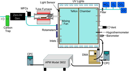
After a series of measurements were complete, the smog chamber was flushed with zero air at a flow rate of 15 L min⁻¹–20 L min⁻¹ for at least 24 h. In addition, lights were turned on to effectively remove NOx. The furnace was also cleaned to remove any remaining residue in the furnace by heating it to 800 °C for at least 2 h. In addition, the tube connecting the furnace to the chamber was also cleaned with methanol after each experiment. Before each burn, chamber pressure and background aerosol/gas concentration were flushed and monitored to make sure that it was clean before proceeding with another experiment. Typically, particle masses below 2 µg m⁻³ and NO and O₃ concentrations of less than 5 ppbv were considered as best conditions to start a new experiment.

2.2. Sample preparation

Woody biomass fuels were obtained from Ethiopia and Botswana and stored under the fume hood to dry. A calibrated analytical balance was used to measure the mass of the fuel that was burned. Typically, we burned less than one gram of fuel except under some occasions when a higher mass load was needed. Fuel moisture content was estimated by measuring mass loss in the fuel due to overnight heating in the oven set at 90 °C. Fuel moisture (FM) is estimated as dry mass fraction as: (1) $$\mathrm{FM}=\mathrm{ }\left(\frac{m_{\mathit{wet}}-m_{\mathit{dry}}}{m_{\mathit{dry}}}\right)\times 100\mathrm{\%}$$(1) where $m_{\mathit{wet}}$ is fuel mass before heating and $m_{\mathit{dry}}$ is fuel mass after heating overnight (Christian et al. 2003). The estimated fuel moisture content for all the fuels used in this study was less than 10%. A list of fuels burned, the geographic location of each fuel, and their burning conditions are presented in Table S1.

2.3. Modified combustion efficiency

Fuel geometry (that includes volume to surface ratio and orientation), moisture content, and environmental variables impact the emissions from fire. The modified combustion efficiency (MCE) is calculated to quantify the relative stage of flaming and smoldering of a fire during burning. (2) $$\mathrm{MCE}=\frac{{\Delta CO}_2}{\Delta CO+{\Delta CO}_2}$$(2) where ${\Delta CO}_2$ and $\Delta CO$ are the background-corrected carbon dioxide and carbon monoxide concentrations, respectively (Stockwell et al. 2014; Yokelson et al. 1997). Typically, MCE values of ∼0.99 are attributed to purely flaming burns and those with values of ∼0.8 or less to purely smoldering burns. An MCE of ∼0.9 represents equal contributions of the flaming and smoldering stages (Stockwell et al. 2014). To achieve the different combustion conditions, furnace temperature was adjusted between 450 °C to 800 °C. It was found that the MCE of lower temperature burns (450 °C to 500 °C) were below 0.90 whereas MCE of high temperature burns (700 °C and 800 °C) were greater than 0.95. CO and CO₂ concentrations were measured by a CO analyzer (model 48 C Thermo Scientific) and a CO₂ analyzer (model 41 C Thermo Scientific). These monitors were calibrated using certified standard gas cylinders (199.7 ppmv for CO and 5028 ppmv for CO₂ from Airgas National Welders).

2.4. Particle morphology and effective density

For non-spherical particles, the estimation of material density is only possible once the dynamic shape factor, porosity and chemical composition are known. Due to limitations in accurately measuring the dynamic shape factor, the particle effective density was introduced as a ratio of the particle mass ($m_p$) to the mobility diameter equivalent volume (volume calculated assuming a spherical particle with a diameter equal to the mobility diameter ($d_m$)) (DeCarlo et al. 2004; Park et al. 2003a; McMurry et al. 2002). ${\rho }_{\mathit{eff}}$ can be expressed as: (3) $${\rho }_{\mathit{eff}}=\frac{6m_p}{\pi {d_m}^3}$$(3) for spherical particles without internal voids and the effective density is equal to its material density for single component systems. However, for non-spherical particles and spherical particles with internal voids, the effective density is always smaller than material density (McMurry et al. 2002). The mass mobility exponent relation can be expressed as a power-law relationship between $m_p$ and $d_m$ (4) $$m_p=C{d}_m^{D_{fm}}$$(4) where C is a pre-factor and $D_{fm}$ is the mass mobility exponent (Sumlin et al. 2018; Radney and Zangmeister 2016; Park, Kittelson, and McMurry 2004, Park et al. 2003a). $D_{fm}$ is commonly used to describe the particle morphology, with a value ∼3 for spherical particles and <3 for non-spherical particles (Wu et al. 2019; Park, Kittelson, and McMurry 2004, Park et al. 2003a; McMurry et al. 2002). Furthermore, $D_{fm}$ can be converted to the fractal dimension, which is estimated from transmission electron microscopy image analysis (Park, Kittelson, and McMurry 2004).

By combining Equations (3)(3) $${\rho }_{\mathit{eff}}=\frac{6m_p}{\pi {d_m}^3}$$(3) and (4)(4) $$m_p=C{d}_m^{D_{fm}}$$(4) , ${\rho }_{\mathit{eff}}$ can be expressed as follows: (5) $${\rho }_{\mathit{eff}}=\frac{6C{d}_m^{D_{fm}}}{\pi {d_m}^3}=C\mathrm{\prime }{d}_m^{D_{fm}-3}$$(5) where $C^{\mathrm{\prime }}=\frac{6C}{\pi }$ is a constant. For homogeneous spherical particles, $D_{fm}$ ∼3 and the effective density is independent of the particle’s sizes; whereas, for non-spherical, $D_{fm}$ < 3 resulting in the decrease of the effective density as particle size increases.

2.5. DMA-APM system and effective density calculation

SMPS consisting of DMA (Model 3081; TSI Inc.) and a general-purpose water-based condensation particle counter (WCPC; Model 3787; TSI Inc.) was used to measure the particle size distribution of BB aerosol. In another configuration, the aerosol size was selected by the DMA, based on its electrical mobility, and then passed through the aerosol particle mass analyzer (APM; Model 3602; Kanomax Inc.) which classified the aerosols based on the particle mass to charge ratio. This mass to charge selection is accomplished when particles pass through the rotating cylinders of the APM when the radial electrical and centrifugal forces balance each other. The APM was followed by a WCPC. Details of the operating principle of the APM can be found elsewhere (Park, Kittelson, and McMurry 2003b, Park et al. 2003a; McMurry et al. 2002). During this study, APM was operated in stepping mode where rotational speed of the APM was kept constant and voltage was changed stepwise for a selected size to determine the distribution of the particle mass. The classification performance parameter, which is defined as the ratio of the timescale for axial and radial particle movements in the classification zone, was kept fixed (λ = 0.32) during this study. The effective density was estimated for each particle size using Equation (3)(3) $${\rho }_{\mathit{eff}}=\frac{6m_p}{\pi {d_m}^3}$$(3) and the reported effective density values are the peaks of the distribution as shown in Figure S1 (see the online supplementary information [SI]). Based on the recent study by Radney and Zangmeister (2016) on flame-generated soot, the presence of q > +1 would bias the peak of the mass distribution by 13% compared to q = +1 at 150 nm size. This would result in an effective density overestimated by 13%. They concluded that 150 nm diameter particles are the worst-case scenario for charge state separation. For particles smaller than 150 nm the contribution from q > +1 would be minimal, and for particles larger than 150 nm the effective mass separation between successive charge states is large, leading to less bias in the resulting density measurements.

The effective density, calculated using Equation (3)(3) $${\rho }_{\mathit{eff}}=\frac{6m_p}{\pi {d_m}^3}$$(3) , can be impacted by the uncertainty in the mobility diameter selected by DMA. A small error in $d_m$ leads to a large error in the estimated density due to d_m³ term in denominator (Park, Kittelson, and McMurry 2003b; McMurry et al. 2002). To minimize this error, DMA size measurements were first calibrated using polystyrene latex spheres (PSL) for multiple sizes, and a correction factor was applied based on these measurements. The effective density measurement capability of DMA-APM was tested with different PSL particle sizes (${\rho }_{\mathit{eff}}=1.05$ g cm⁻³). The average ${\rho }_{\mathit{eff}}$ estimated by the DMA-APM system for four different PSL sizes was (1.060 ± 0.016) g cm⁻³, where the error is one standard deviation of the average value. The effective density of the different sizes PSL particles measured by the DMA-APM system is shown in Figure S2.

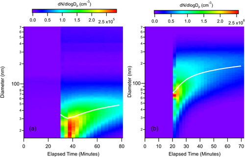
Figure 2. The evolution of the particle size distribution for (a) flaming-dominated and (b) smoldering-dominated eucalyptus burning. The white line indicates the evolution of the geometric mean diameter of the distribution.

3. Result and discussion

3.1. Particle size distribution

The size distribution of the particles emitted during each burn was measured by an SMPS. Typically, the particle size distribution was measured for the first 45–50 min for each experiment before switching to density measurements. Figure 2 shows the time evolution of number size distribution inside the chamber. As expected, there occurred a decrease in particle number concentration and an increase in geometric mean diameter due to diffusional losses to the chamber walls and particle coagulation in the chamber. There existed a clear difference in the particle size distribution of the emitted aerosol under different burning conditions for the same fuel. For the flaming-dominated burn of eucalyptus (MCE = 0.96), size distribution was dominated by ultrafine particles with a geometric mean diameter (GMD) of ∼40 nm, as shown in Figure 2a. Whereas, for the smoldering- dominated burn of eucalyptus (MCE = 0.89), the size distribution was dominated by larger size particles a with GMD >100 nm once the chamber was well mixed (typically 15-20 min after ignition).

This result was consistent with a previous laboratory study (Carrico et al. 2016), which found smoldering fires produced particles that were strongly light scattering, with the size distribution dominated by particles larger than 100 nm, whereas flaming fires produced highly absorbing particles that were dominated by 50 nm particles. In addition, they observed size distributions from the flaming-dominated fires that were bimodal, with a second peak at larger sized particles, while such a feature was absent in smoldering-dominated burning cases.

3.2. Size selected effective density of flaming and smoldering emissions

The effective density of size-selected aerosol was calculated for aerosol generated under different combustion conditions. The temperature of the furnace was adjusted to different temperatures ranging from 450 °C to a maximum of 800 °C. The burning condition was quantified by calculating MCE of the burn and it was found that lower temperature burns (450 °C to 500 °C) were mostly dominated by smoldering emissions (MCE < 0.9) while high temperature burns (700 °C and 800 °C) were dominated by flaming emissions (MCE > 0.95). Figure 3 shows the ${\rho }_{\mathit{eff}}$ plotted as a function of mobility diameter for six different fuels. From the six different fuels with twelve independent burns, it is apparent from Figure 3 that variability in ${\rho }_{\mathit{eff}}$ of smoldering-dominated emissions is within ∼20% of each other. The list of fuels, ${\rho }_{\mathit{eff}},$ and MCE values are presented in Table S2 (SI). Even though there is some fuel type dependency, with wanza having consistently lower ${\rho }_{\mathit{eff}}$ compared to mukusi, multiple burns of acacia did not support such a behavior with about 20% variability between different burns.

Figure 3. Effective density of freshly emitted smoldering-dominated aerosol as a function of mobility diameter. The different symbols represent the fuel types indicated in the legend. Multiple data points at a size indicate multiple experiments. The data for the figure is provided in Table S2.

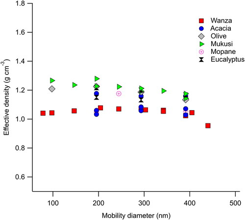
Our ${\rho }_{\mathit{eff}}$ results are similar to a previous lab study that focused on peat burning under different burning temperatures (Sumlin et al. 2018). However, our values are consistently lower than the reported ${\rho }_{\mathit{eff}}$ of rice straw burning done by Zhai et al. (2017). This could potentially be due to the presence of a larger fraction of inorganic components (nitrate, sulfate, chloride, and potassium) in the aerosol sample studied in Zhai et al. (2017). In addition, this study and a study by Sumlin et al. (2018) did not see a reasonable size-dependence of the ${\rho }_{\mathit{eff}},$ whereas Zhai et al. (2017) found larger ${\rho }_{\mathit{eff}}$ as the size increased. Values reported by Sumlin et al. (2018) and our study are lower than the ${\rho }_{\mathit{eff}}$ measured in the ambient environment (Qiao et al. 2018; McMurry et al. 2002), potentially due to a difference in the chemical composition of the aerosol. Besides comparing biomass burning studies in the laboratory and the field, we also compared the effective density estimated in this study with other examples of smoldering combustion, such as cigarette and marijuana smoke particles. Johnson et al. (2014) found that cigarette smoke particles have a spherical morphology with an average effective density of (1.18 ± 0.11) g cm⁻³. Another study by Graves et al. (2020) showed that effective densities of tobacco and marijuana smoke particles are independent of particle size above 150 nm, with effective densities of (0.99 ± 0.1) g cm⁻³ for tobacco and (0.90 ± 0.09) g cm⁻³ for marijuana. These values are also within the range (1.13 ± 0.07) g cm⁻³ of the values found in this study.

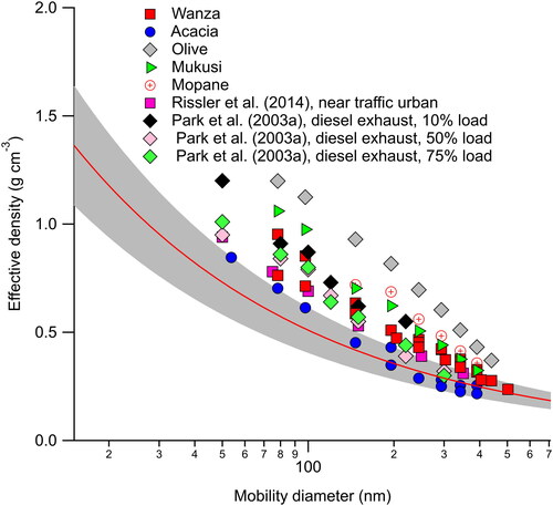
Unlike the ${\rho }_{\mathit{eff}}$ for the smoldering-dominated aerosol, the ${\rho }_{\mathit{eff}}$ of flaming-dominated aerosol (MCE > 0.95) shows strong particle size dependence, with a significant decrease in ${\rho }_{\mathit{eff}}$ with increasing mobility diameter, as shown in Figure 4. Although the general trend of ${\rho }_{\mathit{eff}}$ with mobility diameter was similar, there was clearly a fuel dependency for ${\rho }_{\mathit{eff}},$ with olive consistently higher compared to other fuels even under similar burn conditions (i.e., close MCE values for all the fuels present in Figure 4). This conclusion is corroborated by repeated burns of the same fuel (wanza and acacia), which produces nearly identical values of ${\rho }_{\mathit{eff}}.$ Since flaming combustion is dominated by black carbon emissions (Pokhrel et al. 2016; Stockwell et al. 2014) and potentially smaller size black carbon aggregates are made up of fewer primary spherules resulting in larger ${\rho }_{\mathit{eff}}$ for smaller size particles. In other words, smaller particles have structures that are more compact and closer to a sphere. As the particle size increases, the ${\rho }_{\mathit{eff}}$ decreases, approaching ∼0.3 g cm⁻³ for 450 nm size indicating the fractal nature of freshly emitted black carbon dominated aerosol. We compared the variation of ${\rho }_{\mathit{eff}}$ with d_m for the flaming-dominated aerosol in this study with the universal relation of the variation of ${\rho }_{\mathit{eff}}$ with d_m proposed by Olfert and Rogak (2019) based on the thermally denuded fresh soot emitted from the different kinds of ignition engines using different fuels. The red line and the shaded region in Figure 4 show the best fit line and the one standard deviation of the residuals proposed by the Olfert and Rogak (2019). As expected, the ${\rho }_{\mathit{eff}}$ values estimated in this study are significantly larger than the ${\rho }_{\mathit{eff}}$ values in Olfert and Rogak (2019) because they used bare soot, where volatile material has already evaporated. As discussed in section 2.5, some of this deviation could be due to presence of q > +1 charge, but does not totally explain the deviation observed in this study. The impact of q > +1 charge on ${\rho }_{\mathit{eff}}$ is at a maximum at 150 nm and smaller at particle size smaller and larger than 150 nm (Radney and Zangmeister 2016). However, we observed the largest deviation at smaller size and the deviation gradually decreases as particle size increases which could potentially be due to impact of co-emitted volatile materials along with BC particles. The presence of volatile material would increase the effective density of bare soot because volatile material fills the voids in the soot, resulting in the increase of the particle mass without a significant impact on its mobility diameter. Since we did not denude the particles in this study and the co-emitted organic aerosol produced during combustion is impacting the ${\rho }_{\mathit{eff}}$_, the resulting q_eff values are significantly larger than bare engine soot particles. Like our result, the ${\rho }_{\mathit{eff}}$ of diesel exhaust (Park et al. 2003a) and near traffic urban environment aerosol particles (Rissler et al. 2014) have significantly larger ${\rho }_{\mathit{eff}}$ than the values proposed by Olfert and Rogak (2019), potentially due to presence of volatile materials.

Figure 4. The effective density of freshly emitted flaming-dominated aerosol as a function of mobility diameter. Different colors and symbols represent different fuels, as indicated in the legend. Measurements of diesel exhaust at different loads (Park et al. 2003a) and near traffic urban environments (Rissler et al. 2014) are also present as a function of mobility diameter. The solid red line is the best fit line of effective density with mobility diameter proposed by Olfert and Rogak (2019) for freshly emitted thermally denuded soot with one standard deviation of residuals represented by shaded region. The data for the figure is provided in Table S3.

The differences in ${\rho }_{\mathit{eff}}$ between this study and those proposed by Olfert and Rogak (2019) show a size dependency, with relatively large differences at smaller sizes. For mobility diameters larger than 200 nm, our ${\rho }_{\mathit{eff}}$ values are close to the proposed values. This deviation is also expected, as there are a number of studies which show that the mass fraction of volatile material shows a power law relationship with the mobility diameter since there is a larger organic mass fraction at smaller size particles (Dickau et al. 2016; Graves et al. 2015; Ristimäki et al. 2007). Due to the presence of a larger fraction of volatile material (in our case potentially an organic aerosol) in smaller size particles, the deviation in ${\rho }_{\mathit{eff}}$ from bare soot results is larger for smaller particles.

The ${\rho }_{\mathit{eff}}$ for individual sizes, list of fuels, and corresponding MCE of the burns are presented in Table S3.

3.3. Dependence of mass mobility exponent on burning condition

The relationship between the mass mobility exponent and burning conditions was explored by the power-law relation between particle mass and the mobility diameter using Equation (4)(4) $$m_p=C{d}_m^{D_{fm}}$$(4) . Mass mobility exponent ($D_{fm}$) is calculated as a slope of the log-log plot of particle mass as a function of mobility diameter. An example of mass mobility exponent calculation for flaming and smoldering burns for wanza is provided in Figure S3 (SI). Depending on the burning conditions, the calculated $D_{fm}$ ranges from a maximum of 3.06 (±0.04) to a minimum of 2.15 (±0.10) for smoldering-dominated and flaming-dominated burns, respectively, with the number inside the parenthesis representing one standard deviation of the slope of an unweighted fit of the log-log plot of particle mass as a function of mobility diameter. The $D_{fm}$ values for each burn are provided in Table S4 (SI). The impact of burning conditions on $D_{fm}$ is explored by plotting $D_{fm}$ as a function of MCE for different burning conditions, as shown in Figure 5. The nature of the variation of $D_{fm}$ with MCE is best described by the Hill equation with maximum and minimum asymptotes of 2.97 ± 0.05 and 2.26 ± 0.05, respectively. The outlier at MCE ∼0.97 is omitted during the fitting of the Hill equation. The unweighted fitting line gives the continuum of $D_{fm}$ with values of ∼3 for MCE ≤ 0.92 then the $D_{fm}$ decreases sharply with MCE and ultimately remains independent as MCE > 0.95 with the $D_{fm}$ reaching the minimum asymptote. The maximum asymptote of (2.97 ± 0.05) indicates that the particles emitted during burns with MCE ≤ 0.92 are homogeneous spheres having mass mobility exponents of ∼3, which is consistent with the brown carbon emitted during smoldering peat burning in a previous study (Sumlin et al. 2018). Furthermore, the fitting coefficient base represents the minimum asymptote with a value of 2.26 ± 0.05, indicating that particles emitted during burns with MCE > 0.95 are non-spherical with mass mobility exponents similar to the previously studied externally mixed BC and diesel exhaust particles, with $D_{fm}$ ranging from 2.3 to 2.41 (Wu et al. 2019; Rissler et al. 2014; Maricq and Xu 2004; Park et al. 2003a, Park, Kittelson, and McMurry 2004). However, the minimum asymptote value found in this study is lower than the value ($D_{fm}$ = 2.48) proposed by Olfert and Rogak (2019) in their recent review article, but the variation in the literature is wide.

Figure 5. Mass mobility exponent as a function of modified combustion efficiency. The box and whisker plot shows the effective density of 200 nm size particles at three different regimes shown at right axis. The box top and bottom showing inter quartile range and whisker showing 95^th and 5^th percentile; central line shows the median value. Data points are given in Table S4.

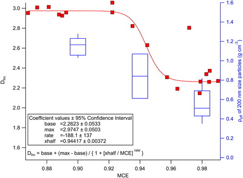
The relationship of $D_{fm}$ with MCE shows three distinct regimes. The first is a spherical particle regime (with characteristic $D_{fm}$ values of ∼3) where $D_{fm}$ is independent of the MCE but bounded by an MCE with an upper limit of ∼0.92. Even though an MCE of 0.9 is characterized as having equal portions of flaming and smoldering emissions, the particle morphology for MCE ≤ 0.92 shows similar $D_{fm}$ as the purely smoldering burn. The second regime is a transition regime, where $D_{fm}$ shows a strong dependency on the MCE and the particles emitted during these conditions (0.92 < MCE < 0.95) show a fractal nature with highly variable $D_{fm}$ values ranging from 2.3 <$D_{fm}<$3. The third regime, which we call the fractal regime, is where the $D_{fm}$ is ∼2.26 and is independent of the MCE of the burn, but bounded by the lower limit of an MCE of ∼0.96. Figure 5 also shows the box and whisker plot of effective density of 200 nm particles within the three different regimes. Since effective density shows size dependency at the transition and the fractal regimes, we reported 200 nm size particles as a representative case. As evident from Figure 5, the fractal and the spherical regimes have a very narrow range of effective densities regardless of fuel type whereas for transition regime, the variation is large for both effective density and $D_{fm}$ values. A literature review by Sorensen (2011) concluded that the $D_{fm}$ is 2.17 ± 0.1 for a diffusion-limited cluster aggregate (DLCA) with fractal dimension of 1.78 and pre-factor of 1.3. The $D_{fm}$ value for DLCA proposed by Sorensen (2011) compares well with the $D_{fm}$ for the fractal regime (2.26) found in this study. This fact suggests that the particles emitted during flaming-dominated burns have similar morphology as DLCA. Previous studies using scanning electron microscopy images found fractal dimension of soot aggregates emitted from wildfires to be in the range of 1.8-1.92 (Chakrabarty et al. 2014; China et al. 2013).

From the climate perspective, estimation of refractive indices (real and imaginary parts) of aerosol is the most important quantity to accurately estimate the aerosol radiative forcing. The optical closure method is the most common way to estimate the refractive indices of aerosol in the atmospheric science community (Sarpong et al. 2020; Radney and Zangmeister 2018; Saleh et al. 2014, 2016, 2018; Saliba et al. 2016; Mack et al. 2010), where optical properties estimated from the model are manually iterated until measured and estimated values match. For refractive indices calculations, the most commonly used approach is the Mie theory based model (Bohren and Huffman 1983) which treats aerosol particles as homogeneous spheres. However, there is signficant amount of evidence that shows that freshly emitted aerosol are fractal in nature (Chakrabarty et al. 2007, 2014; Bond et al. 2013; China et al. 2013; Sorensen 2001) and to accurately estimate their optical properties we must rely on a model which accounts for the fractal nature of aerosol, such as the Rayleigh–Debye–Gans (RDG) approximation (Liu et al. 2015; Chakrabarty et al. 2007). The relationship between $D_{fm}$ and MCE may not be directly applicable for RDG approximation calculation because use of RDG approximation requires additional parameters, such as the monomer diameter, the radius of gyration, and the fractal pre-factor. However, the proposed parameterization of $D_{fm}$ with the MCE will provide a critical tool to access whether the application of Mie-based calculations are appropriate or not based on the MCE calculation alone, even without aerosol morphology information.

4. Conclusions

In this study, we examined the physical and morphological properties of aerosol emitted from six different types of hardwood fuels native to sub-Saharan Africa under controlled laboratory burning conditions. It was found that flaming-dominated burning (MCE > 0.95) produced mostly ultrafine particles with GMD < 40 nm, whereas smoldering-dominated burning (MCE < 0.9) produced ultrafine and fine mode particles with GMD of ∼80 nm. The ${\rho }_{\mathit{eff}}$ of aerosol emitted during smoldering-dominated burns did not show a size dependency. Even though ${\rho }_{\mathit{eff}}$ showed a fuel dependency with consistently lower ${\rho }_{\mathit{eff}}$ values for some fuels, the variation was within 20% with ranges of ${\rho }_{\mathit{eff}}$ between (1.03 ± 0.05) g cm⁻³ to (1.21 ± 0.02) g cm⁻³. The mass mobility exponent ∼3 (2.97 ± 0.05) indicates that aerosol emitted during smoldering-dominated emissions were homogeneous spheres without internal voids; consistent with the organic carbon emitted during smoldering peat burning in a previous study (Sumlin et al. 2018).

Unlike smoldering-dominated burns, ${\rho }_{\mathit{eff}}$ of aerosol emitted during flaming-dominated burns showed a size-dependence, with a decrease in ${\rho }_{\mathit{eff}}$ as mobility diameter increased. The ${\rho }_{\mathit{eff}}$ decreased from (0.94 ± 0.21) g cm⁻³ at a mobility diameter of 80 nm to (0.31 ± 0.07) g cm⁻³ at a mobility diameter of 400 nm, indicating the fractal nature of the freshly emitted aerosol. The ${\rho }_{\mathit{eff}}$ of freshly emitted BB aerosol from flaming-dominated burns showed values consistent with the ${\rho }_{\mathit{eff}}$ of diesel exhaust particles under different loads (Park et al. 2003a) and with the near traffic urban environment aerosol (Rissler et al. 2014). The mass mobility exponent of (2.26 ± 0.05) for aerosol emitted during flaming-dominated emissions were commensurate with previously studied externally mixed BC and diesel exhaust particles. The relationship of $D_{fm}$ with MCE shows three distinct regimes, which we define as the spherical particle, transition, and fractal regime. The spherical particle regime shows $D_{fm}$ values of ∼3 and is independent of MCE, the transition regime shows the $D_{fm}$ is highly sensitive to the MCE, and the fractal regime is also independent of MCE and has $D_{fm}$ values similar to freshly emitted soot particles. Furthermore, we proposed a relationship between mass mobility exponent and MCE that can serve as a tool to assess whether the application of Mie theory-based calculations is justifiable or not.

Acknowledgments

We also acknowledge the help from Dr. Gizaw Mengistu Tsidu of Botswana International University of Science and Technology for providing wood samples from Botswana.

Additional information

Funding

This work is supported by NSF Grant # AGS1831013. JG acknowledges the partial supported by Department of Education under the Title III HBGI grant. Any opinions, findings, and conclusions or recommendations expressed in this material are those of the author(s) and do not necessarily reflect the views of Department of Education.

References

- Bohren, C. F., and D. R. Huffman. 1983. Absorption and scattering of light by small particles. New York: John Wiley Sons.
- Bond, T. C., S. J. Doherty, D. W. Fahey, P. M. Forster, T. Berntsen, B. J. Deangelo, M. G. Flanner, S. Ghan, B. Kärcher, D. Koch, et al. 2013. Bounding the role of black carbon in the climate system: A scientific assessment. J. Geophys. Res. Atmos. 118 (11):5380–552. doi:https://doi.org/10.1002/jgrd.50171.
- Bond, T. C., D. G. Streets, K. F. Yarber, S. M. Nelson, J. H. Woo, and Z. Klimont. 2004. A technology-based global inventory of black and organic carbon emissions from combustion. J. Geophys. Res 109:D14203.
- Brown, H., X. Liu, Y. Feng, Y. Jiang, M. Wu, Z. Lu, C. Wu, S. Murphy, and R. Pokhrel. 2018. Radiative effect and climate impacts of brown carbon with the community atmosphere model (CAM5). Atmos. Chem. Phys. 18 (24):17745–68. doi:https://doi.org/10.5194/acp-18-17745-2018.
- Cappa, C. D., T. B. Onasch, P. Massoli, D. R. Worsnop, T. S. Bates, E. S. Cross, P. Davidovits, J. Hakala, K. L. Hayden, B. T. Jobson, et al. 2012. Radiative absorption enhancements due to the mixing state of atmospheric black carbon. Science (80-.) 337 (6098):1078–81. doi:https://doi.org/10.1126/science.1223447.
- Carrico, C. M., A. J. Prenni, S. M. Kreidenweis, E. J. T. Levin, C. S. Mccluskey, P. J. DeMott, G. R. Mcmeeking, S. Nakao, C. E. Stockwell, and R. J. Yokelson. 2016. Rapidly evolving ultrafine and fine mode biomass smoke physical properties: Comparing laboratory and field results. J. Geophys. Res. Atmos. 121 (10):5750–68. doi:https://doi.org/10.1002/2015JD024389.
- Chakrabarty, R. K., N. D. Beres, H. Moosmüller, S. China, C. Mazzoleni, M. K. Dubey, L. Liu, and M. I. Mishchenko. 2014. Soot superaggregates from flaming wildfires and their direct radiative forcing. Sci. Rep 4:1–9.
- Chakrabarty, R. K., H. Moosmüller, W. P. Arnott, M. A. Garro, J. G. Slowik, E. S. Cross, J. H. Han, P. Davidovits, T. B. Onasch, and D. R. Worsnop. 2007. Light scattering and absorption by fractal-like carbonaceous chain aggregates: Comparison of theories and experiment. Appl Opt. 46 (28):6990–7006. doi:https://doi.org/10.1364/ao.46.006990.
- China, S., C. Mazzoleni, K. Gorkowski, A. C. Aiken, and M. K. Dubey. 2013. Morphology and mixing state of individual freshly emitted wildfire carbonaceous particles. Nat. Commun. 4 (2122).
- Christian, T. J., B. Kleiss, R. J. Yokelson, R. Holzinger, P. J. Crutzen, W. M. Hao, B. H. Saharjo, and D. E. Ward. 2003. Comprehensive laboratory measurements of biomass-burning emissions: 1. Emissions from Indonesian, African, and other fuels. J. Geophys. Res. 108 (D23): 4719 .
- Corbin, J. C., H. Czech, D. Massabò, F. B. de Mongeot, G. Jakobi, F. Liu, P. Lobo, C. Mennucci, A. A. Mensah, J. Orasche, et al. 2019. Infrared-absorbing carbonaceous tar can dominate light absorption by marine-engine exhaust. Npj Clim. Atmos. Sci. 2 (1).
- DeCarlo, P. F., J. G. Slowik, D. R. Worsnop, P. Davidovits, and J. L. Jimenez. 2004. Particle morphology and density characterization by combined mobility and aerodynamic diameter measurements. Part 2: Application to combustion-generated soot aerosols as a function of fuel equivalence ratio. Aerosol Sci. Technol. 38 (12):1185–205. doi:https://doi.org/10.1080/027868290903907.
- Dickau, M., J. Olfert, M. E. J. Stettler, A. Boies, A. Momenimovahed, K. Thomson, G. Smallwood, and M. Johnson. 2016. Methodology for quantifying the volatile mixing state of an aerosol. Aerosol Sci. Technol. 50 (8):759–72. doi:https://doi.org/10.1080/02786826.2016.1185509.
- Flowers, B. a., M. K. Dubey, C. Mazzoleni, E. a Stone, J. J. Schauer, S. W. Kim, and S. C. Yoon. 2010. Optical-chemical-microphysical relationships and closure studies for mixed carbonaceous aerosols observed at Jeju Island; 3-laser photoacoustic spectrometer, particle sizing, and filter analysis. Atmos. Chem. Phys. 10 (21):10387–98.
- Girotto, G.,. S. China, J. Bhandari, K. Gorkowski, B. V. Scarnato, T. Capek, A. Marinoni, D. P. Veghte, G. Kulkarni, A. C. Aiken, et al. 2018. Fractal-like Tar Ball Aggregates from Wildfire Smoke. Environ. Sci. Technol. Lett. 5 (6):360–5. doi:https://doi.org/10.1021/acs.estlett.8b00229.
- Gkatzelis, G. I., D. K. Papanastasiou, K. Florou, C. Kaltsonoudis, E. Louvaris, and S. N. Pandis. 2016. Measurement of nonvolatile particle number size distribution. Atmos. Meas. Tech. 9 (1):103–14. doi:https://doi.org/10.5194/amt-9-103-2016.
- Graves, B. M., T. J. Johnson, R. T. Nishida, R. P. Dias, B. Savareear, J. J. Harynuk, M. Kazemimanesh, J. S. Olfert, and A. M. Boies. 2020. Comprehensive characterization of mainstream marijuana and tobacco smoke. Sci. Rep. 10 (1):1–12.
- Graves, B., J. Olfert, B. Patychuk, R. Dastanpour, and S. Rogak. 2015. Characterization of particulate matter morphology and volatility from a compression-ignition natural-gas direct-injection engine. Aerosol Sci. Technol. 49 (8):589–98. doi:https://doi.org/10.1080/02786826.2015.1050482.
- IPCC2013. Anthropogenic and Natural Radiative Forcing, Climate Change 2013: The Physical Science Basis, Contribution of Working Group I to the Fifth Assessment Report of the Intergovernmental Panel on Climate Change, 659–740.
- Jacobson, M. Z. 2001. Strong radiative heating due to the mixing state of black carbon in atmospheric aerosols. Nature 409 (6821):695–7. doi:https://doi.org/10.1038/35055518.
- Johnson, T. J., J. S. Olfert, R. Cabot, C. Treacy, C. U. Yurteri, C. Dickens, J. McAughey, and J. P. R. Symonds. 2014. Steady-state measurement of the effective particle density of cigarette smoke. J. Aerosol Sci 75:9–16. doi:https://doi.org/10.1016/j.jaerosci.2014.04.006.
- Katrib, Y., S. T. Martin, Y. Rudich, P. Davidovits, J. T. Jayne, and D. R. Worsnop. 2005. Density changes of aerosol particles as a result of chemical reaction. Atmos. Chem. Phys. 5 (1):275–91. doi:https://doi.org/10.5194/acp-5-275-2005.
- Kirchstetter, T. W., and T. L. Thatcher. 2012. Contribution of organic carbon to wood smoke particulate matter absorption of solar radiation. Atmos. Chem. Phys. 12 (14):6067–72. doi:https://doi.org/10.5194/acp-12-6067-2012.
- Kumar, N. K., J. C. Corbin, E. A. Bruns, D. Massabó, J. G. Slowik, L. Drinovec, G. Močnik, P. Prati, A. Vlachou, U. Baltensperger, et al. 2018. Production of particulate brown carbon during atmospheric aging of wood-burning emissions. Atmos. Chem. Phys. 18 (24):17843–61. doi:https://doi.org/10.5194/acp-18-17843-2018.
- Lack, D. A., J. M. Langridge, R. Bahreini, C. D. Cappa, a M. Middlebrook, and J. P. Schwarz. 2012. Brown carbon and internal mixing in biomass burning particles. Proc. Natl. Acad. Sci. USA. 109 (37):14802–7. doi:https://doi.org/10.1073/pnas.1206575109.
- Laskin, A., J. Laskin, and S. a Nizkorodov. 2015. Chemistry of atmospheric brown carbon. Chem. Rev. 115 (10):4335–82. doi:https://doi.org/10.1021/cr5006167.
- Li, C., Y. Hu, J. Chen, Z. Ma, X. Ye, X. Yang, L. Wang, X. Wang, and A. Mellouki. 2016. Physiochemical properties of carbonaceous aerosol from agricultural residue burning: Density, volatility, and hygroscopicity. Atmos. Environ 140:94–105.
- Li, C., Z. Ma, J. Chen, X. Wang, X. Ye, L. Wang, X. Yang, H. Kan, D. J. Donaldson, and A. Mellouki. 2015. Evolution of biomass burning smoke particles in the dark. Atmos. Environ 120:244–52. doi:https://doi.org/10.1016/j.atmosenv.2015.09.003.
- Liu, X., R. C. Easter, S. J. Ghan, R. Zaveri, P. Rasch, X. Shi, J. F. Lamarque, A. Gettelman, H. Morrison, F. Vitt, et al. 2012. Toward a minimal representation of aerosols in climate models: Description and evaluation in the Community Atmosphere Model CAM5. Geosci. Model Dev. 5 (3):709–39.
- Liu, B. Y. H., and D. Y. H. Pui. 1974. A submicron aerosol standard and the primary, absolute calibration of the condensation nuclei counter. J. Colloid Interface Sci. 47 (1):155–71. doi:https://doi.org/10.1016/0021-9797(74)90090-3.
- Liu, D., J. W. Taylor, D. E. Young, M. J. Flynn, H. Coe, and J. D. Allan. 2015. The effect of complex black carbon microphysics on the determination of the optical properties of brown carbon. Geophys. Res. Lett. 42 (2):613–9. doi:https://doi.org/10.1002/2014GL062443.
- Mack, L. a., E. J. T. Levin, S. M. Kreidenweis, D. Obrist, H. Moosmüller, K. a Lewis, W. P. Arnott, G. R. McMeeking, a P. Sullivan, C. E. Wold, et al. 2010. Optical closure experiments for biomass smoke aerosols. Atmos. Chem. Phys. 10 (18):9017–26. doi:https://doi.org/10.5194/acp-10-9017-2010.
- Maricq, M. M., and N. Xu. 2004. The effective density and fractal dimension of soot particles from premixed flames and motor vehicle exhaust. J. Aerosol Sci. 35 (10):1251–74. doi:https://doi.org/10.1016/j.jaerosci.2004.05.002.
- McMeeking, G. R., E. Fortner, T. B. Onasch, J. W. Taylor, M. Flynn, H. Coe, and S. M. Kreidenweis. 2014. Impacts of nonrefractory material on light absorption by aerosols emitted from biomass burning. J. Geophys. Res. Atmos. 119:12272–86.
- McMurry, P. H., X. Wang, K. Park, and K. Ehara. 2002. The relationship between mass and mobility for atmospheric particles: A new technique for measuring particle density. Aerosol Sci. Technol. 36 (2):227–38. doi:https://doi.org/10.1080/027868202753504083.
- Olfert, J. S., M. Dickau, A. Momenimovahed, M. Saffaripour, K. Thomson, G. Smallwood, M. E. J. Stettler, A. Boies, Y. Sevcenco, A. Crayford, et al. 2017. Effective density and volatility of particles sampled from a helicopter gas turbine engine. Aerosol Sci. Technol. 51 (6):704–14. doi:https://doi.org/10.1080/02786826.2017.1292346.
- Olfert, J., and S. Rogak. 2019. Universal relations between soot effective density and primary particle size for common combustion sources. Aerosol Sci. Technol. 53 (5):485–92. doi:https://doi.org/10.1080/02786826.2019.1577949.
- Pagels, J., A. F. Khalizov, P. H. McMurry, and R. Y. Zhang. 2009. Processing of soot by controlled sulphuric acid and water condensation mass and mobility relationship. Aerosol Sci. Technol. 43 (7):629–40. doi:https://doi.org/10.1080/02786820902810685.
- Park, K., F. Cao, D. B. Kittelson, and P. H. McMurry. 2003a. Relationship between particle mass and mobility for diesel exhaust particles. Environ. Sci. Technol. 37 (3):577–83. doi:https://doi.org/10.1021/es025960v.
- Park, K., D. B. Kittelson, and P. H. McMurry. 2003b. A closure study of aerosol mass concentration measurements: Comparison of values obtained with filters and by direct measurements of mass distributions. Atmos. Environ. 37 (9/10):1223–30.
- Park, K., D. B. Kittelson, and P. H. McMurry. 2004. Structural properties of diesel exhaust particles measured by Transmission Electron Microscopy (TEM): Relationships to particle mass and mobility. Aerosol Sci. Technol. 38 (9):881–9.
- Pokhrel, R. P., E. R. Beamesderfer, N. L. Wagner, J. M. Langridge, D. A. Lack, T. Jayarathne, E. A. Stone, C. E. Stockwell, R. J. Yokelson, and S. M. Murphy. 2017. Relative importance of black carbon, brown carbon, and absorption enhancement from clear coatings in biomass burning emissions. Atmos. Chem. Phys. 17 (8):5063–78. doi:https://doi.org/10.5194/acp-17-5063-2017.
- Pokhrel, R. P., N. L. Wagner, J. M. Langridge, D. A. Lack, T. Jayarathne, E. A. Stone, C. E. Stockwell, R. J. Yokelson, and S. M. Murphy. 2016. Parameterization of single-scattering albedo (SSA) and absorption Ångström exponent (AAE) with EC/OC for aerosol emissions from biomass burning. Atmos. Chem. Phys. 16 (15):9549–61.
- Qiao, K., Z. Wu, X. Pei, Q. Liu, D. Shang, J. Zheng, Z. Du, W. Zhu, Y. Wu, S. Lou, et al. 2018. Size-resolved effective density of submicron particles during summertime in the rural atmosphere of Beijing. China. J. Environ. Sci. (China), 73:69–77. doi:https://doi.org/10.1016/j.jes.2018.01.012.
- Radney, J. G., and C. D. Zangmeister. 2016. Practical limitations of aerosol separation by a tandem differential mobility analyzer-aerosol particle mass analyzer. Aerosol Sci Technol. 50 (2):160–72. doi:https://doi.org/10.1080/02786826.2015.1136733.
- Radney, J. G., and C. D. Zangmeister. 2018. Comparing aerosol refractive indices retrieved from full distribution and size- and mass-selected measurements. J. Quant. Spectrosc. Radiat. Transf. 220:52–66. doi:https://doi.org/10.1016/j.jqsrt.2018.08.021.
- Rissler, J., E. Z. Nordin, A. C. Eriksson, P. T. Nilsson, M. Frosch, M. K. Sporre, A. Wierzbicka, B. Svenningsson, J. Löndahl, M. E. Messing, et al. 2014. Effective density and mixing state of aerosol particles in a near-traffic urban environment. Environ. Sci. Technol. 48 (11):6300–8. doi:https://doi.org/10.1021/es5000353.
- Ristimäki, J., K. Vaaraslahti, M. Lappi, and J. Keskinen. 2007. Hydrocarbon condensation in heavy-duty diesel exhaust. Environ. Sci. Technol. 41 (18):6397–402. doi:https://doi.org/10.1021/es0624319.
- Sakurai, H., K. Park, P. H. McMurry, D. D. Zarling, D. B. Kittelson, and P. J. Ziemann. 2003. Size-Dependent mixing characteristics of volatile and nonvolatile components in diesel exhaust aerosols. Environ. Sci. Technol. 37 (24):5487–95. doi:https://doi.org/10.1021/es034362t.
- Saleh, R., P. J. Adams, N. M. Donahue, and A. L. Robinson. 2016. The interplay between assumed morphology and the direct radiative effect of light-absorbing organic aerosol. Geophys. Res. Lett. 43 (16):8735–43. doi:https://doi.org/10.1002/2016GL069786.
- Saleh, R., Z. Cheng, and K. Atwi. 2018. The Brown-Black continuum of light-absorbing combustion aerosols. Environ. Sci. Technol. Lett. 5 (8):508–13. doi:https://doi.org/10.1021/acs.estlett.8b00305.
- Saleh, R., Hennigan, C. J. McMeeking, G. R. Chuang, W. K. Robinson, E. S. Coe, H. Donahue, N. M. Robinson, A. and L. 2013. Absorptivity of brown carbon in fresh and photo-chemically aged biomass-burning emissions. Atmos. Chem. Phys. 13 (15):7683–93. doi:https://doi.org/10.5194/acp-13-7683-2013.
- Saleh, R., E. S. Robinson, D. S. Tkacik, A. T. Ahern, S. Liu, A. C. Aiken, R. C. Sullivan, A. a Presto, M. K. Dubey, R. J. Yokelson, et al. 2014. Brownness of organics in aerosols from biomass burning linked to their black carbon content. Nature Geosci. 7 (9):647–50. doi:https://doi.org/10.1038/ngeo2220.
- Saliba, G., R. Subramanian, R. Saleh, A. T. Ahern, M. Eric, A. Tasoglou, R. C. Sullivan, J. Bhandari, A. L. Robinson, G. Saliba, et al. 2016. Optical properties of black carbon in cookstove emissions coated with secondary organic aerosols: Measurements and modeling. Aerosol Sci. Technol 50 (11):1264–76.
- Sarpong, E., D. Smith, R. Pokhrel, M. N. Fiddler, and S. Bililign. 2020. Refractive indices of biomass burning aerosols obtained from African biomass fuels using RDG approximation. Atmosp 11 (1):62.
- Smith, D. M., T. Cui, M. N. Fiddler, R. P. Pokhrel, J. D. Surratt, and S. Bililign. 2020a. Laboratory studies of fresh and aged biomass burning aerosols emitted from east African biomass fuels- Part 2: Chemical properties and characterization. Atmos. Chem. Phys. 20 (17):10169–91.
- Smith, D. M., M. N. Fiddler, R. P. Pokhrel, and S. Bililign. 2020b. Laboratory studies of fresh and aged biomass burning aerosols emitted from east African biomass fuels – Part 1: Optical properties. Atmos. Chem. Phys 20 (17):10149–68.
- Smith, D. M., M. N. Fiddler, K. G. Sexton, and S. Bililign. 2019. Construction and characterization of an indoor smog chamber for measuring the optical and physicochemical properties of aging biomass burning aerosols. Aerosol Air Qual. Res. 19 (3):467–83. doi:https://doi.org/10.4209/aaqr.2018.06.0243.
- Sorensen, C. M. 2001. Light scattering by fractal aggregates: A review. Aerosol Sci. Technol. 35 (2):648–87.
- Sorensen, C. M. 2011. The mobility of fractal aggregates: A review. Aerosol Sci. Technol. 45 (7):765–79. doi:https://doi.org/10.1080/02786826.2011.560909.
- Stockwell, C. E., R. J. Yokelson, S. M. Kreidenweis, A. L. Robinson, P. J. DeMott, R. C. Sullivan, J. Reardon, K. C. Ryan, D. W. T. Griffith, and L. Stevens. 2014. Trace gas emissions from combustion of peat, crop residue, biofuels, grasses, and other fuels: configuration and FTIR component of the fourth Fire Lab at Missoula Experiment (FLAME-4. Atmos. Chem. Phys. 14 (18):9727–54. ). doi:https://doi.org/10.5194/acp-14-9727-2014.
- Sumlin, B. J., C. R. Oxford, B. Seo, R. R. Pattison, B. J. Williams, and R. K. Chakrabarty. 2018. Density and homogeneous internal composition of primary brown carbon aerosol. Environ. Sci. Technol. 52 (7):3982–9. doi:https://doi.org/10.1021/acs.est.8b00093.
- Vakkari, V.,. V.-M. Kerminen, J. P. Beukes, P. Tiitta, P. G. van Zyl, M. Josipovic, A. D. Venter, K. Jaars, D. R. Worsnop, M. Kulmala, et al. 2014. Rapid change in biomass burning aerosols by atmospheric oxidation. Geophys. Res. Lett 41 (7):2644–51.,
- Wang, X., C. L. Heald, J. Liu, R. J. Weber, P. Campuzano-Jost, L. Jose, J. P. Schwarz, and A. E. Perring. 2018. Exploring the observational constraints on the simulation of brown carbon. Atmos. Chem. Phys. 18 (2):635–53. doi:https://doi.org/10.5194/acp-18-635-2018.
- Wu, Y., Y. Xia, R. Huang, Z. Deng, P. Tian, X. Xia, and R. Zhang. 2019. A study of the morphology and effective density of externally mixed black carbon aerosols in ambient air using a size-resolved single-particle soot photometer (SP2). Atmos. Meas. Technol. 12 (8):4347–59.
- Yokelson, R. J., D. E. Ward, R. A. Susott, J. Reardon, and D. W. T. Griffith. 1997. Emissions from smoldering combustion of biomass measured by open-path Fourier transform infrared spectroscopy. J. Geophys. Res. 102 (D15):18865–77. doi:https://doi.org/10.1029/97JD00852.
- Zhai, J., X. Lu, L. Li, Q. Zhang, C. Zhang, H. Chen, X. Yang, and J. Chen. 2017. Size-resolved chemical composition, effective density, and optical properties of biomass burning particles. Atmos. Chem. Phys. 17 (12):7481–93. doi:https://doi.org/10.5194/acp-17-7481-2017.
- Zhao, G., T. Tan, W. Zhao, S. Guo, P. Tian, and C. Zhao. 2019. A new parameterization scheme of the real part of the ambient aerosols refractive index. Atmos. Chem. Phys. 19 (20):12875–85. doi:https://doi.org/10.5194/acp-19-12875-2019.