Improved PM_2.5 concentration estimates from low-cost sensors using calibration models categorized by relative humidity

Abstract

Low-Cost Sensors (LCS) of fine particulate matter (PM_2.5) have been widely used to supplement regular air quality monitoring stations. However, the sensor output is impacted by environmental factors, especially relative humidity, and must be calibrated to yield estimates of concentrations. In this study, we evaluate the performance of a linear model and a generalized additive model (GAM) to calibrate the output of LCS PM_2.5 measurements in terms of different relative humidity levels. The method is based on co-located measurements from an LCS and a conventional reference monitor at two sites in an urban area in northern China. A stepwise variable selection of air pollutant concentrations and meteorological observations is used to select inputs to the model in order to improve the calibration ability. The results show that when relative humidity is below 75%, linear calibration of LCS PM_2.5 observations can output PM_2.5 mass concentrations close to the reference method with a correlation coefficient (R²) of 0.86. When relative humidity is above 75%, the GAM calibration model significantly outperforms the linear model, with an R² of approximately 0.83. Overall, the linear model exhibits good fitness in dry conditions, while the GAM captures PM_2.5 variations best in humid conditions. We conclude that low-cost PM_2.5 sensors are sensitive to relative humidity and that therefore condition-specific calibration methods need to be used to improve the quality of the data as well as to improve the match with reference measurements.

Copyright © 2021 American Association for Aerosol Research

EDITOR:

• Kihong Park

1. Introduction

Fine atmospheric particulate matter (PM_2.5, particulate matter with aerodynamic diameter ≤2.5 µm) containing complex chemical compounds, such as water-soluble ions, elemental carbon, organic carbon, and insoluble minerals, and with a large surface area to absorb toxic substances (Y. Zhang et al. 2016) pose a significant threat to human health (H. H. Zhang et al. 2018). Moreover, because of the small particle size, it can penetrate human respiratory tracts, alveoli, and even the blood stream through breathing, causing respiratory, stroke, lung, and cardiovascular diseases, as well as premature death (Apte et al. 2015; Brook et al. 2010; Pope et al. 2004; Shang et al. 2018; L. Yang et al. 2012). In the Global Burden of Disease (GBD) 2015 risks assessment, exposure to PM_2.5 was estimated to have caused 4.2 million deaths and was ranked as the fifth mortality risk factor worldwide (Cohen et al. 2017).

In order to reduce human PM_2.5 exposure and the associated health risks, government agencies have committed to strengthening air particulate matter (PM) pollution monitoring and formulating a series of pollutant emission reduction plans (Tian et al. 2019; Y. Wang et al. 2016; Q. Zhang et al. 2019). Conventionally, PM_2.5 concentrations are usually measured by fixed monitoring stations with advanced instrumentation, such as the U.S. EPA Federal Reference Methods (FRM) and Federal Equivalent Methods (FEM) (U.S. Environmental Protection Agency 2013). In China, the equivalent reference instruments usually include Tapered Element Oscillating Microbalance (TEOM) and Beta Attenuation Monitor (BAM) (Ministry of Ecology and Environment of China 2018). Scientific monitors ensure the quality of the measurements, but they are sparsely deployed in urban areas due to their high cost and necessary professional maintenance (Steinle, Reis, and Sabel 2013). An increasing number of studies show that the limited temporal and spatial resolution of regular monitoring sites are insufficient to capture the variability of atmospheric pollutants as well as detailed exposure concentrations. This makes it difficult to quantify human exposure for health risk assessments in epidemiological research (Apte et al. 2017; Ye et al. 2018). Therefore, Low-Cost Sensors (LCS) using optical PM_2.5 measurements rapidly became popular in order to supplement the deficiencies of conventional monitoring instruments. They are typically characterized by small size, lightweight, low power consumption, and easy maintenance (Badura et al. 2018). They offer promise for dense air quality monitoring networks, real-time pollution hotspot identification, and refined human exposure assessments (Gao, Cao, and Seto 2015; Pitchford et al. 2007; N. Zikova, Masiol, et al. 2017; Zusman et al. 2020).

However, the biggest limitation of low-cost light-scattering PM_2.5 sensors is that the accuracy and precision of the results are sensitive to particle concentrations, chemical composition, and meteorological conditions. Interference due to temperature and relative humidity (RH) is particularly common. The data needs to be calibrated and the data quality of the measurements is controversial (Liu et al. 2017; Woodall et al. 2017; Zheng et al. 2018; Nadezda Zikova, Hopke, et al. 2017). Even though LCS performance has been estimated in the laboratory under particular conditions (Sayahi et al. 2019a), concerns remain about their performance in real-world environments (Cordero, Borge, and Narros 2018; Li and Biswas 2017).

Field calibration is used to obtain the best possible estimates of PM_2.5 concentrations in ambient air, but getting accurate results can be particularly challenging under extreme meteorological conditions or during extreme pollution episodes. Previous studies have examined the performance of numerous field calibration models by comparing low-cost PM sensors to standard particle concentration measuring instruments. The most widely used model is linear regression, which assumes that there is a linear relationship between LCS data and research-grade instrument measurements (Jovasevic-Stojanovic et al. 2015; Nakayama et al. 2018). Relative humidity plays an important role in the calibration process as it leads to particle growth through moisture absorption as well as the formation of water droplets that can be detected as aerosols. Badura et al. (2019) suggested that temperature and relative humidity should be used as inputs to the linear model in order to improve the calibration performance. However, it is thought that the response of LCS to relative humidity is non-linear in Di Antonio et al. (2018), the PM_2.5 concentrations reported by the PMS1003 were found to increase exponentially with relative humidity up to 75% (Jayaratne et al. 2018). To address this problem, non-linear models, and machine learning techniques, have been applied in order to obtain a better match with measurements from reference instruments (Topalović et al. 2019; Y. Wang et al. 2019). Because the sensor response varies under different target humidity conditions, it is necessary to evaluate whether the same field calibration method is applicable in all cases (Kelly et al. 2017; Zusman et al. 2020). Few studies have comprehensively considered the accuracy and efficiency of humidity-specific calibration models.

Our study aims to explore the performance characteristics of field calibration methods using both a linear model and a Generalized Additive Model (GAM) for PMS5003 sensors’ PM_2.5 measurements under different relative humidity levels in a 37-day monitoring campaign. The GAM was used to capture non-linear associations of hourly concentrations of PM_2.5 measurements with potential impactors, which has been shown to perform well (Lee, Wang, and Yu 2019). Additional impactors, such as meteorological and gas pollutant parameters, were introduced in order to improve the performance of the calibration model.

2. Materials and methods

2.1. Measurements

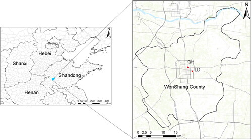
The field campaign was carried out from 11/01/2017 to 12/07/2017 during the heating season of northern China, which experiences high PM_2.5 mass concentrations. The monitoring sites (Figure 1), named as Lvdi (LD) and Quanhe (QH), were in Wenshang County, Shandong Province, China. The two sites were approximately 2 km apart and surrounded by similar land use types. They are both located in urban residential areas, close to major roadways, and were probably both impacted by coal combustion and traffic emissions. Therefore, we merged the original measurements of the two sites to a single dataset in order to carry out a single calibration model for both time series at once.

Figure 1. Map of Wenshang County, Shandong Province, China, with the triangles showing the two sites with co-located reference monitoring stations and LCS which are named Lvdi (LD) and Quanhe (QH), respectively, representing urban residential and traffic influenced environment.

In our study, a portable commercial measurement station (Figure 2) provided by Zhongke YunTian Environmental Protection Technology Company (located in Jining, China) was deployed at both the LD and QH sites. Each station consisted of a particulate matter monitoring module, gas pollutant monitoring modules, meteorological parameter sensors, a wireless communication module, a power supply, and a power management unit. Overall, an array of sensors was used to measure PM_2.5, carbon monoxide (CO), temperature, relative humidity, wind speed, and pressure. The sensor type of PM_2.5 measurements is PMS5003 (about USD 30), which was manufactured by Plantower, China. It is based on the light scattering of aerosols. The PMS5003 photodiode detector measures the intensity of scattered light after a laser beam passes through the air sample. This is used to estimate the equivalent grain size of particles, and the number of particles per unit volume by different particle diameters. The estimates are calculated using Mie theory as described on the website (http://www.plantower.com/). As with most sensors, the portable measurement station has no heating equipment at the inlet to remove water from the measurements and therefore relative humidity probably has an impact on particle refractive properties, and, thus, affects the optical information received by the sensors (Manikonda et al. 2016). Before field deployment, a trial operation of portable measurement station was implemented in which hourly data was collected for 10 days in order to ensure the efficiency and stability of every sensor, and no extra calibration was made due to the difference between laboratory and field conditions. During the monitoring period, the portable measurement stations were checked once a week to confirm normal operation and continuous data collection. The values were provided both raw PM_2.5 and ambient corrected PM_2.5 (Barkjohn et al. 2020; Tryner et al. 2020), the analysis in this study was based on the raw PM_2.5 concentrations reported by the PMS5003 without ambient corrections.

Figure 2. Left: Example of the monitoring airbox which contains an array of sensors measuring PM_2.5 (Plantower PMS5003), CO, temperature, relative humidity, wind speed, and pressure. Both are mounted to the rooftop of the building, where there are no specific source emissions from the surrounding area. Right: Internal view of the equipment box.

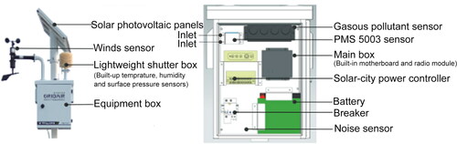
Each portable measurement station was deployed alongside a conventional instrument: The Met One Beta Attenuation Monitor (BAM) operating using the U.S. EPA Federal Equivalent Method (FEM) for continuous PM_2.5 monitoring. The instrument has a dryer at the inlet to remove water vapor, which minimizes the influence from relative humidity (Chung et al. 2001). The conventional instrument was operated and maintained by the Jining Ecological and Environmental Agency, and hourly values of PM_2.5, CO, nitrogen dioxide (NO₂), sulfur dioxide (NO₂), ozone (O₃), temperature, relative humidity, wind speed, and pressure were available. Note that in the following section the terms ${\mathrm{PM}}_{2.5}^{\mathrm{Ref}},\mathrm{}{\mathrm{CO}}^{\mathrm{Ref}},\mathrm{}{{\mathrm{NO}}_2^{\mathrm{Ref}},{\mathrm{SO}}_2^{\mathrm{Ref}},{\mathrm{O}}_3^{\mathrm{Ref}},\mathrm{}\mathrm{T}}^{\mathrm{Ref}},$${\mathrm{RH}}^{\mathrm{Ref}},$ $\mathrm{}{\mathrm{WS}}^{\mathrm{Ref}},$ and$\mathrm{}{\mathrm{P}}^{\mathrm{Ref}}$ are used to represent the reference stations’ measured parameters of PM_2.5, CO, NO₂, SO₂, O₃, temperature, relative humidity, wind speed, and pressure, respectively. The terms ${\mathrm{PM}}_{2.5}^{\mathrm{LCS}},\mathrm{}{\mathrm{CO}}^{\mathrm{LCS}},{\mathrm{T}}^{\mathrm{LCS}},$${\mathrm{RH}}^{\mathrm{LCS}},$$\mathrm{}{\mathrm{WS}}^{\mathrm{LCS}},$ and$\mathrm{}{\mathrm{P}}^{\mathrm{LCS}}$ represent the LCS variables of PM_2.5, CO, temperature, relative humidity, wind speed, and pressure, respectively. LCS measurements were averaged to hourly values from one-minute resolution in order to match with the reference measurements. Hours with missing values were removed from the analysis, resulting in 87% data completeness.

2.2. Data analysis and LCS PM_2.5 calibration models

2.2.1. Data analysis

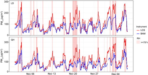
Our monitoring period experienced frequent elevated PM_2.5 concentrations as well as high relative humidity weather (Figure 3). Time series (Figure 3) of sensors and BAM PM_2.5 mass concentrations showed that peak PM_2.5 events corresponded to episodes with high relative humidity (≥75%). Jayaratne et al. (2018) found a marked increase of PM_2.5 concentrations reported by PMS1003 once relative humidity exceeded 75%. This happens when substances in the particles such as sodium chloride exceed their deliquescence point. The ratio of the PMS5003-reported PM_2.5 concentration to the dry TEOM-reported PM_2.5 concentration increased sharply for RH above about 74% (Tryner et al. 2020). Cruz and Pandis (2000) also report that sodium chloride and ammonium sulfate particles reached their deliquescence point when the relative humidity is above 75%. For substances with a deliquescence point, when the relative humidity exceeds the deliquescence point, the particulate matter will quickly absorb moisture, the scattering coefficient suddenly increases, and hygroscopic growth shows a significant jump with the relative humidity. Visual inspection of Figure S2 in the online SI shows that there is a difference in the characteristics of the measurements below and above an RH of approximately 75%. Above this threshold, the overestimation of LCS measurements in our field experiment increased rapidly with increasing RH (Figure S2a in the online SI). We therefore decided to separate the dataset into two groups according to whether the values of LCS relative humidity were below or above 75%. The first group corresponds to dry conditions and contained 1343 observations. The second group corresponds to humid conditions (${\mathrm{RH}}^{\mathrm{LCS}}$ values that are equal to or greater than 75%) and contained 207 data points.

Figure 3. Time series of hourly PM2_.5 mass concentrations measured by BAM and LCS along with relative humidity, measured between 1 November and 7 December 2017 at the two sites. The red shadow area represents the period of relative humidity measured by sensors as equal to or greater than 75%. (Upper: LD site; lower: QH site.)

2.2.2. Variables selection method for calibration models

Calibration models were performed using ${\mathrm{PM}}_{2.5}^{\mathrm{Ref}}$ as the dependent variable and ${\mathrm{PM}}_{2.5}^{\mathrm{LCS}}$ as the independent variable along with the additional calibration predictors shown in Table 2. The additional predictors were selected using a stepwise forward process, which began with an empty model and gradually added one variable at a time as an input to the linear model or GAM. In each step, the variable that contributes to the greatest improvement in the coefficient of determination (R²) was included (de Foy et al. 2018). The variable selection was carried out iteratively. With the increase of numbers of the input variables, the R² increased, however, the inclusion of reductant variables with low R² contributions would lead collinearity problems. By visual inspection, we can estimate the position of an inflection point in the curvature of R² vs. number of variables shown in Figure S5 in the online SI, and we use this to determine the optimal number of inputs to the model. The threshold at the inflection point was about 0.005 and 0.03 for dry and humid conditions, respectively (Figure S5 in the online SI). Therefore, for the model for dry conditions, as long as the new input variable contributed to an increase in R² of at least 0.005 it was retained in the list of model inputs, for humid conditions we used a threshold of 0.03. The difference arose mainly because there was much better agreement between the LCS and reference measurements during the dry conditions than during the humid conditions and will be discussed further in Section 3.2.

Table 2. List of calibration models developed in this study using linear and GAM calibration models under dry and humid conditions, along with input variables used for each model and corresponding statistical performance metrics.

Dry conditions	Formula	R²			RMSE (µg/m^3)
Uncalibrated measurements correlation	${PM}_{2.5}^{\mathit{Ref}}$∼${PM}_{2.5}^{\mathit{LCS}}$	0.82			81.39
Linear one variable	${PM}_{2.5}^{\mathit{Ref}}$∼f (${\widehat{PM}}_{2.5}^{\mathit{LCS}}$)	0.82			16.80
Linear three variables	${PM}_{2.5}^{\mathit{Ref}}$∼f (${\widehat{PM}}_{2.5}^{\mathit{LCS}}$+${\widehat{T}}^{\mathit{LCS}}$+${\widehat{RH}}^{\mathit{LCS}}$)	0.86			15.02
Uncalibrated measurements correlation	${PM}_{2.5}^{\mathit{Ref}}$∼${PM}_{2.5}^{\mathit{LCS}}$	0.82			81.39
GAM one variable	${PM}_{2.5}^{\mathit{Ref}}$∼s (${\widehat{PM}}_{2.5}^{\mathit{LCS}}$)	0.82			16.77
GAM four variables	${PM}_{2.5}^{\mathit{Ref}}$∼s (${\widehat{PM}}_{2.5}^{\mathit{LCS}}$+${\widehat{T}}^{\mathit{LCS}}$+${\widehat{RH}}^{\mathit{LCS}}$+${\widehat{CO}}^{\mathit{Ref}}$)	0.88			14.09
Humid conditions	Formula	R²			RMSE (µg/m^3)
Uncalibrated measurements correlation	${PM}_{2.5}^{\mathit{Ref}}$∼${PM}_{2.5}^{\mathit{LCS}}$	0.50			113.56
Linear one variable	${PM}_{2.5}^{\mathit{Ref}}$∼f (${\widehat{PM}}_{2.5}^{\mathit{LCS}}$)	0.50			31.28
Linear four variables	${PM}_{2.5}^{\mathit{Ref}}$∼f (${\widehat{PM}}_{2.5}^{\mathit{LCS}}$+${\widehat{WS}}^{\mathit{Ref}}$+${\widehat{RH}}^{\mathit{LCS}}$+${\widehat{CO}}^{\mathit{LCS}}$)	0.75			21.54
Uncalibrated measurements correlation	${PM}_{2.5}^{\mathit{Ref}}$∼${PM}_{2.5}^{\mathit{LCS}}$	0.50			113.33
GAM one variable	${PM}_{2.5}^{\mathit{Ref}}$∼s (${\widehat{PM}}_{2.5}^{\mathit{LCS}}$)	0.52			29.46
GAM four variables	${PM}_{2.5}^{\mathit{Ref}}$∼s (${\widehat{PM}}_{2.5}^{\mathit{LCS}}$+${\widehat{RH}}^{\mathit{LCS}}$+${\widehat{WS}}^{\mathit{LCS}}$+${\widehat{T}}^{\mathit{LCS}}$)	0.83			15.17

The predictors were normalized to obtain zero mean and unit standard deviation so as to reduce the effects of extreme observations. All available measurements were used as candidate inputs to the GAM in order to identify existing dependencies in the measurements. In the future, we could limit the candidate inputs to just the LCS measurements in order to develop an operational correction algorithm for the LCS product as was done for example in (Barkjohn et al. 2020).

2.2.3. Linear calibration based on reference measurements

The linear model was used to establish the relationships between the target variable and one or more predictors, which is one of the most widely used methods for calibrating LCS measurements. First, we derived the calibration formula by fitting a linear regression model to hourly LCS and co-located BAM PM_2.5 values. The equation is as follows: (1) $${\mathrm{PM}}_{2.5}^{\mathrm{Ref}}={\mathrm{\alpha }}_0+{\mathrm{\alpha }}_1{\times \widehat{\mathrm{PM}}}_{2.5}^{\mathrm{LCS}}+{\mathrm{\epsilon }}_1$$(1) where ${PM}_{2.5}^{\mathit{Ref}}$ (PM_2.5 mass concentrations measured by BAM) represents the dependent variable; ${\widehat{\mathrm{PM}}}_{2.5}^{\mathrm{LCS}}$ is the LCS PM_2.5 used as the predictor variable and normed to have zero mean and unit standard deviation; α₀ and α₁ are the intercept and slope of linear regression; ${\mathrm{\epsilon }}_1$ denotes the random residual.

The linear calibration model with stepwise forward selection of variables is an expansion of the linear regression model using the following equation: (2) $${\mathrm{PM}}_{2.5}^{\mathrm{Ref}}={\mathrm{\alpha }}_0+{\mathrm{\alpha }}_1\times \widehat{{\mathrm{x}}_1}+{\mathrm{\alpha }}_2\times \widehat{{\mathrm{x}}_2}+{\cdots +\mathrm{\alpha }}_{\mathrm{n}}\times \widehat{{\mathrm{x}}_{\mathrm{n}}}+{\mathrm{\epsilon }}_1$$(2) where n is the number of included predictors; $\widehat{{\mathrm{x}}_1}$ to $\widehat{{\mathrm{x}}_{\mathrm{n}}}$ are the normalized values of the predictors x₁ to x_n; and α₁…α_n are the regression coefficients corresponding to each predictor.

2.2.4. Gam calibration based on reference measurements

We tested the non-linear relationships of the PM_2.5 concentrations to several predictors by using the GAM (Hua et al. 2021) calibration method which is a nonparametric regression method. In order to obtain an optimal model, identical to the linear calibration model, we first input only ${\mathrm{PM}}_{2.5}^{\mathrm{LCS}}$ as a predictor, and then we included variables based on a stepwise forward selection algorithm. The smooth function can be described as (Eilers and Marx 1996; Wood and Augustin 2002): (3) $${\mathrm{PM}}_{2.5}^{\mathrm{Ref}}={\mathrm{\beta }}_0+{\mathrm{s}(\widehat{\mathrm{PM}}}_{2.5}^{\mathrm{LCS}})+{\mathrm{\epsilon }}_2$$(3) where β₀ is the intercept for GAM, ${\mathrm{s}(\widehat{\mathrm{PM}}}_{2.5}^{\mathrm{LCS}})\mathrm{}$ is the smooth function of normalized low-cost PM_2.5 sensors measurements, and ${\mathrm{\epsilon }}_2$ are the residuals. (4) $${\mathrm{PM}}_{2.5}^{\mathrm{Ref}}={\mathrm{\beta }}_0+\mathrm{s}\left(\widehat{{\mathrm{x}}_1}\right)+\mathrm{s}\left(\widehat{{\mathrm{x}}_2}\right)+\cdots +\mathrm{s}\left(\widehat{{\mathrm{x}}_{\mathrm{n}}}\right)+{\mathrm{\epsilon }}_2$$(4) where s(·) is the P-spline smoothing functions which optimize the fitting and control the smoothness through a penalty term (Eilers and Marx 1996), $s\left(\widehat{{\mathrm{x}}_1}\right)$ to $s\left(\widehat{{\mathrm{x}}_2}\right)$ are the smoothers which characterize the effects of the normalized x₁, x₂, and x_n on the reference PM_2.5 measurements, and n is the number of selected predictors.

2.3. Calibration performance metrics

The performance of calibration models was assessed using the coefficient of determination (R²) and root mean square error (RMSE) statistics. R² measures relationships between calibrated LCS and reference BAM PM_2.5 values. The value is between zero and one, and closer to one reflects better fitting quality. RMSE provides a measure for error between sensors and standard monitors measurements (Feenstra et al. 2019). The equations for R² and RMSE are as follows: (5) $$\text{Coefficient of determination}\left({\mathrm{R}}^2\right)\mathrm{}=1-\frac{{\sum }_{\mathrm{i}=1}^{\mathrm{n}}{({\mathrm{x}}_{\mathrm{i}}-\mathrm{}{\mathrm{y}}_{\mathrm{i}})}^2}{{\sum }_{\mathrm{i}=1}^{\mathrm{n}}{({\mathrm{y}}_{\text{i}}-\overline{y})}^2}$$(5) (6) $$\text{Root mean square error}\left(\mathrm{RMSE}\right)\mathrm{}=\sqrt{\frac{{\sum }_{\mathrm{i}=1}^{\mathrm{n}}{({\mathrm{x}}_{\mathrm{i}}-{\text{y}}_{\mathrm{i}})}^2}{\mathrm{n}}}$$(6) where x_i is the calibrated values of LCS PM_2.5, y_i is the PM_2.5 values measured by research-grade BAM,$\overline{y}$ is the average concentration of BAM PM_2.5, and n is the number of measurements.

Bootstrapping was used to estimate the uncertainty of the linear calibration model. The regression model was obtained 100 times using a randomly resampled dataset each time. When resampling the dataset, the data to be included were selected at random with replacement so that each dataset was of the same size as the original. The models were tested with 1-h to 24-h consecutive selections and found the results to be stable over time (Table S1). The uncertainty in the model coefficients was obtained from the variance of the 100 model simulations (de Foy and Schauer 2015).

Table 1. Statistical summary of measured parameters under dry and humid conditions. The parameters include PM_2.5, wind speed (WS), air temperature (T), relative humidity (RH), surface pressure (P) and carbon monoxide (CO), respectively, from BAM and LCS, and SO₂, NO₂, and O₃ from BAM.

Conditions	Parameters	Unit	Measurements from BAM			Measurements from LCS
			Mean	Median	Range	Mean	Median	Range
Dry conditions	PM2.5	µg/m^3	70.9	63.0	2.0–230.0	97.0	85.5	7.1 ∼ 335.6
	WS	m/s	1.6	1.5	0.0–6.0	0.6	0.5	0.0 ∼ 2.8
	T	°C	8.9	8.9	−4.5 to 23.8	8.1	8.1	−4.6 ∼ 22.9
	RH	%	47.1	47.0	18.0–72.0	48.0	47.5	16.4 ∼ 74.9
	P	hPa	1022	1022	1010–1036	1032	1032	1016 ∼ 1048
	CO	µg/m^3	1.1	1.1	0.2–2.6	0.5	0.5	0.0 ∼ 1.8
	SO2	µg/m^3	22.9	21.0	5.0–90.0	–	–	–
	NO2	µg/m^3	51.6	51.0	10.0–140.0	–	–	–
	O3	µg/m^3	39.2	32.0	2.0–136.0	–	–	–
Humid conditions	PM2.5	µg/m^3	101.8	99.0	39.0–223.0	186.0	191.9	71.9–325.9
	WS	m/s	1.2	1.2	0.0–3.1	0.3	0.1	0.0–1.4
	T	°C	5.8	5.2	−1.3 to 14.9	5.0	3.8	−1.9 to 13.7
	RH	%	62.8	64.0	34.0–83.0	82.2	81.3	75.1–95.8
	P	hPa	1021	1021	1012–1031	1030	1030	1018–1042
	CO	µg/m^3	1.4	1.4	0.6–2.8	0.7	0.7	0.2–1.6
	SO2	µg/m^3	18.8	17.0	3.0–45.0	–	–	–
	NO2	µg/m^3	60.9	59.0	22.0–106.0	–	–	–
	O3	µg/m^3	10.8	6.0	2.0–67.0	–	–	–

Data preprocessing, data analysis, linear model and GAM calculation, and model validation process were performed using the R environment (Version 3.6.3) (R Core Team 2019) with the “reshape,” “ggplot2,” “mgcv,” and “boot” packages.

3. Results and discussion

3.1. Time series analysis

The time series of hourly BAM and LCS PM_2.5 mass concentrations, along with LCS RH values at the LD and QH sites, can be seen in Figure 3. Other environmental factors reported by the BAM instrument at LD are also provided in Figure S1 in the online SI. It shows that LCS PM_2.5 values agree quite well (R² = 0.74) with BAM PM_2.5 measurements. The LCS PM_2.5 measurements somewhat overestimate and are sensitive to sudden peaks in values during the monitoring period, which was also found in a previous study in Salt Lake City, USA (Sayahi, Butterfield, and Kelly 2019b). Compared to the BAM, LCS overestimated PM_2.5 mass concentrations by a factor of about 1.4 in dry conditions and about 2.0 in humid conditions (Figure S2a in the online SI). The BAM instrument is using the sharp cyclone to remove particles larger than 2.5 µm. In contrast, the PMS5003 screened for PM_2.5 by estimating the particle size from light scattering. Based on Mie theory and assumptions of spherical particles and specific refractive index, the algorithm estimates the particle size from the amount of light of a known wavelength scattered at a fixed angle. The optical equivalent diameter of the particle sensor is usually calibrated using polystyrene standard particles and an assumed density of 1.5 g/cm³. Although the sensors were calibrated by Plantower using standard particles in the laboratory, these overestimation factors will be influenced by differences in real-world conditions as well as varying protocols from different manufacturers (Pawar and Sinha 2020). The methods used for distinguishing PM_2.5 from larger particles are different for each instrument and are a known source of discrepancy. However, there is no clear proxy to estimate the time-varying size of this effect and so, in this study, any systematic biases introduced in the measurements can only be accounted for at the same time as the other sources of error by the linear and GAM models.

The overestimated factors are similar to the results of (Sayahi, Butterfield, and Kelly 2019b), but are slightly greater in humid conditions. This is probably because the chemical composition of the aerosols in our study are different from those of Salt Lake City leading to changes in the instrument response as a function of relative humidity. In China, PM_2.5 contains high abundances of organic matter during haze events (An et al. 2019). Furthermore, the stagnant weather and rapid increase of RH enhance particle hygroscopic growth (Liu et al. 2011). In the Salt Lake area, particles are primarily composed of secondary inorganic aerosol, especially ammonium nitrate, which is mainly related to inversions (Kuprov et al. 2014). High RH during our study was therefore a likely cause of the LCS overestimation compared with the reference measurements. Compared to the high RH environment, PM_2.5 concentrations measured by LCS and BAM are more consistent in a lower RH environment. The correlation coefficient value is 0.91 (Figure S3 in the online SI), and is close to the results of (Sayahi, Butterfield, and Kelly 2019b).

The statistical summary of measured parameters is shown in Table 1. In dry and humid conditions, average LCS PM_2.5 concentrations are 97.0 µg/m³ and 186.0 µg/m³, while average BAM PM_2.5 concentrations are 70.9 µg/m³ and 101.8 µg/m³, respectively. Increasing RH drives particles hygroscopic growth, augments the PM_2.5 mass concentrations (An et al. 2019; Tie et al. 2017), affects the responses from the light scattering of sensors, results in a decrease of monitoring accuracy, and causes greater variation of PM_2.5 measurements of LCS (Yang Wang et al. 2015).

In light of the different degrees of response to the sensors due to different humidity conditions, the relationship between the independent variables and the dependent variable is more complicated, Figure S2a in the online SI shows that ${\mathrm{PM}}_{2.5}^{\mathrm{LCS}}$ exhibits a nonlinear response when relative humidity exceeds 75%. Therefore, we divided the observations into two groups based on RH values, and evaluated the applicability of linear and GAM calibration methods separately for each group. Distribution of PM_2.5 mass concentrations by BAM and LCS under dry and humid conditions is shown in Figure S4 in the online SI. The variance of LCS PM_2.5 measurements is higher than that of BAM in humid conditions. This is the main reason for the greater uncertainty of the calibration results, as well as for the lower calibration accuracy of humid conditions as opposed to dry conditions.

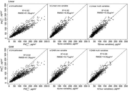
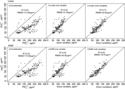
Figure 4. Comparison (a) uncalibrated PM_2.5 mass concentrations, (b) calibrated PM_2.5 values with linear model only included one variable, (c) calibrated PM_2.5 values with linear model included three variables, (d) uncalibrated PM_2.5 mass concentrations, (e) calibrated PM_2.5 values with GAM calibration only included one variable, and (f) calibrated PM_2.5 values with GAM calibration included four variables fitted to reference monitors hourly PM2_.5 mass concentrations in dry conditions. R² represents the regression coefficients between all LCS PM_2.5 measurements and reference BAM PM_2.5 values, and the line represents 1:1 fitting line.

3.2. Explanatory variables considered in calibration models

Figure S3 in the online SI shows the correlation coefficients (R) of all measured parameters in different relative humidity conditions. PM_2.5 measurements of LCS correlated very well with conventional monitors, demonstrating that the PMS5003 sensor is a useful tool for PM_2.5 monitoring. PM_2.5 was significantly positively correlated with relative humidity due to particle hygroscopic growth; droplets are easily detected by sensors and cause high overestimation in the measurements (Pawar and Sinha 2020). PM_2.5 was negatively correlated with wind speed, because in China haze episodes are usually accompanied by high humidity and stagnant weather (Sun et al. 2019). Wind speed can be an indirect factor in intensifying secondary conversion of gaseous pollutants and increasing moisture absorption of particulate matter. In addition, temperature might affect sensor performance and should be considered (Malings et al. 2020). PM_2.5 exhibits positive associations with CO, SO₂, and NO₂, which indicates that residential emissions, such as coal combustion and biomass burning for residential heating and cooking as well as transportation emissions have a large contribution to PM_2.5 pollution in the winter for the study area. The gas pollutants serve as indicators of different sources which have key impacts on PM_2.5 composition, and hence influence aerosol morphology and optical properties (Li et al. 2016).

Because there are high correlation coefficients between multiple predictors, the models run the risk of overfitting. This is especially the case if the parameters obtained by BAM and LCS monitoring are introduced at the same time. We therefore use a stepwise forward variable selection algorithm to screen the input variables. All variables in the candidate list are tested in the model individually. The predictor leading to the greatest increase in R² is added to the list of model inputs. This process is repeated so long as the R² is increased by 0.005 for the humid model and 0.03 for the dry model. This method not only controls the number of variables and reduces the model complexity, but also avoids introducing highly correlated explanatory variables, which improves model robustness. The increase in model R² as a function of the number of input variables is shown in Figure S5 in the online SI for the linear and GAM models under dry and humid conditions. Under dry conditions, when the number of input variables is greater than three, the increase of R² value tends to be low. Under humid conditions, when the number of variables is greater than four, the increase of R² value is low. The final variables selected are shown in Table 2. For the dry conditions, the linear model includes ${\mathrm{PM}}_{2.5}^{\mathrm{LCS}},$$\mathrm{}{\mathrm{T}}^{\mathrm{LCS}},$ and ${\mathrm{RH}}^{\mathrm{LCS}},$ and the GAM model includes ${\mathrm{PM}}_{2.5}^{\mathrm{LCS}},$$\mathrm{}{\mathrm{T}}^{\mathrm{LCS}},$ ${\mathrm{RH}}^{\mathrm{LCS}},$ and ${\mathrm{CO}}^{\mathrm{Ref}}.$ For the humid conditions, the linear model includes ${\mathrm{PM}}_{2.5}^{\mathrm{LCS}},$$\mathrm{}{\mathrm{WS}}^{\mathrm{Ref}},$ ${\mathrm{RH}}^{\mathrm{LCS}},$ and ${\mathrm{CO}}^{\mathrm{LCS}},$ and the GAM model includes ${\mathrm{PM}}_{2.5}^{\mathrm{LCS}},$ ${\mathrm{RH}}^{\mathrm{LCS}},$ ${\mathrm{WS}}^{\mathrm{LCS}},$ and ${\mathrm{T}}^{\mathrm{LCS}}.$

Figure 5. Comparison (a) uncalibrated PM_2.5 mass concentrations, (b) calibrated PM_2.5 values with one-variable linear model, (c) calibrated PM_2.5 values with three-variable linear model, (d) uncalibrated PM_2.5 mass concentrations, (e) calibrated PM_2.5 values with one-variable GAM calibration, and (f) calibrated PM_2.5 values with four-variable GAM calibration model fitted to hourly PM2_.5 values of the reference monitor in humid conditions. Correlation coefficients (R²) are shown between the uncalibrated and calibrated LCS PM_2.5 measurements with the reference BAM PM_2.5 values. 1:1 line of best fit is shown in each graph.

${\mathrm{PM}}_{2.5}^{\mathrm{LCS}}$ is positively related to ${\mathrm{PM}}_{2.5}^{\mathrm{Ref}}$ showing that LCS and reference measurements are consistent (Table 1). To interpret the coefficients of the other input variables to the GAM, we need to consider them as contributions to the under and overestimation of ${\mathrm{PM}}_{2.5}^{\mathrm{Ref}}$ by ${\mathrm{PM}}_{2.5}^{\mathrm{LCS}}.$ Figure S8 in the online SI shows the GAM-derived relationship of the inputs to the model under dry conditions. T is positively related to ${\mathrm{PM}}_{2.5}^{\mathrm{Ref}}$ showing that at higher temperatures the LCS concentrations are too low. This could partly be because under conditions of temperature inversions (cold temperatures) when there are haze events, the LCS measurements are too high relative to the reference measurements. It could also be partly a function of the large negative association of RH with ${\mathrm{PM}}_{2.5}^{\mathrm{Ref}}:$ For high RH conditions LCS measurements are too high and need to be adjusted downwards. This is consistent with what we know about particle growth and the over-detection of droplets by optical methods relative to mass-based reference methods. CO shows a non-linear relationship with a decrease in the response function at high CO concentrations. Again, this suggests that the LCS measurements overestimate the PM_2.5 concentrations during very polluted episodes when both the aerosol and CO concentrations are high.

Figure S9 in the online SI shows the non-linear relationships of the input variables for humid conditions. The dominant feature is the negative relationship of RH to ${\mathrm{PM}}_{2.5}^{\mathrm{Ref}}$ which is considerably larger than under dry conditions. This underscores the overestimation of the LCS instrument at high RH conditions discussed above. In comparison, the relationship to WS is weak with downward adjustments of ${\mathrm{PM}}_{2.5}^{\mathrm{LCS}}$ at both low and high wind speeds. ${\mathrm{PM}}_{2.5}^{\mathrm{LCS}}$ needs to be adjusted down at cold temperatures and up at high temperatures. For cold temperatures this is most likely a function of overestimation during haze events. For high temperatures this could be a result of covariation between events with high RH and high T. The large downward adjustments at high RH conditions are slightly offset by an improved dependency on T for warm events.

The calibration models identify ${\mathrm{PM}}_{2.5}^{\mathrm{LCS}}$ as the most important input variable for the models of ${\mathrm{PM}}_{2.5}^{\mathrm{Ref}},$ which explained approximately 82% of the variability under dry conditions and 50% under humid conditions of the reference PM_2.5 concentrations. There is an exception to this however: under humid conditions, the one variable linear model for ${\mathrm{PM}}_{2.5}^{\mathrm{Ref}}$ is more accurate using ${\mathrm{CO}}^{\mathrm{LCS}}$ as an input. This is due to the high association between the emissions of CO and PM_2.5 as a result of coal-fired heating in cities in northern China in the winter, which is the prime contributor to high concentrations of PM_2.5 (J. Yang et al. 2019).

3.3. Comparison the performance of two calibration methods

The statistical results of the linear and GAM calibration models under different humidity conditions are shown in Table 2. Furthermore, Figure 4 and Figure 5 show the relationships between reference PM_2.5 measurements and calibrated outputs for dry and humid conditions, respectively. Under dry conditions, uncalibrated PM_2.5 measurements show good agreement (R²=0.82) with the measurements from the standard monitors, the linear model with three variables has an R² of 0.86 compared with 0.82 for the one-variable model. The GAM model with four variables has an R² of 0.88 compared with 0.82 for the one-variable model. Under humid conditions, the linear model with three variables has an R² of 0.75 compared with 0.50 for the one-variable model. The GAM model with three variables has an R² of 0.83 compared with 0.52 for the one-variable model. Compared with the linear model, the R² of the GAM model increases significantly with an increase number of variables for humid conditions. Both meteorological and chemical parameters in the GAM calibration model lead to PM_2.5 concentrations that have a higher R² with the reference PM_2.5 mass concentrations.

The R² of the GAM model is higher than the linear model, but its limitations are that the model is more complex, has a higher computational cost and can be more difficult to interpret. Considering calculation efficiency and calibration accuracy, the results from this study suggest that a linear calibrated model is most appropriate for LCS PM_2.5 measurements in dry conditions while a GAM calibration is more applicable in humid conditions. After calibrating the data, the high overestimates present at high values of RH were eliminated such that the relationship between LCS measurements and BAM measurements was closer to 1:1 (Figure S2b in the online SI).

3.4. Uncertainty analysis

We estimated the uncertainty of linear calibration by performing 100 bootstrapped realizations. This method randomly samples the data with replacement in order to keep a dataset with the same number of observations as the initial dataset (which may, as a consequence, include individual data points multiple times). The standard deviation (SD) of the regression coefficients were calculated from bootstrapping, as shown in Table S2 in the online SI. And Figure S6 and Figure S7 in the online SI represent the histograms and scatterplots of the regression coefficients using bootstrapping of the linear calibration for dry and humid conditions, respectively. The histograms indicate the uncertainty of coefficients and the scatterplots show the limited relationships between input variables. Most pairs of coefficients are not correlated with each other. The most correlated pairs are ${\mathrm{PM}}_{2.5}^{\mathrm{LCS}}$ and ${\mathrm{RH}}^{\mathrm{LCS}}$ in the dry conditions with an R² of 0.32. In humid conditions, the largest R² value is between ${\mathrm{PM}}_{2.5}^{\mathrm{LCS}}$ and ${\mathrm{CO}}^{\mathrm{LCS}}$ with an R² of 0.58, followed by ${\mathrm{PM}}_{2.5}^{\mathrm{LCS}}$ and ${\mathrm{WS}}^{\mathrm{Ref}}$ with an R² of 0.27. The correlations in the accepted intervals and the variables are all kept in the final model. The histograms show greater uncertainty of regression coefficients in humid conditions than in dry conditions. In dry conditions, the concentrations variance with per standard deviation change for ${\mathrm{PM}}_{2.5}^{\mathrm{LCS}},$ ${\mathrm{T}}^{\mathrm{LCS}},$ and ${\mathrm{RH}}^{\mathrm{LCS}}$ was around 5%, 9% and 30%, respectively. In humid conditions, the concentrations variance with per standard deviation for ${\mathrm{PM}}_{2.5}^{\mathrm{LCS}},$ ${\mathrm{WS}}^{\mathrm{Ref}},$ ${\mathrm{RH}}^{\mathrm{LCS}}$ and ${\mathrm{CO}}^{\mathrm{LCS}},$ was around 25%, 40%, 25%, and 60%, respectively. Overall, there is less uncertainty for the linear calibration model in dry conditions than in humid conditions.

Figure S8 and Figure S9 in the online SI show the nonlinear relationship of the inputs for the GAM models during the dry and humid conditions, respectively. The dotted line represents the 95% confidence interval of the model results. For the dry conditions, the uncertainty range is very narrow, showing that the GAM model is robust. Furthermore, ${\mathrm{PM}}_{2.5}^{\mathrm{Ref}}$ and ${\mathrm{PM}}_{2.5}^{\mathrm{LCS}}$ are linearly correlated with R² equal to 0.82 showing that there is an excellent correspondence between the two. Under humid conditions, the uncertainties are larger, but the model remains very robust. ${\mathrm{PM}}_{2.5}^{\mathrm{LCS}}$ plays a dominant role, but the importance of covariables are increased. In particular, relative humidity shows a non-linear relationship.

The collinearity was tested based on VIF (variance inflation factor) for linear calibration models and “concurvity” function in “mgcv” package in R was used for GAM calibration. For linear calibration, the values of VIF are less than 5 for all variables and lower than 2 for most variables (Table S3), thereby demonstrating that collinearity is within an acceptable range (Menard 2001). The “concurvity” function measures how a smoothed variable can be approximated by other smoothed variables in the model inputs. The results suggest values of concurvity above 0.5 start to introduce noticeable errors (Barton, Farewell, and Hallett 2020). The collinearity test results (Table S3) showed that all values were less than 0.5 and that there is no excessive collinearity for the GAM calibrations.

4. Conclusions

In this study, hourly PM2_.5 measurements from two LCS instruments had a good agreement with co-located conventional air quality monitors although the LCS concentrations were somewhat overestimated. Relative humidity had a large impact on both the properties of the particles and on the response of the low-cost optical sensors with different behaviors above a cutoff of 75% relative humidity. Under dry conditions, there was a strong linear relationship of the PM_2.5 mass concentrations between the LCS measurements and the reference monitors. Under humid conditions, the low-cost PM_2.5 sensors showed a nonlinear response to relative humidity. Therefore, we assessed the performance of linear and GAM calibration methods of low-cost PM_2.5 sensors measurements, categorized by relative humidity. The results suggested that including air pollutant concentrations and meteorological variables in the model would significantly improve the accuracy of the post-calibrated LCS PM_2.5 values. In dry conditions, multiple linear calibration was found to be an effective way to get satisfactory calibration results, while, in humid conditions, GAM calibration models would be closer to the reference PM_2.5 measurements. This study demonstrates that improved calibration methods are effective in producing more accurate estimates of PM_2.5 concentrations using low-cost sensors in urban ambient environments with elevated PM_2.5 pollution and varying relative humidity conditions.

Acknowledgments

We would like to thank Philip K. Hopke for helping improve the article and thank Sophia Wells for providing language help. We are grateful for the anonymous reviewers for their valuable comments which very helpful for improving the manuscript.

Disclosure statement

No potential conflict of interest was reported by the author(s).

Additional information

Funding

This work was supported by the National Natural Science Foundation of China (NSFC, No. 41877310), and partly by the National Key Research and Development Program of China (No. 2016YFC0503600).

References

- An, Z., R.-J. Huang, R. Zhang, X. Tie, G. Li, J. Cao, W. Zhou, Z. Shi, Y. Han, Z. Gu, et al. 2019. Severe haze in northern China: A synergy of anthropogenic emissions and atmospheric processes. Proc Natl Acad Sci USA. 116 (18):8657–66. doi:https://doi.org/10.1073/pnas.1900125116.
- Apte, J. S., J. D. Marshall, A. J. Cohen, and M. Brauer. 2015. Addressing Global Mortality from Ambient PM2.5. Environ. Sci. Technol. 49 (13):8057–66. doi:https://doi.org/10.1021/acs.est.5b01236.
- Apte, J. S., K. P. Messier, S. Gani, M. Brauer, T. W. Kirchstetter, M. M. Lunden, J. D. Marshall, C. J. Portier, R. C. H. Vermeulen, S. P. Hamburg, et al. 2017. High-resolution air pollution mapping with Google Street view cars: Exploiting big data. Environ. Sci. Technol. 51 (12):6999–7008. doi:https://doi.org/10.1021/acs.est.7b00891.
- Badura, M., P. Batog, A. Drzeniecka-Osiadacz, and P. Modzel. 2018. Evaluation of low-cost sensors for ambient PM2.5 monitoring. J. Sens. 2018:1–16. doi:https://doi.org/10.1155/2018/5096540.
- Badura, M., P. Batog, A. Drzeniecka-Osiadacz, and P. Modzel. 2019. Regression methods in the calibration of low-cost sensors for ambient particulate matter measurements. SN Appl. Sci. 1 (6):622. doi:https://doi.org/10.1007/s42452-019-0630-1.
- Barkjohn, K. K., M. H. Bergin, C. Norris, J. J. Schauer, Y. Zhang, M. Black, M. Hu, and J. Zhang. 2020. Using low-cost sensors to quantify the effects of air filtration on indoor and personal exposure relevant PM2.5 concentrations in Beijing, China. Aerosol Air Qual. Res. 20 (2):297–313. doi:https://doi.org/10.4209/aaqr.2018.11.0394.
- Barton, N. A., T. S. Farewell, and S. H. Hallett. 2020. Using generalized additive models to investigate the environmental effects on pipe failure in clean water networks. Npj Clean Water 3 (1):31. doi:https://doi.org/10.1038/s41545-020-0077-3.
- Brook, R. D., S. Rajagopalan, C. A. Pope, J. R. Brook, A. Bhatnagar, A. V. Diez-Roux, F. Holguin, Y. Hong, R. V. Luepker, M. A. Mittleman, et al. 2010. Particulate matter air pollution and cardiovascular disease: An update to the scientific statement from the American Heart Association. Circulation 121 (21):2331–78. doi:https://doi.org/10.1161/CIR.0b013e3181dbece1.
- Chung, A., D. P. Chang, M. J. Kleeman, K. D. Perry, T. A. Cahill, D. Dutcher, E. M. McDougall, and K. Stroud. 2001. Comparison of real-time instruments used to monitor airborne particulate matter. J Air Waste Manag. Assoc.. 51 (1):109–20. doi:https://doi.org/10.1080/10473289.2001.10464254.
- Cohen, A. J., M. Brauer, R. Burnett, H. R. Anderson, J. Frostad, K. Estep, K. Balakrishnan, B. Brunekreef, L. Dandona, R. Dandona, et al. 2017. Estimates and 25-year trends of the global burden of disease attributable to ambient air pollution: An analysis of data from the Global Burden of Diseases Study 2015. The Lancet 389 (10082):1907–18. doi:https://doi.org/10.1016/S0140-6736(17)30505-6.
- Cordero, J. M., R. Borge, and A. Narros. 2018. Using statistical methods to carry out in field calibrations of low cost air quality sensors. Sens. Actuators, B. 267:245–54. doi:https://doi.org/10.1016/j.snb.2018.04.021.
- Cruz, C. N., and S. N. Pandis. 2000. Deliquescence and hygroscopic growth of mixed inorganic-organic atmospheric aerosol. Environ. Sci. Technol. 34 (20):4313–9. doi:https://doi.org/10.1021/es9907109.
- de Foy, B., and J. J. Schauer. 2015. Origin of high particle number concentrations reaching the St. Louis, Midwest Supersite. J Environ Sci. 34:219–31. doi:https://doi.org/10.1016/j.jes.2014.12.026.
- de Foy, B. 2018. City-level variations in NOx emissions derived from hourly monitoring data in Chicago. Atmospheric Environment 176:128–139. doi:https://doi.org/10.1016/j.atmosenv.2017.12.028.
- Di Antonio, A., O. A. M. Popoola, B. Ouyang, J. Saffell, and R. L. Jones. 2018. Developing a relative humidity correction for low-cost sensors measuring ambient particulate matter. Sensors (Basel) 18 (9). doi:https://doi.org/10.3390/s18092790.
- Eilers, P. H. C., and B. D. Marx. 1996. Flexible smoothing with B-splines and penalties. Statist. Sci. 11 (2):89–121. doi:https://doi.org/10.1214/ss/1038425655.
- Feenstra, B., V. Papapostolou, S. Hasheminassab, H. Zhang, B. D. Boghossian, D. Cocker, and A. Polidori. 2019. Performance evaluation of twelve low-cost PM2.5 sensors at an ambient air monitoring site. Atmos. Environ. 216:116946. doi:https://doi.org/10.1016/j.atmosenv.2019.116946.
- Gao, M., J. Cao, and E. Seto. 2015. A distributed network of low-cost continuous reading sensors to measure spatiotemporal variations of PM2.5 in Xi'an, China. Environ. Pollut. 199:56–65. doi:https://doi.org/10.1016/j.envpol.2015.01.013.
- Hua, J., Y. Zhang, B. de Foy, X. Mei, J. Shang, and C. Feng. 2021. Competing PM2.5 and NO2 holiday effects in the Beijing area vary locally due to differences in residential coal burning and traffic patterns. Sci. Total Environ. 750:141575. doi:https://doi.org/10.1016/j.scitotenv.2020.141575.
- Jayaratne, R., X. Liu, P. Thai, M. Dunbabin, and L. Morawska. 2018. The influence of humidity on the performance of a low-cost air particle mass sensor and the effect of atmospheric fog. Atmos. Meas. Tech. 11 (8):4883–90. doi:https://doi.org/10.5194/amt-11-4883-2018.
- Jovasevic-Stojanovic, M., A. Bartonova, D. Topalovic, I. Lazovic, B. Pokric, and Z. Ristovski. 2015. On the use of small and cheaper sensors and devices for indicative citizen-based monitoring of respirable particulate matter. Environ. Pollut. 206:696–704. doi:https://doi.org/10.1016/j.envpol.2015.08.035.
- Kelly, K. E., J. Whitaker, A. Petty, C. Widmer, A. Dybwad, D. Sleeth, R. Martin, and A. Butterfield. 2017. Ambient and laboratory evaluation of a low-cost particulate matter sensor. Environ. Pollut. 221:491–500. doi:https://doi.org/10.1016/j.envpol.2016.12.039.
- Kuprov, R., D. J. Eatough, T. Cruickshank, N. Olson, P. M. Cropper, and J. C. Hansen. 2014. Composition and secondary formation of fine particulate matter in the Salt Lake Valley: Winter 2009. J. Air Waste Manag. Assoc. 64 (8):957–69. doi:https://doi.org/10.1080/10962247.2014.903878.
- Lee, C. H., Y. B. Wang, and H. L. Yu. 2019. An efficient spatiotemporal data calibration approach for the low-cost PM2.5 sensing network: A case study in Taiwan. Environ. Int. 130:104838 doi:https://doi.org/10.1016/j.envint.2019.05.032.
- Li, J., and P. Biswas. 2017. Optical characterization studies of a low-cost particle sensor. Aerosol Air Qual. Res. 17 (7):1691–704. doi:https://doi.org/10.4209/aaqr.2017.02.0085.
- Li, W., L. Shao, D. Zhang, C.-U. Ro, M. Hu, X. Bi, H. Geng, A. Matsuki, H. Niu, J. Chen, et al. 2016. A review of single aerosol particle studies in the atmosphere of East Asia: morphology, mixing state, source, and heterogeneous reactions. J. Cleaner Prod. 112:1330–49. doi:https://doi.org/10.1016/j.jclepro.2015.04.050.
- Liu, D., Q. Zhang, J. Jiang, and D.-R. Chen. 2017. Performance calibration of low-cost and portable particular matter (PM) sensors. J. Aerosol Sci. 112:1–10. doi:https://doi.org/10.1016/j.jaerosci.2017.05.011.
- Liu, P. F., C. S. Zhao, T. Göbel, E. Hallbauer, A. Nowak, L. Ran, W. Y. Xu, Z. Z. Deng, N. Ma, K. Mildenberger, et al. 2011. Hygroscopic properties of aerosol particles at high relative humidity and their diurnal variations in the North China Plain. Atmos. Chem. Phys. Discuss. 11 (1):2991–3040. doi:https://doi.org/10.5194/acpd-11-2991-2011.
- Malings, C., R. Tanzer, A. Hauryliuk, P. K. Saha, A. L. Robinson, A. A. Presto, and R. Subramanian. 2020. Fine particle mass monitoring with low-cost sensors: Corrections and long-term performance evaluation. Aerosol Sci. Technol. 54 (2):160–74. doi:https://doi.org/10.1080/02786826.2019.1623863.
- Manikonda, A., N. Zíková, P. K. Hopke, and A. R. Ferro. 2016. Laboratory assessment of low-cost PM monitors. J. Aerosol Sci. 102:29–40. doi:https://doi.org/10.1016/j.jaerosci.2016.08.010.
- Menard, S. 2001. Applied Logistic Regression Analysis. 2nd ed. Thousand Oaks, CA: Sage Publications.
- Ministry of Ecology and Environment of China. 2018. Technical specifications for operation and quality control of ambient air quality automated monitoring system for particulate matter (PM10 and PM2.5). (HJ 817-2018). Accessed August 18, 2013. //www.mee.gov.cn/ywgz/fgbz/bz/bzwb/jcffbz/201808/W020180815358016693515.pdf.
- Nakayama, T., Y. Matsumi, K. Kawahito, and Y. Watabe. 2018. Development and evaluation of a palm-sized optical PM2.5 sensor. Aerosol Sci. Technol. 52 (1):2–12. doi:https://doi.org/10.1080/02786826.2017.1375078.
- Pawar, H., and B. Sinha. 2020. Humidity, density, and inlet aspiration efficiency correction improve accuracy of a low-cost sensor during field calibration at a suburban site in the North-Western Indo-Gangetic plain (NW-IGP.). Aerosol Sci. Technol. 54 (6):685–703. doi:https://doi.org/10.1080/02786826.2020.1719971.
- Pitchford, M., W. Maim, B. Schichtel, N. Kumar, D. Lowenthal, and J. Hand. 2007. Revised algorithm for estimating light extinction from IMPROVE particle speciation data. J. Air Waste Manag. Assoc. 57 (11):1326–36. doi:https://doi.org/10.3155/1047-3289.57.11.1326.
- Pope, C. A., R. T. Burnett, G. D. Thurston, M. J. Thun, E. E. Calle, D. Krewski, and J. J. Godleski. 2004. Cardiovascular mortality and long-term exposure to particulate air pollution: epidemiological evidence of general pathophysiological pathways of disease. Circulation 109 (1):71–7. doi:https://doi.org/10.1161/01.CIR.0000108927.80044.7F.
- R Core Team. 2019. R: A Language and Environment for Statistical Computing. Vienna, Austria: R Foundation for Statistical Computing.
- Sayahi, T., A. Butterfield, and K. E. Kelly. 2019b. Long-term field evaluation of the Plantower PMS low-cost particulate matter sensors. Environ. Pollut. 245:932–40. doi:https://doi.org/10.1016/j.envpol.2018.11.065.
- Sayahi, T., D. Kaufman, T. Becnel, K. Kaur, A. E. Butterfield, S. Collingwood, Y. Zhang, P.-E. Gaillardon, and K. E. Kelly. 2019a. Development of a calibration chamber to evaluate the performance of low-cost particulate matter sensors. Environ. Pollut. 255 (Pt 1):113131. doi:https://doi.org/10.1016/j.envpol.2019.113131.
- Shang, J., R. B. Khuzestani, W. Huang, J. An, J. J. Schauer, D. Fang, T. Cai, J. Tian, S. Yang, B. Guo, et al. 2018. Acute changes in a respiratory inflammation marker in guards following Beijing air pollution controls. Sci. Total Environ. 624:1539–49. doi:https://doi.org/10.1016/j.scitotenv.2017.12.109.
- Steinle, S.,. S. Reis, and C. E. Sabel. 2013. Quantifying human exposure to air pollution-moving from static monitoring to spatio-temporally resolved personal exposure assessment . Sci. Total Environ. 443:184–93. doi:https://doi.org/10.1016/j.scitotenv.2012.10.098.
- Sun, J., J. Gong, J. Zhou, J. Liu, and J. Liang. 2019. Analysis of PM2.5 pollution episodes in Beijing from 2014 to 2017: Classification, interannual variations and associations with meteorological features. Atmos. Environ. 213:384–94. doi:https://doi.org/10.1016/j.atmosenv.2019.06.015.
- Tian, J., T. Cai, J. Shang, J. J. Schauer, S. Yang, L. Zhang, and Y. Zhang. 2019. Effects of the emergency control measures in Beijing on air quality improvement. Atmos. Pollut. Res. 10 (2):580–6. doi:https://doi.org/10.1016/j.apr.2018.10.005.
- Tie, X., R.-J. Huang, J. Cao, Q. Zhang, Y. Cheng, H. Su, D. Chang, U. Pöschl, T. Hoffmann, U. Dusek, et al. 2017. Severe Pollution in China Amplified by Atmospheric Moisture. Sci. Rep. 7 (1):15760 doi:https://doi.org/10.1038/s41598-017-15909-1.
- Topalović, D. B., M. D. Davidović, M. Jovanović, A. Bartonova, Z. Ristovski, and M. Jovašević-Stojanović. 2019. In search of an optimal in-field calibration method of low-cost gas sensors for ambient air pollutants: Comparison of linear, multilinear and artificial neural network approaches. Atmos. Environ. 213:640–58. doi:https://doi.org/10.1016/j.atmosenv.2019.06.028.
- Tryner, J., C. L'Orange, J. Mehaffy, D. Miller-Lionberg, J. C. Hofstetter, A. Wilson, and J. Volckens. 2020. Laboratory evaluation of low-cost PurpleAir PM monitors and in-field correction using co-located portable filter samplers. Atmos. Environ. 220:117067. doi:https://doi.org/10.1016/j.atmosenv.2019.117067.
- U.S. Environmental Protection Agency. 2013. National Ambient Air Quality Standards for Particulate Matter. (EPA-HQ-OAR-2007-0492). Accessed January 13, 2015. http://federalregister.gov/a/2012-30946.
- Wang, Y., Y. Du, J. Wang, and T. Li. 2019. Calibration of a low-cost PM2.5 monitor using a random forest model. Environ. Int. 133 (Pt A):105161 doi:https://doi.org/10.1016/j.envint.2019.105161.
- Wang, Y., J. Li, H. Jing, Q. Zhang, J. Jiang, and P. Biswas. 2015. Laboratory evaluation and calibration of three low-cost particle sensors for particulate matter measurement. Aerosol Sci. Technol. 49 (11):1063–77. doi:https://doi.org/10.1080/02786826.2015.1100710.
- Wang, Y., Y. Zhang, J. J. Schauer, B. de Foy, B. Guo, and Y. Zhang. 2016. Relative impact of emissions controls and meteorology on air pollution mitigation associated with the Asia-Pacific Economic Cooperation (APEC) conference in Beijing, China. Sci. Total Environ. 571:1467–76. doi:https://doi.org/10.1016/j.scitotenv.2016.06.215.
- Wood, S. N., and N. H. Augustin. 2002. GAMs with integrated model selection using penalized regression splines and applications to environmental modelling. Ecol. Modell. 157 (2-3):157–77. doi:https://doi.org/10.1016/S0304-3800(02)00193-X.
- Woodall, G. M., M. D. Hoover, R. Williams, K. Benedict, M. Harper, J.-C. Soo, A. M. Jarabek, M. J. Stewart, J. S. Brown, J. E. Hulla, et al. 2017. Interpreting mobile and handheld air sensor readings in relation to air quality standards and health effect reference values: Tackling the challenges. Atmosphere. (Basel) 8 (10):182 doi:https://doi.org/10.3390/atmos8100182.
- Yang, J., S. Kang, Z. Ji, S. Yang, C. Li, and L. Tripathee. 2019. Vital contribution of residential emissions to atmospheric fine particles (PM2.5) during the severe wintertime pollution episodes in Western China. Environ. Pollut. 245:519–30. doi:https://doi.org/10.1016/j.envpol.2018.11.027.
- Yang, L., X. Zhou, Z. Wang, Y. Zhou, S. Cheng, P. Xu, X. Gao, W. Nie, X. Wang, W. Wang, et al. 2012. Airborne fine particulate pollution in Jinan, China: Concentrations, chemical compositions and influence on visibility impairment. Atmos. Environ. 55:506–14. doi:https://doi.org/10.1016/j.atmosenv.2012.02.029.
- Ye, Q., P. Gu, H. Z. Li, E. S. Robinson, E. Lipsky, C. Kaltsonoudis, A. K. Y. Lee, J. S. Apte, A. L. Robinson, R. C. Sullivan, et al. 2018. Spatial variability of sources and mixing state of atmospheric particles in a metropolitan area. Environ. Sci. Technol. 52 (12):6807–15. doi:https://doi.org/10.1021/acs.est.8b01011.
- Zhang, Y., W. Huang, T. Cai, D. Fang, Y. Wang, J. Song, M. Hu, and Y. Zhang. 2016. Concentrations and chemical compositions of fine particles (PM2.5) during haze and non-haze days in Beijing. Atmos. Res. 174/175:62–9. doi:https://doi.org/10.1016/j.atmosres.2016.02.003.
- Zhang, H.-H., Z. Li, Y. Liu, P. Xinag, X.-Y. Cui, H. Ye, B.-L. Hu, and L.-P. Lou. 2018. Physical and chemical characteristics of PM2.5 and its toxicity to human bronchial cells BEAS-2B in the winter and summer. J. Zhejiang Univ. Sci. B. 19 (4):317–26. doi:https://doi.org/10.1631/jzus.B1700123.
- Zhang, Q., Y. Zheng, D. Tong, M. Shao, S. Wang, Y. Zhang, X. Xu, J. Wang, H. He, W. Liu, et al. 2019. Drivers of improved PM2.5 air quality in China from 2013 to 2017. Proc. Natl. Acad. Sci. USA. 116 (49):24463–9. doi:https://doi.org/10.1073/pnas.1907956116.
- Zheng, T., M. H. Bergin, K. K. Johnson, S. N. Tripathi, S. Shirodkar, M. S. Landis, R. Sutaria, and D. E. Carlson. 2018. Field evaluation of low-cost particulate matter sensors in high- and low-concentration environments. Atmos. Meas. Technol. 11 (8):4823–46. doi:https://doi.org/10.5194/amt-11-4823-2018.
- Zikova, N., P. K. Hopke, and A. R. Ferro. 2017. Evaluation of new low-cost particle monitors for PM2.5 concentrations measurements. J. Aerosol Sci. 105:24–34. doi:https://doi.org/10.1016/j.jaerosci.2016.11.010.
- Zikova, N., M. Masiol, D. C. Chalupa, D. Q. Rich, A. R. Ferro, and P. K. Hopke. 2017. Estimating hourly concentrations of PM2.5 across a metropolitan area using low-cost particle monitors. Sensors (Basel) 17 (8):1922. doi:https://doi.org/10.3390/s17081922.
- Zusman, M. C. S., Schumacher, A. J. Gassett, E. W. Spalt, E. Austin, T. V. Larson, G. Carvlin, E. Seto, J. D. Kaufman, L. Sheppard, et al. 2020. Calibration of low-cost particulate matter sensors: Model development for a multi-city epidemiological study. Environ. Int. 134:105329. doi:https://doi.org/10.1016/j.envint.2019.105329.