In-situ measurements of engine particulate filter ash deposits via X-ray computed tomography scanning

Abstract

Engine particulate filters have been widely applied for both compression and spark-ignition engines due to the stringent emission regulations across the world. The in-situ density of ash deposits is critical to the degradation of filter performance and cannot be readily measured by traditional methods. In the present study, a method of measuring the density of ash deposits across a filter is developed using an industrial X-ray computed tomography (CT) apparatus. An array of density references attached to the filter sample are utilized to establish the correlation between ash density and CT image grayscale, which then is applied to estimate the density of ash deposits in a filter. The CT results are in close agreement with the density data from the dedicated lab measurements, where the average differences are around 8%. The CT approach has been demonstrated as a nondestructive means to measure the ash deposits in the three-dimensional space, offering more efficient, accurate, and reliable results than the traditional approaches.

Copyright © 2021 American Association for Aerosol Research

EDITOR:

• Jing Wang

1. Introduction

Atmospheric particle pollution is a severe problem in many regions and countries across the world (Cho, Tsai, and Wilson 1975; Brito et al. 2010). Numerous epidemic studies have confirmed its linkage with human respiratory diseases, cancers, and premature deaths (IARC 2012; Brito et al. 2010). With increasing public awareness, stringent particle emission regulations have been established for vehicles since 1970s. With the implementation of particle number (PN) regulations in European Union, China, and many other countries, engine particulate filters (PFs) have become indispensable components for almost every type of engine to meet the stringent requirement (Johnson 2015). The annual installation of PFs is expected to be 50–60 million across the world. One challenge of the long-term operation of PFs is ash accumulation inside the filter inlet channels, which may cause problems of deteriorated vehicle fuel economy, reduced output torque, and frequent regenerations (Wang and Kamp 2016; Sappok et al. 2014; Wang et al. 2020). Previous studies show that ash density is the most critical parameter affecting the PF performance degradation with ash accumulations (Wang 2014). Typically, ash deposits inside PFs may include a plug part (∼1.5 mm × 1.5 mm cross-section) and a cake layer part (∼50–300 µm thickness). The traditional measurement methods such as drop-pin or fiberscope are not able to measure the ash cake layer thickness, the gaps between ash plugs, and the ash density. In addition, the ash distribution pattern and property may be altered during the traditional invasive measurements. SEM (scanning electron microscope), ESEM (environmental scanning electron microscopy) and TEM (transmission electron microscopy) have been widely applied in diesel particulate filter (DPF) deposit characterizations, where high-resolution profiles of soot and ash particle and cake layer (and the elemental composition via EDS) can be obtained from the epoxy sealed samples (Liati et al. 2012; Liati and Dimopoulos Eggenschwiler 2010). However, this method takes significant amount of time and efforts in preparing the epoxy-sealed samples in the lab, which may not meet some of the industry requirements such as turn-over rate and scalability. In addition, the in-situ density of ash deposit cannot be directly measured from SEM, ESEM or TEM investigations. Thus, nondestructively measuring ash deposit density and profile in PFs will bridge the gaps in this field. Data obtained from field PFs is crucial for data-driven filter design and customized on-board control, leading to improved product robustness and fuel economy.

X-ray computed tomography (CT) is a mature nondestructive imaging tool that has been widely applied in many fields (Du Plessis, Le Roux, and Guelpa 2016; Cnudde and Boone 2013; Perret, Al-Belushi, and Deadman 2007). Based on thousands of scans at different rotational angles, the CT computes each voxel’s attenuation coefficient in the three-dimensional (3 D) space. In addition to examining the sample 3 D geometry and localized microcracks, the voxel grayscale can be used to measure the sample local density, which is crucial to evaluate the part quality, contamination, and performance in many applications. In the medical examination, dual energy X-ray absorptiometry (DXA) is applied to measure the bone mineral density and mass body composition through 2 D images, which guides undernutrition or overnutrition treatment (International Atomic and Energy Agency 2013). In comparison, industrial CTs have sufficient freedoms in parameter settings, spacious room for large size samples, and high energy to penetrate through the dense parts. In the previous studies, the industrial CTs have been applied to measure the density of timber (Kadas 2016) and food (Kelkar, Boushey, and Okos 2015) and demonstrated significant advantages over the traditional mechanical methods. However, it should be noted that the industrial CTs have a few critical limitations such as the unknown spectrum of source energy and detector sensitivity, inaccessible attenuation coefficient data, and unapparent physical meaning of the image gray-scale. Thus, the methodology of using the CT attenuation coefficient data to calculate the sample density and mean atomic number (Heismann, Leppert, and Stierstorfer 2003) cannot be directly applied in the industrial CTs. A special approach needs to be carefully developed for industrial CTs in the density measurements.

A research group in Japan (Usui et al. 2018) has explored the method of measuring ash density in PFs via X-ray CT scanning. The 3 D Ash deposit images are obtained by subtracting a clean filter scan from the ash loaded filter scan. In addition, multiple scans of the three density references, where each scan is dedicated for one density reference, are conducted to obtain the relationship between ash density and the image grayscale. Then, the relationship is applied to estimate the ash density inside the filter. However, the density measurement from X-ray CT is not validated against an alternative method. This method is very difficult to apply for field DPFs. First, the initial clean scan may not be available for most of the field DPFs. Second, in these two scans, even with the same CT settings, the X-ray source or attenuation may have signification variances which results in increased measurement uncertainty.

In the present study, a methodology using an industrial CT is developed to measure the profile and density of ultra-thin ash deposits in PFs. The filter parts are trimmed in a specific way to reduce the rotation diameter thus to improve the image resolution. Multiple density references, packed at the desired density in the aluminum containers, are attached to the filter part in each CT scan. Thus, the linear relationship between ash density and image grayscale can be obtained from the density references. Then, the relationship is used to measure the ash density in PFs. The measured density via X-ray CT is validated against the measured density by a mechanical method in the lab. The average differences between these two methods are approximately 8%, which meets the vehicle PF engineering requirements.

In the present study, the DPFs are dissected for improved scan resolution and channel labeling, which is essential for method validation and detailed ash profile analysis. For the practical study of field DPFs, a scan resolution of ∼100 micron is sufficient for the ash plug (channel level) characterization and density measurement. Thus, a full size DPF (i.e., 12 inch dimeter and 10 inch length) can be scanned without any cutting. However, the imaging of ash cake layer requires a resolution of ∼ 20 micron. Considering the CT resolution is linearly related to sample rotation diameter, DPF sample trimming or a zone scan technique is useful for improving the imaging resolution.

2. Experiment setups

2.1. CT instruments

X-ray computed tomography data were collected in this study at the Harvard University Center for Nanoscale Systems on an XTek HMST 225 microCT. The XTek system utilizes geometric magnification whereby a sample can be placed ∼250 µm to ∼1.5 meters from the X-ray source, resulting in a resolution (voxel size) ranging from around 1.5 µm to 128 µm. The order of magnitude range in magnification of the XTek 225 system, combined with a 225 kV X-ray source and a 16 inch x 16 inch Perkin Elmer detector makes it an incredibly versatile system capable of analyzing many types and sizes of samples. Data from the XTek 225 system is processed with AVIZO and VG Studio Max software packages, where the 3 D grayscale data are quantified. Depending on the necessary resolution, the XTek 225 system is capable of scanning entire canned ∼25 L commercial particulate filters, as well as smaller sample extractions down to a single channel wall section (∼0.25 mm x 1 mm x 2 mm). The relative high power of the X-ray source results in short scan times for all samples discussed in this study, making this approach economically sound for industrial use.

2.2. PF sample preparation

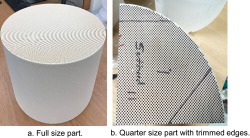
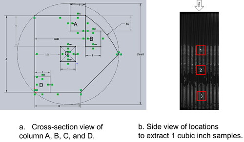
Typical PFs are cylindrical in shape and the diameter ranges from 6 inch to 12 inch, which varies with engine displacement. As a rule of thumb, a filter with a smaller diameter can be placed closer to the X-ray source with a larger magnified projection on the CT detector, resulting in a better resolution in the scan. Taking a 12 inch diameter part as an example, the image of a full-size part has the resolution of ∼ 120 µm, while a zone scan, covering a region of 1 inch diameter and 3 inch long, increases the resolution up to ∼20 µm. If the detailed ash layer profile (usually thicker than 100–300 µm) in the filter length direction is needed, an ideal image resolution should be close to 20 µm with at least 5–10 voxels in the cake thickness direction. Often, a quarter-size part provides sufficient information, where more than 2000 channels have been scanned. As shown in Figure 1b, the edges of the quarter sample are further trimmed at different angles while most of the channels are kept in the trimmed part. The functions of the trimming are two-fold. First, the part rotation diameter can be reduced by the trimming which helps to further improve the scan resolution. The rotation diameter can be reduced by 22% in the previous part preparations. Second, by trimming the two edges at different angles, it is convenient to label each channel in a cartesian coordinate system, which is quite difficult in a symmetric quarter-size part. The channel labeling turns out to be quite useful in the following data extraction and analysis.

Figure 1. Full size or trimmed quarter size DPF parts in X-ray CT scans.

2.3. Density reference preparations

Since the key information (i.e., attenuation coefficient) is typically not available from the industrial CTs, a series of density references are prepared to find the relationship between ash density and image grayscale. The aluminum capsules, as shown in Figure 2a, are used as the ash container. The raw ash deposits from the pneumatic cleaning of the real-world filters may contain certain levels of soot, which are removed via slow baking at 550 °C for two hours. After the oxidation of soot deposits, the remaining ash usually changes from black into gray color. The ICP studies show that the element compositions of baked ash are quite stable among different batches. Two representative elemental results are shown in Table 1 comparing with the counterparts from literatures. Throughout all these ICP measurements, the major metallic elements such as Ca and Zn are quite stable. The additives such as Mg and K may vary among suppliers affected by their market prices. The variance of the mean atomic number, based on the mass fraction of elements, is quite small across the listed cases. Although some literatures show quite different elemental compositions, it may arise from different lubricant formulation and measurement technique (i.e., EDS instead of ICP). So far, our experiences show that the variance of field ash mean atomic number is within 5% across the collected on-highway heavy-duty DPFs in the US. One reason could be that the lubricant oil formulation and engine operating mode are quite similar in this scenario. Meanwhile, some studies reported red and brown ash deposits from the SEM/TEM observations (Liati et al. 2012; Liati and Dimopoulos Eggenschwiler 2010). Although the main reasons accounting for the color difference is not clear, as indicated in these two papers it might be due to the high concentration of iron oxides in these collected ash samples.

Figure 2. Density reference preparation and attachment to the filter sample.

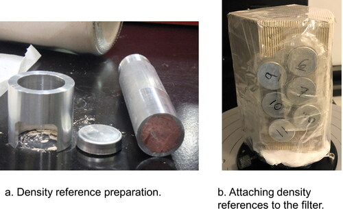
Table 1. Elemental composition of field ash via ICP.

	Weight Percentage %
Element	Ash A*	Ash B*	Ash C (McGeehan et al. 2005)	Ash D (McGeehan et al. 2009)
Ca	17.90	18.00	16.18	20.37
Zn	11.00	10.30	10.72	10.05
Mg	1.80	1.44	5.31	0.35
Fe	0.56	1.93	1.52	1.34
S	–	–	11.36	14.58
P	7.44	7.52	9.79	6.92
K	0.23	0.32	–	0.14
Na	0.20	0.91	0.23	0.88
O	–	–	43.49	41.70
Mean Atomic Number^Δ	17.50	17.99	18.65	17.92

Note: *From internal ICP measurements where elements O and S are not characterized. ^ΔDenotes that elements O and S are not counted in the mean atomic mass calculation due to lack of data in certain measurements. Some company uses more Mg in the formulation depending on the additive price.

As shown in Figure 2a, an in-house toolset is developed for the density reference preparation. The ash material is sealed inside an aluminum capsule and the diameters of the bottom holder and the upper cap are close to 1 inch to guarantee a tight seal. The rod and the cylindrical holder, shown in Figure 2a, help to align the bottom cup and the upper cap and facilitate the sealing process. Appropriate levels of compressions are applied to the filled ash to achieve the desired density. It is common that six density references are prepared with density evenly distributes between 0.2 g/cm³ and 1.0 g/cm³. The ash mass in a density reference can be calculated by the differential weight between the clean and loaded aluminum capsule. The nominal density of ash can be estimated based on the ash mass and the capsule nominal volume, which is subject to further adjustments based on the actual ash occupied volume in the capsule via CT-scan.

3. Measurement methodology

3.1. Physical principle

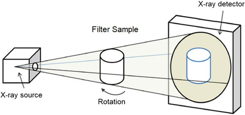
As a well-developed nondestructive characterizing method, X-ray imaging systems range from two-dimensional linear scanning (i.e., baggage check) to three-dimensional computed tomography (i.e., medical examination). The schematic drawing of the CT apparatus in current study is shown in Figure 3. The x-ray imaging techniques essentially measure the linear attenuation coefficient, µ, of the scanned sample. The absolute value of µ is rarely used in CTs. Instead, the normalized values of µ are more suitable to show the spatial distribution and local contrast for inspection and diagnostics purposes.

Figure 3. Schematic drawing of the working principle of three-dimensional CT.

The Lambert-Beer law is a fundamental physical principle that describes the x-ray attenuation along the thickness direction of a sample, as shown in Equation (1)(1) $$\frac{I}{I_0}=e^{-\mu t}$$(1) . (1) $$\frac{I}{I_0}=e^{-\mu t}$$(1)

where $I$ is the intensity of transmitted X-rays, $I_0$ is the intensity of incident X-rays, $t$ is the thickness of the sample through which X-rays have traveled. As pointed out by a previous study (Heismann, Leppert, and Stierstorfer 2003), the linear attenuation coefficient µ is related to the sample density (physical morphology) and mean atomic number (chemical classification). For X-ray energies E less than 511 keV, the photon is mainly attenuated by three mechanisms: Photoeffect absorption, Compton scattering, and Rayleigh scattering (Kelkar, Boushey, and Okos 2015). Previous studies indicate that Photoeffect absorption and Compton scattering are the dominant mechanism while Rayleigh scattering is considered as negligible (Kelkar, Boushey, and Okos 2015; Heismann, Leppert, and Stierstorfer 2003), as expressed in Equation (2)(2) $$\mu ={\mu }_{\mathit{compton}}\left(\rho ,\mathrm{ }E\right)+{\mu }_{\mathit{photo}}\left(\rho ,E,Z\right)=\left(\frac{{\mu }_{\mathit{compton}}}{\rho }\right)\rho +\left(\frac{{\mu }_{\mathit{photo}}}{\rho }\right)\rho$$(2) . (2) $$\mu ={\mu }_{\mathit{compton}}\left(\rho ,\mathrm{ }E\right)+{\mu }_{\mathit{photo}}\left(\rho ,E,Z\right)=\left(\frac{{\mu }_{\mathit{compton}}}{\rho }\right)\rho +\left(\frac{{\mu }_{\mathit{photo}}}{\rho }\right)\rho$$(2) (3) $$\left(\frac{{\mu }_{\mathit{compton}}}{\rho }\right)=\beta$$(3) (4) $$\left(\frac{{\mu }_{\mathit{photo}}}{\rho }\right)=\alpha \frac{Z^k}{E^l}$$(4)

Combining Equation (2)-(4), the relationship between density and attenuation coefficient is shown in Equation (5)(5) $$\mu =\rho \left[\beta +\alpha \frac{Z^k}{E^l}\right]$$(5) . (5) $$\mu =\rho \left[\beta +\alpha \frac{Z^k}{E^l}\right]$$(5)

where ${\mu }_{\mathit{compton}}$ is the Compton scattering attenuation coefficient and ${\mu }_{\mathit{photo}}$ is the photoeffect attenuation coefficient, ρ is the sample density, α is the photoelectric constant, $\beta$ is Compton scattering attenuation constant, Z is the mean atomic number of the scanned sample, and E is the X-ray photon energy. Typically, $\beta =0.02$ m²/kg for E < 140 keV (Heismann, Leppert, and Stierstorfer 2003), k ∼ 3 (Heismann, Leppert, and Stierstorfer 2003), and $l$ ∼ 3.1 (Cho, Tsai, and Wilson 1975). It should be noted that all the equations discussed in this section apply only to a monochromatic X-ray source.

3.2. Density-grayscale correlation in an industrial CT

The photon source in an industrial CT usually is polychromatic, instead of the monochromatic X-ray source discussed above. Thus, an equation connecting the linear attenuation coefficient and X-ray energy distribution is shown as below. (6) $$\frac{{\mu }_{\mathit{poly}}}{\rho }={\int }_{\mathit{Emi}\mathrm{n}}^{\mathit{Emax}}w\left(E\right)\left(\beta +\alpha \frac{Z^k}{E^l}\right)dE$$(6)

where ${\mu }_{\mathit{poly}}$ is the attenuation coefficient in a specific CT scan, $w(E)$ is a weighting function considering source energy spectrum and detector characteristics (Heismann, Leppert, and Stierstorfer 2003). In most of the cases, $w(E)$ is not available from CT manufacturer and may require significant effort to measure. Fortunately, $w(E)$ is same for all samples in one scan.

For a scanned PF part with attached density references, the chemical compositions of reference ash and ash deposits in a filter are same, so the right hand of Equation (6)(6) $$\frac{{\mu }_{\mathit{poly}}}{\rho }={\int }_{\mathit{Emi}\mathrm{n}}^{\mathit{Emax}}w\left(E\right)\left(\beta +\alpha \frac{Z^k}{E^l}\right)dE$$(6) for reference ash and PF ash should also be the same. Thus, Equation (7)(7) $$\left(\frac{{\mu }_{\mathit{poly},\mathrm{ }\mathit{ref}-\mathit{ash}}}{{\rho }_{\mathit{ref}-\mathit{ash}}}\right)=\left(\frac{{\mu }_{\mathit{poly},\mathrm{ }PF-\mathit{ash}}}{{\rho }_{PF-\mathit{ash}}}\right)=C_1$$(7) can be obtained as below. (7) $$\left(\frac{{\mu }_{\mathit{poly},\mathrm{ }\mathit{ref}-\mathit{ash}}}{{\rho }_{\mathit{ref}-\mathit{ash}}}\right)=\left(\frac{{\mu }_{\mathit{poly},\mathrm{ }PF-\mathit{ash}}}{{\rho }_{PF-\mathit{ash}}}\right)=C_1$$(7)

where $C_1$ is a constant and may vary with scans under different CT settings.

As known, the absolute value of ${\mu }_{\mathit{poly}}$ is not available in most industrial CT systems. However, the grayscale of ash references and ash deposits in a scanned filter, which is usually a linear transformation of the linear attenuation coefficient, is readily accessible after each scan, as shown in Equation (8)(8) $${\mu }_{\mathit{poly}}=a·gs+b$$(8) . Here gs refers to the pixel grayscale. (8) $${\mu }_{\mathit{poly}}=a·gs+b$$(8)

Since multiple density references with known ash density are scanned in the study, the relationship between ash density and CT grayscale can be obtained by combing Equations (7)-(8). (9) $${\rho }_{\mathit{ash}}=d_1·gs+d_2$$(9)

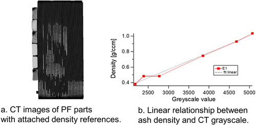
The two unknown constants in Equation (9)(9) $${\rho }_{\mathit{ash}}=d_1·gs+d_2$$(9) ,$\mathrm{ }{d}_1$ and $d_2,$ can be found through least-square fitting of the density references data, as shown in Figure 4b. The linear relationship is equally applicable to both ash density references and PF internal ash deposits. Figure 4a shows the side view of DPF #11 combined with 6 ash density references. Two of these density references use the ash removed from DPF #11 while the rest of them use ash from the pneumatic cleaning factory. Although minor levels of variances in ash elemental composition may exist, the correlation between ash density and grayscale is quasi-linear as demonstrated in Figure 4b.

Figure 4. Scan of PF part with density references and the obtained relationship between ash density and CT gray-scale.

4. Results and discussion

It is of importance to compare the CT measured density against the results from the traditional mechanical method for validation purpose. In this section, both the CT and lab mechanical approaches are used to measure ash density in small size (1 cubic inch) DPF samples. In the mechanical approach, the ash mass is obtained from the differential weight of the loaded and clean samples and the ash volume is provided by the 3 D CT scan images. It is worth noting that the mechanical measurement technique has limitations as well, where it is not physically possible to remove 100% of the ash from a filter section or absolutely eliminate the particle loss during the sample handling, and very minor amounts of the substrate may be mixed in with the ash, although these errors can be minimized by careful operations in the lab, which is described in detail in the online supplementary information.

Two quarter-size DPF parts, named DPF #11 and #12, are used in the validations. After the necessary CT scans, multiple 1 cubic inch samples, which are suitable for the mechanical density measurements, are extracted from the quarter-size parts. As shown in Figure 5a, four columns (A, B, C, and D), with a cross section of 1 inch × 1 inch and at different radial locations, are removed from the quarter-size parts with caution. Then, three segments (i.e., A1, A2, and A3) of 1 inch length are taken from each column at the designed axial locations, as illustrated in Figure 5b. From CT images, it is quite straightforward to calculate the average ash density in each cubic inch sample. In parallel, the average ash density in each cubic inch sample can be measured by the mechanical method. Although the ash volume in the small samples can be obtained by other methods (i.e., microscope imaging at the two ends of the sample), the total volume of ash in the sample is integrated by 3 D CT images, which helps to reduce the sample handling times and the resulting particle loss.

Figure 5. Taking 1 cubic inch samples from quarter-size filter for ash density validation.

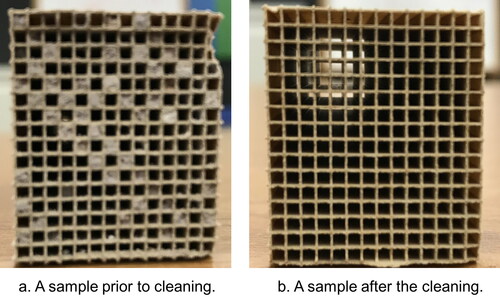
To measure the ash mass in a sample, a cleaning procedure is developed where the following steps are made: initial ambient weight, initial hot weight, pneumatic cleaning, ultrasonic cleaning, post hot weight, and post ambient weight. The samples are baked in an oven at 215 °C to remove the absorbed water and hydrated compounds and used to obtain the initial and final hot weights of measured samples. After the initial hot weight, the samples are subject to pneumatic cleaning with compressed air at a flow rate of 100 CFM. To further guarantee the cleaning effectiveness, the samples are washed in a solution with 5% citric acid for 30 min at an elevated temperature with ultrasound excitation. Figure 6 shows the samples before and after the cleaning processes. After the pneumatic and ultrasonic cleaning, the samples seem to be well cleaned and no significant deposits are found throughout the channels.

Figure 6. Comparisons of samples before and after of cleaning.

The ash density of each sample from both CT and the mechanical approach are presented in Figure 7. In total, there are 24 samples extracted from different locations of two field DPFs. The results from these two methods have quite good agreement. The average difference is approximately 8%, and the maximum difference is within 15%. This mechanical approach serves as the baseline of the comparisons, although the procedures are tedious and time-consuming. The comparisons provide a quick validation of the CT approach and increases the confidence of applying industrial CTs in the advanced analysis of PFs.

Figure 7. Comparisons of density measurements from CT and mechanical approaches.

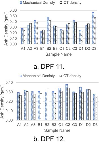
DPFs #11 and #12 are taken from on-highway heavy-duty trucks with high mileages. As indicated in Figure 7, there is no universal pattern of ash density change in DPF length and radial direction. However, in DPF #11 the ash density seems to increase in the DPF length direction except for sample B. In DPF #12 the ash density variation is rather small among the channels. In addition, it is obvious that the DPF ash density variance in DPF #11 is much larger than that in DPF #12. Figure 8 shows a detailed view of the ash profile and density distribution, where the ash distribution across channels in DPF #12 is much more uniform than that in DPF #11. In Figure 8a, the upper half of DPF #11 has ash plugs at the rear end of inlet channels while the lower half has significant intermittent mid-channel plugs. Currently, the reasons for mid-channel plug formation are not well understood. This phenomenon may be attributed to inhomogeneous and incomplete soot regeneration, extended low load operating conditions, or local hot spots causing ash sintering. From past experiences, around 10% of field DPFs show the existence of mid-channel ash plugs (Wang and Kamp 2016).

Figure 8. A detailed look of the ash density distribution in the DPF length direction.

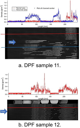
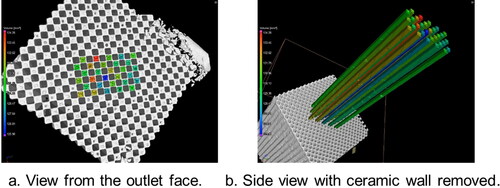
With the obtained correlation between pixel grayscale and ash density, the ash density in the three-dimensional space can be easily calculated. As shown in Figure 8, the ash density in DPF length direction is presented for DPF #11 and #12. The colored lines across DPFs indicate the channels where the ash density in the channel center is presented. Here, the void channel background (no ash existence in the center of inlet channel) shows quite low noise. This signal is not meaningful due to the absence of ash. Two channels in DPF #11 show very different density profiles. The ash density varies between 0.2 g/cm³ and 0.4 g/cm³ in most of the locations. However, inside the ash plug region, there are many bright points indicating high ash density spikes, which appear at roughly same axial location across the neighboring channels. This might be related to a strong local soot regeneration resulting in high density sintered ash.

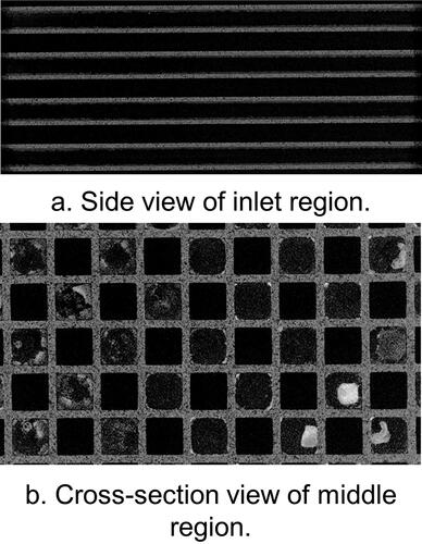
The CT image resolution is linearly related to sample rotation dimeter, since the rotation diameter dictates how close the sample can be to the X-ray source. For a quarter-size part shown in Figure 2b, a zone scan of a sub-region (1 inch diameter and 3 inch long cylinder) render a resolution of ∼12 micron. A zone scan of DPF #12 is shown in Figures 9 and 10. For the raw images from zone-scan (shown in Figure 9), even with the background noise, the ash cake layer or the partial filled channel can be seen in the inlet, middle, and outlet regions of the filter. With the assistance of image noise filter, the refined images are shown in Figure 10. As shown, even the thin ash cake layer in DPF inlet region can be clearly identified in the refined images. In addition, the bright regions in the middle region of DPF #12 in Figures 9 and 10 indicates high density or sintered ash inside the inlet channels. To process a large amount of CT images in industrial practices as shown in Figures 9 and 10, an efficient and consistent way to analyze the images is needed, which is detailed discussed in the next section for full scan images.

Figure 9. Raw images of DPF #12 zone scan.

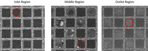
Figure 10. Refined images of DPF #12 zone scan.

5. Advanced image processing

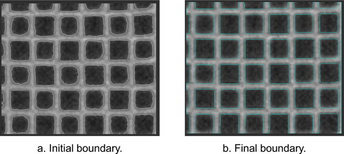
A CT image processing software, VGStudio Max V3.3, is applied to analyze the DPF ash deposit volume and density. The general procedures are listed as follow: (1) identify the boundary of ceramic wall, (2) find the regions of ash deposits and the corresponding grayscale values, (3) use density references to correlate the grayscale and ash density, and (4) export the data for additional analysis. An upper region of the DPF near the inlet face, where minor ash deposits are present, is selected to identify the ceramic wall boundary. As shown in Figure 11a, the initial substrate boundary is identified after applying a Gaussian filter, erosion filter, and a built-in surface determination. However, the detected irregular boundary is not consistent with known filter channel geometry. Thus, the dilate, erode, and shifting steps are used to refine the substrate boundary combined with region merge. An improved boundary recognition is show in Figure 11b.

Figure 11. The initial and final steps in ceramic wall boundary identification with little ash deposit.

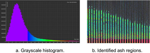
After the detection of ceramic regions, further analysis is conducted to find the ash deposit based on the histogram of the grayscale. Usually, a threshold of grayscale is found from region segmentation, where the values above are considered as ash and the rest are treated as background or ceramic walls. The optimal value comes from several iterations and the one offers the best partition between ash region and substrate wall is chosen. An example of identified ash regions based on this method is shown in Figure 12. It is worth mention that the bottom regions of Figure 12b are filter plugs that will be excluded from the analysis. Generally speaking, a scan with lower noise level is beneficial for more accurate analysis.

Figure 12. Identification of ash occupied regions based on grayscales.

Ash density references are scanned with DPF parts, which assists to find the relationship between grayscale and ash density. In preparation of the density references, the filled ash mass and capsule volume are recorded, which can be used to calculate the average ash density. The corresponding average grayscale can be obtained from the VGStudio software. As discussed in this article, the density is linearly related to X-ray attenuation coefficient or the grayscale.

As shown in Figure 13, at the end of the image processing, the digital sample is identified as three regions: ash, ceramic wall, and background (void space). Figure 13b demonstrates a three-dimensional view of the ash plugs. The power of three-dimension processing enables one to covert the grayscale data to ash density and calculate the total ash volume and mass for the regions of interested. More importantly, a well-defined protocol can be automatically applied to a batch of scanned samples, which improves the processing speed and consistency.

Figure 13. Three-dimensional view of identified ash plugs from CT images.

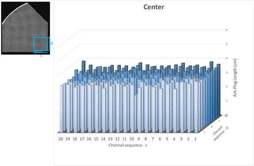
Figures 14 and 15 present the ash plug length distributions in a 12 inch diameter and 10 inch long field DPF that was harvested from a high-way heavy-duty truck with high mileage. Following the same part processing procedure, a quarter-size filter with trimmed edges was prepared for better imaging resolution and channel labeling. Figure 14 shows the periphery region ash plug distribution while Figure 15 the center region scenario, where about 200 channels were analyzed in each region. In Figure 14, it is shown that the average ash plug length is around 5 cm that generally decreases toward the center of filter (a slightly concave profile). In Figure 15, the ash plug length has a quite small variance among channels. The average ash plug length in the center region is around 3 cm, shorter than that in the periphery region. This method gives information of ash distribution from thousands of channels. With a well-developed image processing tool, it is relatively convenient and efficient to extract the ash distribution data in 3 D space.

Figure 14. Ash plug length distribution near the periphery region of field return DPF.

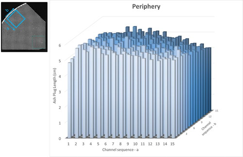
Figure 15. Ash plug length distribution near the center region of field return DPF.

6. Conclusions

In the present study, a methodology of measuring the ultra-thin PF ash deposit profile and density is developed using an industrial X-ray computed tomography (CT). With the assistances of the prepared ash references, this study confirms that the ash density is linearly related to the image grayscale. The acquired linear relationship is utilized to find the density of ash deposits in engine particulate filters.

The CT measured density values are compared with results from a dedicated laboratory method. Across 24 samples, the average difference between two methods is about 8%, which demonstrates the fidelity of the CT approach.

The means of preparing filter samples and density references in this study helps to improve the scan resolution and reduce the density measurement uncertainty. An image analysis tool is applied in processing the filter CT images, where the 3 D ash deposit analysis is accelerated with improved stability and consistency.

Considering micron-scale deposits ubiquitously exist in many processes and the density is a key property to measure, the method presented in this study may be applicable in many other fields where the traditional methods cannot meet the requirements.