Using an inkjet aerosol generator to study particle bounce in optical particle counters

Abstract

The overall counting performance of two optical particle counters (OPCs), which had a sampling flowrate of 28.3 L/min, was evaluated. An inkjet aerosol generator (IAG) was used to generate at a constant rate monodisperse test particles in the size range of 0.3–10 µm. The effect of particle phase on the counting efficiency (CE) of the two OPCs (RION KC-31 and Lighthouse Solair 1100) was characterized. Lactose monohydrate (LM) and sodium chloride (NaCl) particles were used as the solid particles. The particles of a water-soluble ionic liquid were used as the liquid particles. The CEs were evaluated for polystyrene latex (PSL) particles using a parallel comparison method. The CE of each of the two OPCs measured for solid particles was different from that measured for liquid particles. With liquid particles, the CE decreased over the micrometer range indicating that the particles had deposited on a surface within the OPC. Each CE had a sharp minimum for LM particles when the aerodynamic diameter of the particles, $d_{\mathrm{a}},$ was in the 2.5–2.6 µm range. The probability of particle bounce was evaluated using other experiments, and the results suggested that solid particles whose $d_{\mathrm{a}}$ was in the 2.6–2.9 µm range would bounce off at the inner surface of the focusing segment of the OPC, located upstream of the optical system. The CEs measured when using NaCl and PSL particles were close to unity and did not decrease over a few micrometer range; however, these particles also would bounce off.

EDITOR:

• Kihong Park

Introduction

Optical particle counters (OPCs) are used to measure the number of airborne particles in a known volume of air. The dynamic range of an OPC in terms of particle size is typically between 0.1 to a few tens of micrometers. To measure the particle number, the aerosol is drawn into the detector of the OPC through a nozzle using either an internal or external pump. Each sampled particle passes through a planarized laser beam. As the particle penetrates through the laser beam, some of the light in the beam is scattered. The amount of the scattered light first increases and then decreases. This scattered light pulse is collected by an optical lens system containing a photodiode, which converts the received light into a voltage pulse. After passing through devices that amplifies it and reduces its noise, the voltage pulse is detected and counted as a particle. An algorithm recognizes the pulse as a particle when the pulse height exceeds a threshold voltage (Borggräfe, Trampe, and Fissan 2002; Sachweh et al. 1998). Because the pulse height is related to the diameter of the sampled particle (Bohren and Huffman 1998; Kerker 1969), the pulse height is calibrated as a function of particle diameter. Polystyrene latex (PSL) particles are used as particle diameter standards in metrology. PSL particles of different sizes falling within the dynamic ranges of OPCs are commercially available, and their diameters are traceable to the metrological standard for length (ISO/TC24/SC4/WG9 2018).

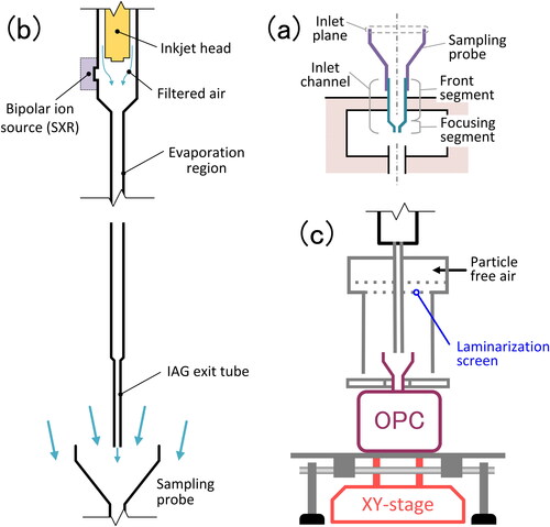
PSL particles have also been used to evaluate the counting efficiency (CE) of OPCs. Figure 1a lists the terms used in this study to describe the different parts of an OPC. The CE of an OPC depends on the counting performance of the optical sensor and the transport efficiency (TE) of the aerosol particles as they passes through the sampling probe and the inlet channel. The inlet channel consists of front and focusing segments. Figure 13 describes in detail the structure of each of these two segments. A method, which we call the parallel comparison method, was adopted in this study to evaluate the CE of an OPC when it measures PSL particles. In this method, the particle number concentration measured by the DUT-OPC1 is compared with that measured using a reference instrument, which can be a condensation particle counter (CPC) or another OPC. When a CPC is used as the reference instrument, the particle diameter range is typically below 1 µm because the TE through the flow channel of the CPC decreases as the particle size increases over the micrometer range (Sang-Nourpour and Olfert 2019; Tran et al. 2020; Yli-Ojanpera et al. 2012).

Figure 1. (a) Description of the terms used for the different parts of an OPC; sampling probe, inlet plane of the sampling probe, and the inlet channel of the OPC. The inlet channel consists of the front and focusing segments whose structure is described in detail in Figure 13. (b) Schematic of the structure of an inkjet aerosol generator (IAG), and (c) a system that can deliver IAG-generated test particles into the sampling probe of an OPC with a sampling flow rate of 28.3 L/min.

When there is a difference between the particle phase (i.e., solid or liquid) or the morphology of the PSL particles and that of the sampled particles, the measured CE can contain errors. The particle phase and particle morphology affect the collection or sampling efficiencies of inertial classification devices, such as cyclones, impactors, and virtual impactors. Particle bounce occurs when the collection substrates in these devices cannot completely absorb the kinetic energy of the colliding particles (Le and Tsai 2021). According to Cheng and Yeh (1979), a PSL particle larger than 0.8 µm in size will bounce off the surface of an uncoated collection plate when its Stokes number, $\mathit{Stk},$ is higher than 0.5. They also found that when a dioctyl phthalate (DOP) aerosol is used as the test aerosol, particle bounce does not occur. Another example is the inter-stage losses inside cascade impactors. Inter-stage losses occurred inside a Micro-Orifice Uniform Deposit Impactor (MOUDI) when the cut size was larger than 3.1 µm (Marple, Rubow, and Behm 1991). The interstage loss of oleic acid droplets was approximately 1.8 times that of solid ammonium fluorescein particles, indicating that losses due to the inertial particle motion are higher in liquid particles than in solid particles. A study on the characterization of virtual impactors for collecting bioaerosol particles showed that the wall losses of the liquid droplets of oleic acid were higher than those of PSL particles when the aerodynamic diameter, $d_{\mathrm{a}},$ of the particles exceeded 6 µm (Kesavan, Bottiger, and McFarland 2008). Chen, Yeh, and Cheng (1985) conducted an experimental study on the characterization of a virtual impactor and found that micrometer-sized liquid particles deposit easily on a surface when they decelerate because the internal circulation and deformation of the liquid in the droplets induced by aerodynamic drag reduces the drag coefficient, thereby increasing the actual stopping distance of the particles. Volckens and Peters (2005) studied the transport losses that occur inside aerodynamic particle size spectrometers and evaluated, using both solid and liquid particles, their CEs in the 0.8–10 µm particle diameter range. PSL particles 0.8, 1.0, 3.0, and 5.1 µm in diameter and ammonium fluorescein particles 9.4 µm in diameter were the solid particles used, and oleic acid particles 0.8, 1.4, 3.4, 5.7, and 10.5 µm in diameter were the liquid particles used. The CEs measured when oleic acid droplets were used, steadily decreased from 0.75 to 0.27 as $d_{\mathrm{a}}$ increased from 0.8 to 10 µm, whereas when solid particles were used the CEs measured remained steady within 0.85 and 0.99. Fluorometric analysis revealed that most of the liquid particles deposited on the tip of the inner focusing nozzle with a half angle of 60°.

The aforementioned studies suggest that particle phase could have a significant impact on the CEs of OPCs. This impact has to be considered when the airborne particle number over the micrometer range is used as a proxy for airborne microorganisms in a cleanroom. Pharmaceutical industries employ quality control protocols to evaluate the risks of cross contamination. In spacecraft assembly facilities, the microorganisms in collected particles are monitored to mitigate the biological contamination of other planets (Malli Mohan, Stricker, and Venkateswaran 2019). Microorganisms can cause cross contamination because of the endotoxins they release. Airborne microorganisms can be collected onto a culture-medium to measure their concentration in terms of colony forming unit while continuously monitoring the airborne particle number (Katayama et al. 2012; Kawai et al. 2019). Pharmaceutical guidelines (e.g., Pharmacopeia) require the monitoring of particles larger than 0.5 µm and particles larger than 5.0 µm, and the investigation of the potential risk of contamination if the particle number continuously or frequently increases beyond 5 µm. In pharmaceutical facilities, various sources, such as human skin or breath, work clothing, air conditioning equipment, and insufficiently cleaned or sterilized processes, can release microorganisms. The microorganisms in biofilms, dust piles, or liquid surfaces may get suspended in the air. The physical state of these biological particles can range from a hard crystal to a liquid of low viscosity or low surface tension.

The purpose of this study was to demonstrate that the CE of an OPC operating at a nominal sampling flowrate of 28.3 L/min over the micrometer strongly depends on the phase of the sampled particles, i.e., whether they are liquid or solid particles. To evaluate the CEs of the two ISO-compliant OPCs, an inkjet aerosol generator (IAG) (Iida and Sakurai 2018; Iida et al. 2014; Minakami et al. 2017) was used as the particle number standard. Monodisperse test particles in either solid or liquid form were generated and fed into the OPCs. In an OPC, particle bounce is an important mechanism. It enhances the TE of solid particles that are larger than a few micrometers as they move through the inlet channel of the OPC. Particle bounce has to be considered when monitoring the number of airborne particles that are proxies for biological particles.

The highlights of the sections that follow are as follows: The experimental section explains in detail how the test particles were introduced at multiple spots over the inlet plane of the isokinetic sampling probe to simulate the sampling of a uniformly mixed aerosol. It also explains another experiment which introduces test particles of different sizes as an aerosol jet onto a metal surface so that the threshold parameter of particle bounce could be determined. In the results section, how the size dependence of CE differs between solid and liquid particles is demonstrated; an argument is developed in this section to prove that particle bounce/deposition is most likely to occur at the inner surface of the focusing segment, just upstream of the optical system. The discussion section validates the argument by applying the existing semi-empirical theory on particle bounce in cascade impactors. The experimentally evaluated threshold parameter of particle bounce was used as an input to validate that the particle bounce/deposition occurred while the aerosol flow accelerated through the focusing segment of the inlet channel.

Experimental

Calibration setup

RION KC-31 (KC-31) and Lighthouse Solair 1100 (Solair 1100) are the two OPCs used in the study. Table 1 lists some of the specifications of the two OPCs. Both OPCs comply with ISO 21501-4, which describes the method of calibrating and verifying OPCs. Characterization of KC-31 produced more results than that of Solair 1100 because KC-31 was available throughout the entire period of this study. The particle size range that KC-31 and Solair 1100 could handle were 0.3–10 µm and 0.1–5.0 µm, respectively. The nominal sampling flowrate of each OPC was 28.3 L/min. The sampling probes of the OPCs were designed for isokinetic sampling within a cleanroom with a laminar flow system.¹ Figures 1b and c show the schematic description of the experimental setup used to evaluate the CEs of the two OPCs. Figure 1b illustrates the components of the IAG. The IAG contained an inkjet head, filtered air, a bipolar ion source, an evaporation tube, and an exit tube. An aqueous solution of particle material was dispensed from an inkjet head (Microdrop, MD-K-130) at a fixed rate. The nozzle diameter of the inkjet head was 30 µm. The droplet generation rate, $f_{\mathrm{d}}$ (s⁻¹), of the inkjet head was fixed at 30.00 s⁻¹ throughout the study. A photoionizer (L11757, Hamamatsu) was used as the bipolar ion source. The ions produced by the photoionizer electrically neutralized the dispensed droplets. The droplets were transported through an evaporation tube whose wall was heated at 80, 100, or 110 °C. The inner diameter and length of the tube were 10.2 mm and 410 mm, respectively. The flowrate through the tube was maintained at 0.15 L/min, and the approximate average of the transport time through the tube was 13 s. When the solvent in the droplets evaporated, the solute became an aerosol particle. The particles exited through the exit tube of the IAG whose effective inner diameter² was 2.47 mm at its tip, the corresponding aerosol flow velocity was 0.53 m/s. The average aerosol velocity at the inlet plane of KC-31 and Solair 1100 were 0.45 m/s and 0.51 m/s, respectively. The aerosol velocity at the tip of the IAG exit tube (0.53 m/s) did not significantly exceed the average aerosol velocity over the inlet planes of the two OPCs (0.45 m/s or 0.51 m/s); therefore, the aerosol jet from the IAG exit tube did not generate any strong turbulence over the inlet plane of the sampling probe.

Table 1. Specifications of the OPCs used in the study.

Manufacturer and model	Unit	RION, KC-31	Lighthouse, Solair 1100
Nominal sampling flowrate	L/min	28.3	28.3
Size settings	µm	0.3, 0.5, 1.0, 2.0, 5.0, 10	0.1, 0.2, 0.3, 0.5, 1.0, 5.0
Inner diameter of sampling probe	mm	36.5	34.4
Optical configuration		λ = 780 nm α = 70°	Not disclosed

Figure 1c shows the system used to deliver the test particles generated by the IAG to the DUT-OPCs. Each OPC was placed on a platform which moved horizontally to bring the tip of the IAG exit tube to a specific spot over the inlet plane of the sampling probe. The platform was attached to a motorized XY-stage (Model OSMS26-100(XY), Sigma-Koki, Japan). The stage was operated using a controller and its associated software (Model SHOT-202 and SG Commander, Sigma-Koki, Japan). Because the aerosol flowrate in the IAG was only 5.3% of the sampling flowrate of the OPC, particle-free air was supplied as a sheath flow to the flow chamber through a laminarization screen as shown in Figure 1c. The inner diameter of the chamber was 114 mm. The flowrate of the supplied particle-free air, $Q_{\mathrm{cham}},$ was set at 45 L/min. The distance from the laminarization screen to the inlet plane of the sampling probe was 130 mm. At high values of $Q_{\mathrm{cham}},$ turbulence occurred near the inlet plane of the sampling probe. Figure 2 shows the effect of $Q_{\mathrm{cham}}$ on the pulse height distribution measured by KC-31.

Figure 2. Effect of the flow rate in the sheath flow chamber on the pulse height distributions measured by an OPC (RION KC-31). The test particles are made of lactose monohydrate with $d_{\mathrm{v}}$= 8.2 µm. The particles are introduced along the center axis of the sampling probe.

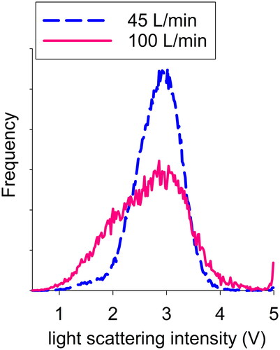
The IAG was used to generate lactose monohydrate (LM) particles with a volume equivalent diameter of 8.2 µm. The particles were introduced along the center axis of the sampling probe. The monodispersity of pulse height distribution decreased when $Q_{\mathrm{cham}}$ was increased from 45 to 100 L/min. The increased width of the distribution indicated that the turbulence that occurred at high values of $Q_{\mathrm{cham}}$ dispersed the test particles in space. This type of dispersion is undesirable because it reduces the accuracy of the position from where the particles are delivered to the inlet plane of the sampling probe. At $Q_{\mathrm{cham}}$= 45 L/min, the average particle velocity in the chamber was 0.073 m/s, which was 6.1–6.9 times smaller than the particle velocity at the inlet plane of the sampling probe; therefore, the OPC was sampling under a super-isokinetic condition. Equation (1)(1) $$R\mathrm{e}=\frac{4{\rho }_{\mathrm{a}}{Q}_{\text{cham }}}{\pi \mu W_{\mathrm{cham}}}$$(1) given below was used to calculate the Reynolds number, $Re.$ (1) $$R\mathrm{e}=\frac{4{\rho }_{\mathrm{a}}{Q}_{\text{cham }}}{\pi \mu W_{\mathrm{cham}}}$$(1) where$Q_{\mathrm{cham} }$ (m³/s) is the flowrate of the particle free air, ${\rho }_a$ (kg/m³) is the density of air, $\mu$ (Pa⋅s) is the dynamic viscosity of air, and $W_{\mathrm{cham}}$ (m) is the diameter of the chamber. The $Re$ inside the chamber was 530 indicating a laminar flow regime.

Figure 3 shows examples of the particle delivery patterns over the inlet plane of the sampling probes of the two OPCs. When evaluating the CE of KC-31, the patterns shown at the top (Figures 3a and b) were used. The particles were delivered to a set of fixed points. The dashed lines divide the inlet plane to four segments which have an equal-flowrate. As shown in Figure 3a, the areas of the segments become equal if a plug flow or an inviscid flow is assumed. When a parabolic flow or viscous flow is assumed, the areas of the equal-flow segments increase as the radial position,$r,$ increases. Because the functional form of parabolic flow is $1-{(r/R)}^2,$ which non-linearly decreases to zero as $r$ increases, the larger areas have to be integrated to let the same volume of air pass through them. The same number of particles were delivered to each segment to simulate particle flux (particles m⁻² s⁻¹) for a plug or parabolic flow.³ KC-31 and the XY-stage were operated remotely by sending commands and receiving data in a programmed loop. The sampling time of KC-31 was set to 551 s, which was the approximate time required to travel through the 32 points shown in Figures 3a and b.⁴ To evaluate the CE of Solair 1100, the pattern shown at the bottom of Figure 3 (Figures 3c and d) was used. The particles were delivered to a set of randomly generated points. The online supplementary information (SI) presented explains the method used to generate these delivery points. 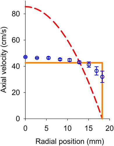A condition under which the cumulative distribution of the particle delivery points matched well with that of the flowrate when plotted as a function of $r,$ was searched for. To evaluate the CE of Solair 1100, the sampling time of the OPC was set at 660 s. The number of particles delivered to the OPC was 19,800. The operation of the XY-stage was independent of the OPC, and the test particles were delivered to randomly generated points. To simulate the sampling of aerosol particles inside a cleanroom, the velocity distribution of the particles over the inlet plane of the sampling probe had to be known (Iida and Sakurai 2018). A hot-wire anemometer (Model 6034, Kanomax, Japan) was used to measure the velocity distribution of the particles as a function of their radial positions.⁵ A spherical probe with a diameter of 2.5 mm (Model 6543-21, Kanomax, Japan) was used. As shown in Figure 4, the measured axial velocity distribution of the particles was bounded by plug and parabolic flows.

Figure 3. Illustration of the particle delivery patterns over the inlet plane of the sampling probe. When the CE of KC-31 was evaluated, the patterns shown on the upper side (a and b) were used; the particles were delivered to a set of fixed points. When the CE of Solair 1100 was evaluated, the pattern shown on the lower side (c and d) were used; the particles were delivered to a set of randomly generated points. The patterns shown on the left side (a and c) and right side (b and d) assume that the velocity profile of the incoming aerosol relates to plug flow and parabolic flow, respectively. The method of preparing the delivery patterns with randomly generated points is explained in the supplementary material provided.

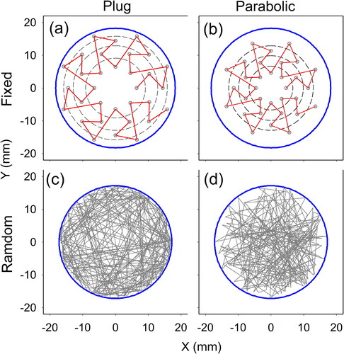
Figure 4. Distribution of the axial velocity over the inlet plane of the sampling probe of KC-31 as a function of the radial position. The circles with error bars indicate measured values. Solid and dashed lines denote the velocity distribution in plug and parabolic flows, respectively.

Test particles

Table 2 lists the test particles generated by the IAG to enable the evaluation of the CEs of the two OPCs. The concentration of the solute in each inkjet solution, $C_{\mathrm{m}},$ and the volume equivalent diameter of the particles generated by the IAG, $d_{\mathrm{v}},$ also are listed. $d_{\mathrm{v}}$ ranges from 0.3 µm to 10 µm approximately. The method used to calculate $d_{\mathrm{v}}$ is described in the SI. Three types of particle materials were used: LM (128-00095, WAKO Pure Chemical, Japan), 1-ethyl-3-methylimidazolium trifluoromethanesulfonate (TFMS; 059-07111, Wako Pure Chemical, Japan), and sodium chloride (NaCl; 198-01675, Wako Pure Chemical, Japan). LM is a water-soluble organic solid. Its material density was measured using the volumetric displacement method (ISO/TC24/SC4/WG3 2014). Microscopic observations showed that LM particles were nearly spherical (Minakami et al. 2017). TFMS is a water-soluble ionic liquid. Its material density was measured using an oscillation-type density meter (DMA 5000 M, Anton Parr). The NaCl particles generated by the IAG were agglomerates of cubic crystals (Iida et al. 2014). Their material density was taken from a database (CRC 2013). A demo KC-31 unit was used when the CEs of the OPCs were measured when using LM and TFMS particles. A commercial KC-31 was used when the CE was measured using NaCl particles.⁶ The structure and design of the two units were identical.

Table 2. List of test particles generated by the IAG, their concentrations in the inkjet solution, $C_{\mathrm{m}};$ volume equivalent diameter, $d_{\mathrm{v}};$ optical diameter, $d_{\mathrm{o}};$ and aerodynamic diameter, $d_{\mathrm{a}},$ of the test particles.

Name of solute	Lactose monohydrate (LM)				1-Ethyl-3-methylimidazolium trifluoromethanesulfonate (TFMS)				Sodium chloride (NaCl)
Mass density	1.540 g/cm^3				1.380 g/ml				2.17 g/cm^3
Parameter	$C_{\mathrm{m}}$^a	Particle diameter, µm			$C_{\mathrm{m}}$^a	Particle diameter, µm			$C_{\mathrm{m}}$^a	Particle diameter, µm
		$d_{\mathrm{v}}$	$d_{\mathrm{o}}$	$d_{\mathrm{a}}$		$d_{\mathrm{v}}$	$d_{\mathrm{o}}$	$d_{\mathrm{a}}$		$d_{\mathrm{v}}$	$d_{\mathrm{o}}$	$d_{\mathrm{a}}$
KC-31	0.0688 0.2051 1.516 7.301 13.36 13.36 71.01 199.3 275 1665 1668 7391 13260 13260	0.243, i 0.291, i 0.498, i 0.824, i 0.910, ii 1.01, i 1.59, ii 2.24, ii 2.49, ii 4.54, ii 5.01, i 8.23, i 9.06, ii 10.0, i	0.292 0.410 0.523 0.726 1.06 1.06 1.93 2.56 2.72 4.49 4.86 8.56 10.2 9.95	0.696 1.11 1.20 1.31 1.98 2.56 2.71 5.58 6.23 10.3 11.8 11.6	0.2263 0.3303 0.5054 1.272 6.709 12.97 63.88 269.9 1503 6508 11390	0.305, i 0.333, i 0.373, i 0.488, i 0.831, i 1.03, i 1.59, ii 2.57, ii 5.02, i 8.18, i 9.86, i	0.275 0.301 0.335 0.422 0.788 1.15 1.98 2.67 5.14 8.55 9.81	– – − 0.648 0.977 1.23 1.94 2.87 5.91 9.73 11.2	0.6375 2.015 6.375 20.15 63.6 201.8 633.5 1094 2012 3595 6292 19770	0.353, iii 0.493, iii 0.710, iii 1.04, iii 1.52, iii 2.23, iii 3.26, iii 3.91, iii 4.79, iii 5.82, iii 7.01, iii 10.3, iii	0.424 0.451 0.687 1.05 2.31 2.68 4.06 5.25 6.36 7.46 9.04 12.0	– 0.678 0.889 1.32 1.98 2.64 3.70 4.62 5.95 7.37 8.85 12.6
Solair 1100	0.2038 0.6767 0.9684 2.030 9.653 20.29 96.46 349.4 706.2 2236 2641 3473 7933 12860 17750	0.250, iv 0.361, iv 0.404, iv 0.515, iv 0.861, iv 1.10, iv 1.85, iv 2.85, iv 3.60, iv 5.29, iv 5.59, iv 6.13, iv 8.07, iv 9.48, iv 10.6, iv	0.209 0.402 0.418 0.397 0.719 0.901 2.25 2.65 3.34 5.35 5.73 6.50 9.13 10.9 12.1	0.719 1.15 1.42 2.24 3.40 4.34 6.62 7.04 7.77 10.2 11.6 12.6	1.984 19.82 197.9 1964 8498 15970	0.530, iv 1.14, iv 2.45, iv 5.26, iv 8.57, iv 10.6, iv	0.253 0.791 2.53 5.19 8.76 11.3	0.683 1.37 2.77 6.26 10.1 11.7

^a $C_{\mathrm{m}}$ has no units because it is equal to (mass of solute/mass of solution)$\times {10}^{-6}.$

i Average mass of a droplet $m_{\mathrm{d}}$ = 60.84 $\times {10}^{-12}$ kg and the diameter of the solvent residue $d_{\mathrm{r}}$ = 210 ± 33 nm.

ii $m_{\mathrm{d}}$ = 45.20 $\times {10}^{-12}$ kg and $d_{\mathrm{r}}$ = 153 ± 29 nm.

iii $m_{\mathrm{d}}$ = 62.16 $\times {10}^{-12}$ kg and $d_{\mathrm{r}}$ = 155 ± 38 nm.

iv $m_d$ = 53.14 $\times {10}^{-12}$ kg and $d_{\mathrm{r}}$ = 128 ± 27 nm.

As the results section shows, the CEs measured when LM and NaCl particles were used were remarkably different from those measured when TFMS particles were used. To investigate the dependence of the CE on the type of particle material used, PSL particles were used as test particles. The CEs were evaluated by making a parallel comparison of the particle number concentrations measured using a DUT-OPC and a reference instrument (ISO/TC24/SC4/WG9 2018). The experiment was performed at the OPC calibration facility of the Federal Institute of Metrology METAS (Wabern, Switzerland), a custom-made experimental facility, which consists of an aerosol generation system, a turbulent flow tube (homogenizer), and a particle detection system (Horender, Auderset, and Vasilatou 2019; Vasilatou et al. 2020). The diameters of the PSL particles used were 1.005, 2.742, and 5.067 µm.

Optical and aerodynamic diameters of the test particles

The optical diameters of the particles generated by the IAG were evaluated by analyzing the pulse-height distribution of the signals produced by the scattered light. The procedure given in ISO 21501-4 was used as a guideline in calculating the representative pulse-height voltage of the measured distribution (ISO/TC24/SC4/WG9 2018). The PSL-equivalent optical diameter,${ d}_{\mathrm{o}},$ corresponding to the measured pulse height voltage was evaluated using spline interpolation of the size-calibration curve.⁷ The aerodynamic diameter,$d_{\mathrm{a}},$ was measured using an Aerodynamic Particle Sizer (APS, Model 3321, TSI Inc.). The particle size measured by the APS was calibrated by its manufacturer. The software used in the APS (Aerosol Instrument Manager, AIM) produced an aerodynamic size distribution. $d_{\mathrm{a}}$ refers to the number-based average diameter of the measured size distribution. In our previous study $d_{\mathrm{a}}$ for NaCl/TFMS particles was expressed as a function of $d_{\mathrm{v}}$ (Iida et al. 2014). The value of $d_{\mathrm{a}}$ corresponding to the value of $d_{\mathrm{v}}$ was evaluated through the spline interpolation of our previous data. The $d_{\mathrm{a}}$ for LM particles was measured. $d_{\mathrm{o}}$ and $d_{\mathrm{a}}$ of the test particles generated by the IAG are listed in Table 2.

KC-31 performed pulse height analysis (PHA) internally. Using a USB cable, KC-31 was connected to a notebook computer that had PHA software (KL-50A, RION) installed. Solair 1100 had an analog output port and the output signal was proportional to the intensity of the scattered light on a logarithmic scale. The intensity of the scattered light was calibrated as a function of the PSL particle diameter. Table 3 lists the type of PSL particles (JSR Life Science, Japan) used and the method used for aerosolizing them. The table also includes the protocol used for preparing the diluted PSL suspensions that were aerosolized. PSL particles less than or equal to 0.814 µm in size were aerosolized using an atomizer (Aeromaster V, JSR Corporation, Japan), which had a dilutor and a dryer. The dried aerosol was electrically neutralized and classified using a differential electrical mobility classifier (DEMC; Model 3081, TSI Inc.), which selected the PSL particles and removed the residue particles. PSL particles with sizes larger than or equal to 0.814 µm were aerosolized using an IAG. The particles were suspended in isopropyl alcohol. $f_{\mathrm{d}}$ was set to 120 s⁻¹ during the dispensing of the suspension.⁸ The inkjet process consumed only 60–70 µl of the PSL suspension during an hour of operation when the size of the inkjet nozzle was 70 µm. Thus, as Table 3 shows, less than 0.1 ml of the PSL suspension was required when an IAG was used to aerosolize the PSL particles.

Table 3. List of PSL particles^a and aerosolization methods.

Method for aerosolization	Average diameter in the certificate	Volume of PSL taken from the product bottle, µl	Volume of dispersion medium, ml
Atomization of aqueous suspension^b of PSL particles followed by electrical neutralization and mobility classification. Dispersion medium: ultrapure water	0.254 µm	110	100
	0.309 µm	170	100
	0.352 µm	300	100
	0.402 µm	300	100
	0.506 µm	300	100
	0.603 µm	300	100
	0.814 µm	700	100
Inkjet aerosol generator^c Dispersion medium: isopropyl alcohol	0.814 µm	2	100
	1.005 µm	2	100
	2.005 µm	28	100
	3.21 µm	31	100
	5.124 µm	22	20
	7.088 µm	31	10
	10.04 µm	85	10

^a PSL products with particle diameters below 3 µm are called STADEX, the products with other particle sizes are called DYNOSPHERES. The solid content of the products is 1%. The products have been discontinued in April 2019.

^b Aeromaster V atomizer (JSR Corporation, Japan), which now is obsolete, was used as the atomizer.

^c The nozzle diameter of the inkjet head was 70 µm. $m_{\mathrm{d}}$ = 186 × 10⁻¹²kg was assumed based on the measurements done with water as the inkjet solution.

A size calibration table was stored in the internal memory of Solair 1100. Particle diameters 0.1, 0.15, 0.2, 0.25, 0.3, 0.5, 1.0, and 5.0 µm were listed in the table. Because the number of particle sizes in the micrometer range was only a few, to evaluate the optical diameters of the test particles, new sizes were included in the table. The IAG aerosolized the PSL particles, which were 2.005, 3.21, 5.124, 7.088, and 10.04 µm in diameter. New calibration data pertaining to these sizes were generated. These new data were combined with the stored data for the diameters 0.1, 0.15, 0.2, 0.25, 0.3, 0.5, and 1.0 µm. The analog signals were sent to a high-speed digitizer (PXIe-5122, NI, USA), whose input and output were controlled and processed using a PC and a LabView-based PHA program.

Evaluation of the CEs of the OPCs and their uncertainties

When an IAG is used as a particle number concentration standard, the CE of an OPC is defined as the ratio of the particle count rate of the OPC, $L,$ to the particle generation rate of the IAG, $L_{\mathit{IAG}}.$ The particle count rate of the OPC is evaluated by the number of particles detected by it,$N,$ divided by the OPC sampling time, $t.$ (2) $$L=\frac{N}{t}$$(2)

$L$ was measured five times for a given particle delivery pattern in which the particle velocity profile over the inlet plane of the sampling probe was assumed to be either plug or parabolic in shape. ${\overline{L}}_{\mathrm{plug}}$ and ${\overline{L}}_{\mathrm{parablic}}$ are the average values obtained by the five repeated measurements. Because the true particle velocity profile was unknown, the probability density function $\mathrm{\psi }\left(L\right)$ was applied to the particle count rate. Figure 5 shows the function $\mathrm{\psi }\left(L\right).$

Figure 5. Probability density function of the particle count rate, $L.$ Asymmetric triangular distribution gives weight to ${\overline{L}}_{\mathrm{plug}},$ the particle count rate which assumes that the flow profile over the inlet plane is plug flow.

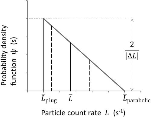
The function $\mathrm{\psi }\left(L\right)$ is an asymmetric triangular distribution with its maximum at ${\overline{L}}_{\mathrm{plug}}.$ It linearly decreases to zero at ${\overline{L}}_{\mathrm{parablic}}.$ The function considers that the flow profile over the inlet plane is more like a plug flow than a parabolic flow as it is shown in Figure 5. (3a) $$\mathrm{\psi }\left(L\right)=\frac{2}{\left|\mathrm{\Delta }\overline{L}\right|\mathrm{\Delta }\overline{L}}\left({\overline{L}}_{\mathrm{parablic}}-L\right)$$(3a) (3b) $$\mathrm{\Delta }\overline{L}={\overline{L}}_{\mathrm{parablic}}-{\overline{L}}_{\mathrm{plug}}$$(3b)

The representative value $\overline{L}$ of $\mathrm{\psi }\left(L\right)$ is given by (4a) $$\overline{L}=\frac{1}{3}(2{\overline{L}}_{\mathrm{parablic}}-{\overline{L}}_{\mathrm{plug}})$$(4a)

Then CE is calculated as (4b) $$CE=\frac{\overline{L}}{L_{\mathrm{IAG}}}$$(4b)

The uncertainty of CE is evaluated using error propagation. (5a) $${\left(\frac{u\left(CE\right)}{CE}\right)}^2\cong {\left(\frac{u\left(L_{\mathrm{IAG}}\right)}{L_{\mathrm{IAG}}}\right)}^2+{\left(\frac{u\left(\overline{L}\right)}{\overline{L}}\right)}^2$$(5a) $\mathrm{u}\left(L_{\mathrm{IAG}}\right)/L_{\mathrm{IAG}}$ the relative standard uncertainty (RSU) of the particle generation rate. The value of $L_{\mathit{IAG}}$ is given by (5b) $$L_{\mathrm{IAG}}={\eta }_{\mathrm{IAG}}·F$$(5b) where $F$ is the frequency of the voltage pulses sent to the piezoelectric element of the inkjet head. The symbol ${\eta }_{\mathrm{IAG}}$ refers to the particle generation efficiency of the IAG, which is the efficiency of generating a particle from a voltage pulse sent to the inkjet head. ${\eta }_{\mathrm{IAG}}$ was evaluated using separate experiments. Its average value was 0.9995, indicating that the particle loss inside the IAG was negligible. Thus, ${\eta }_{\mathrm{IAG}}$ was assumed to be unity. The systematic error caused by this assumption was included in the uncertainty of ${\eta }_{\mathrm{IAG}}.$ In summary, the RSU of $L_{\mathrm{IAG}}$ was 0.0026 when $L_{\mathrm{IAG}}$ was between 10 and 100 s⁻¹. The$u\left(\overline{L}\right)/\overline{L}$ is the RSU of $\overline{L}.$ It has random and systematic components. (5c) $${\left(\frac{u\left(\overline{L}\right)}{\overline{L}}\right)}^2\cong {\left(\frac{u_{\mathrm{rand}}\left(\overline{L}\right)}{\overline{L}}\right)}^2+{\left(\frac{u_{\mathrm{sys}}\left(\overline{L}\right)}{\overline{L}}\right)}^2$$(5c)

The random component is the measurement repeatability. Its value was evaluated by analysis of variance (ANOVA). The input matrix of the ANOVA consisted of 2 × 5 values of $L$ where 2 and 5 correspond to the number of flow profiles and repeated measurements, respectively. The systematic component was estimated using the standard width of $\mathrm{\psi }\left(L\right),$ and it considers that the true particle flux is unknown. (5d) $$u_{\mathrm{sys}}\left(\overline{L}\right)=\frac{1}{3\sqrt{2}}\left|\mathrm{\Delta }\overline{L}\right|$$(5d)

Direct evaluation of particle bounce

As indicated in the results section, the CEs of the two OPCs were strongly influenced by the particle phase (i.e. whether they were solids or liquids). Additional experiments were performed using KC-31 to confirm that the solid particles bounce off the OPC surface and that liquid particles deposit on it. Figure 6 illustrates the experimental setup used.

Figure 6. Illustration of the experiments conducted to confirm that the solid particles bounce off a surface while liquid particles deposit on it. An approximate gap of 1 mm existed between the tip of the IAG exit tube (inner diameter: 1.2 mm) and the surface of the stainless-steel ball (6.35 mm in diameter). The inner diameter of the sampling probe was 36.5 mm. The average velocity of the aerosol flow at the exit of the tube was 2.2 m/s.

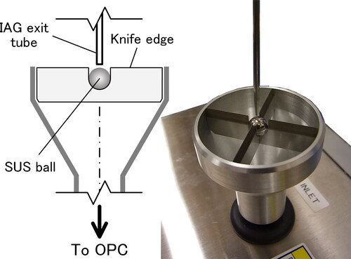
The setup simulates a stagnation flow within an axisymmetric system. In the experiment, an IAG exit tube with an inner diameter of 1.15 mm was used. The velocity of the aerosol flow was 2.4 m/s. A stainless-steel ball, 6.4 mm in diameter, was placed 1 mm below the tip of the tube. KC-31 detected the particles that bounced off the surface without depositing on it. Three types of particle materials were used: LM, TFMS, and NaCl. $d_{\mathrm{v}}$ was varied from 0.5 µm to 12 µm approximately.

Results

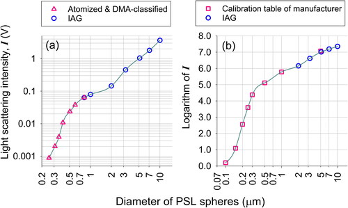
Figure 7 shows the intensity of the scattered light as a function of PSL particle diameter. These calibration curves were used to evaluate the $d_{\mathrm{o}}$ of the particles generated by the IAG. The results demonstrated that the IAG can efficiently aerosolize PSL particles up to 10 µm in size.

Figure 7. Intensity of the scattered light as a function of the PSL particle diameter plotted for (a) KC-31 and (b) Solair 1100. (▵) Aqueous suspensions of PSL particles were aerosolized using an atomizer and classified subsequently using a differential mobility analyzer, (◯) PSL particles were suspended in isopropyl alcohol, and the suspension was used as the inkjet solution of the IAG. (□) Calibration data stored in the internal hardware of Solair 1100. The lines are spline curves. Spline interpolation was used to find the value of $d_{\mathrm{o}}$ for a given intensity of IAG-generated particles, and the interpolation was performed on a log-log scale.

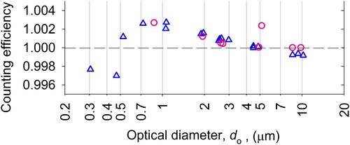
Figure 8 shows the CE of KC-31 when the tip of the IAG exit tube was aligned with the center axis of the sampling probe. The CE values were within 1.000 ± 0.005, indicating that all the particles generated by the IAG were delivered to the optical sensor of the OPC and counted irrespective of whether they were solid or liquid particles.

Figure 8. Counting efficiency of KC-31 as a function of optical diameter. The center axis of the IAG exit tube was aligned with the center axis of the sampling probe. LM is a solid. TFMS is a water-soluble ionic liquid.

Figures 9a and b show the CE of KC-31 as a function of the optical diameter in the 0.3–10 µm range and aerodynamic diameters larger than 1 µm, respectively. An equal number of particles were delivered to 32 spots over the inlet plane of the sampling probe as shown in Figures 3a and b to simulate aerosol sampling within a cleanroom environment. The optical diameter is chosen here to describe the size-dependent trend shown in Figure 9.

Figure 9. Counting efficiency of KC-31 as a function of (a) optical and (b) aerodynamic diameters. Test particles were introduced uniformly over the inlet plane of the sampling probe to simulate the sampling of airborne particles in a clean room environment. LM and NaCl are solids, and TFMS is a liquid.

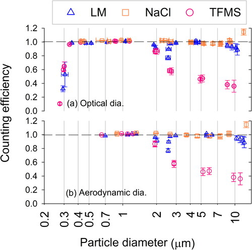
Remarkable differences exist between the measured CE for solid and liquid particles larger than 2 µm in size. The measured CE for TFMS particles steadily decreased with increasing particle size. As the particle size increased from 2.0 to 9.8 µm, the measured CE decreased non-linearly from 0.88 to 0.39. The measured CE for LM particles over the micrometer range reached a sharp minimum when the particle size was approximately 2.5 µm. It increased from 0.78 to 0.99 as the particle size increased from 2.5 to 3.0 µm. It was 1.0 again at 5 µm and remained at that value up to an approximate particle size of 7 µm. It decreased again from 0.96 to 0.91 as the LM particle size increased from 8.6 to 10.5 µm. There are two differences in the CEs measured with NaCl and LM particles. First, the CE measured for NaCl particles does not show any significant decrease in the particle size from 2 to 3 µm. It remains constant between the particle sizes of 0.4 and 7.5 µm. Second, it increased from 1.01 to 1.2 as the particle size increased from 7.5 to 12 µm.

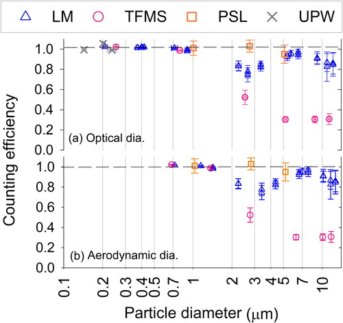
Figure 10 shows the measured CE of Solair 1100 as a function of the (a) optical and (b) aerodynamic diameters. The size-dependent trend of Solair 1100 qualitatively is same as that of KC-31, which can be explained using the optical diameter. The measured CE when liquid TFMS particles were used decreased from 1.02 to 0.30 as the particle size increased from 0.8 to 11.3 µm, and was 0.52 at a particle size of 2.6 µm. With LM particles, it had a sharp minimum at an approximate particle size of 2.6 µm. The measured CE increased from 0.76 to 0.95 as the particle size increased from 2.6 to 5.9 µm. It decreased again from 0.95 to 0.85 as the particle size increased from 8.6 to 11.5 µm. The measured CEs for PSL particles 1.0, 2.7, and 5.1 µm in size were close to unity. They were evaluated at METAS using the parallel comparison method.

Figure 10. Counting efficiency of Solair 1100 as a function of (a) optical and (b) aerodynamic diameters. Test particles were introduced uniformly over the inlet plane of the sampling probe. LM and TFMS have solid and liquid particles, respectively. Ultrapure water (UPW) was used as the inkjet solution of the IAG. The particles are evaporation residues of ultrapure water. The CEs for the PSL particles were evaluated using the parallel comparison method. The aerodynamic diameters of the PSL particles were calculated from the certified diameters and the assumed mass density (= 1.05 g/cm³) provided by the manufacturer. The typical temperature (= 30 °C) and pressure (= 1010 hPa) inside the aerodynamic particle sizer were used in the calculations.

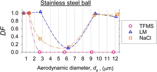
Figure 11 shows the results of the experiment in which a stainless-steel ball was placed below the tip of the IAG exit tube to induce an inertial impaction of the solid and liquid particles generated by the IAG. The results can be expressed by plotting the detected fraction (DF) against the aerodynamic diameter because KC-31, which was located downstream of the ball, detected the particles that did not deposit on the surface. As the figure shows, none of the liquid particles (TFMS) equal to or greater than 3 µm in size were detected by the OPC. The DFs of the solid particles (LM and NaCl) attained their minimum values, which were in the 0.10–0.14 range, when $d_{\mathrm{a}}$ was in the 6.2–6.4 µm range. The DF of the solid particles increased and exceeded 0.95 for particle sizes larger than 9.2 µm.

Figure 11. The fraction of the detected particles (DF) as a function of the aerodynamic diameter when a stainless-steel ball was placed approximately 1 mm below the tip of the IAG exit tube (Figure 6). Lines were added to lead the eyes to each particle type. The smallest size at which the particle bounce occurs is greater than 6.2 µm but less than 9.4 µm.

Discussion

The solid particles bounced off from the OPC surfaces, whereas the liquid particles deposited on the surfaces. A difference existed between the CEs measured with solid particles and those measured with liquid particles for particle sizes larger than 2 µm approximately. Because the aerosol flow velocity was highest in the inlet channel, the particle deposition/bounce was assumed to occur while the aerosol flow accelerated through the inlet channel (Figure 1a). This section uses the model used for particle bounce in cascade impactors to validate the assumption. The last part of the section discusses the CE measured with solid particles that were larger than 7 µm approximately.

General relationship of particle bounce

The general mathematical relationship of particle bounce was applied to the experimentally observed trend to enable the direct evaluation of particle bounce. An equation for the probability of particle bounce for LM and NaCl particles was developed thereafter. Particle bounce has been studied in the past when evaluating its effect on the collection efficiency of cascade impactors. The Stokes number, $\mathit{Stk},$ at the exit of a round nozzle of an impactor is given by Marple and Olson (2011) (6) $$\mathit{Stk}=\frac{4\rho Q{C}_{\mathrm{c}}{d}_{\mathrm{s}}^2}{9\pi \mu W^3}$$(6) where $\rho$ (kg/m³) is the density of the particle,$Q$ (m³/s) is the flowrate through the round nozzle, $C_{\mathrm{c}}$ is the slip correction factor, $d_s$ (m) is the Stokes diameter, and $W$ (m) is the nozzle diameter of the impactor. The aerodynamic behavior of the test particles with different particle densities were compared on the same basis. Because the definition of the measured particle size is the aerodynamic diameter, $d_{\mathrm{a}}$ the value of $\rho$ in Equations (6)(6) $$\mathit{Stk}=\frac{4\rho Q{C}_{\mathrm{c}}{d}_{\mathrm{s}}^2}{9\pi \mu W^3}$$(6) and (7b)(7b) $$\mathrm{\gamma }=U_{\mathrm{i}}{d}_{\mathrm{s}}\sqrt{\frac{\rho }{{\rho }_0}}$$(7b) below was taken as unity (${\rho }_0=$ 1 g/cm³ or 1000 kg/m³); $d_{\mathrm{s}},$ therefore, was equal to $d_{\mathrm{a}}.$ The value of $\mathit{Stk}$ at which the collection efficiency is 50% is called${\mathit{Stk}}_{50},$ and for an impactor with a round nozzle $\sqrt{{\mathit{Stk}}_{50}}=$0.47. For example, if $W$ in Equation (6)(6) $$\mathit{Stk}=\frac{4\rho Q{C}_{\mathrm{c}}{d}_{\mathrm{s}}^2}{9\pi \mu W^3}$$(6) is set to the effective inner diameter of the IAG exit tube [2.47 mm, Figure 1b], and if $Q$ in Equation (6)(6) $$\mathit{Stk}=\frac{4\rho Q{C}_{\mathrm{c}}{d}_{\mathrm{s}}^2}{9\pi \mu W^3}$$(6) is set to the aerosol flowrate of the IAG (0.15 L/min), $\sqrt{Stk}$ for $d_{\mathrm{a}}$= 10 µm at the exit tube of the IAG is 0.25. Because the obtained value of $\sqrt{Stk}$ is smaller than 0.47, the aerosol jet at the IAG exit tube would not induce inertial impaction of the test particles at the edge of the sampling probe. Cheng and Yeh (1979) presented a general relationship that can be used to determine the probability of particle bounce of LM and NaCl particles. The velocity of a particle, $U_{\mathrm{i}},$ when the particle impacts on a substrate can be estimated as follows for values of$\mathit{Stk}$ larger than${\mathit{Stk}}_{50}$ (7a) $$\frac{U_{\mathrm{i}}}{U}=1-\frac{1}{4Stk}+\frac{1}{96{\mathit{Stk}}^2}$$(7a) where $U$ is the average velocity at the exit of the nozzle. Particle bounce would occur when the following condition is met. (7b) $$\mathrm{\gamma }=U_{\mathrm{i}}{d}_{\mathrm{s}}\sqrt{\frac{\rho }{{\rho }_0}}$$(7b) (7c) $$\mathrm{\gamma }>\Gamma \times {10}^{-6}{\mathrm{m}}^2/\mathrm{s}$$(7c)

Cheng and Yeh (1979) used a parameter to describe the range in which the particle bounce can occur. Because they had not given a specific name to the parameter, symbol $\Gamma$ was used for it in this study. The value of $\Gamma$ ranged from 2.5 to 9.2 depending on the type of particle material and impactor used. The values of $Q$ and $W$ in the setup shown in Figure 6 were 0.15 L/min and 1.2 mm, respectively, which makes $U$ = 2.2 m/s. As shown in Figure 11, the smallest particle size at which the particle bounce started to occur could not be precisely determined because there were only few data points as a function of particle size. The smallest size $d_{\mathrm{a}}$ was larger than 6.2 µm but less than 9.4 µm,⁹ and the corresponding values of $\mathrm{\gamma }$ in Equation 7(b) at $d_{\mathrm{a}}$ = 6.2 µm and 9.4 µm were 6.7 × 10⁻⁶ and 15.3 × 10⁻⁶ m²/s, respectively.

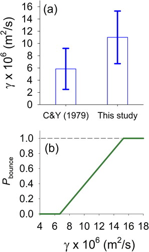
In Figure 12a, the results of this study and those of Cheng and Yeh (1979) are compared. The upper limit of $\mathrm{\gamma }$ was approximately 1.7 times the value reported by Cheng and Yeh (1979), indicating that the NaCl and LM particles generated by the IAG were less prone to bouncing than the test particles used by Cheng and Yeh (1979).

Figure 12. (a) Comparison of the particle bounce parameter, $\gamma ,$ used in this study and that used by Cheng and Yeah (1979). In this study, particle bounce was observed to occur at $\gamma$ = 6.7 × 10⁻⁶, which is the lower end of the error bar shown in the figure. Almost all particles bounced off the surface of the metal ball at $\gamma$ = 15.3 × 10⁻⁶ which is the upper end of the error bar. The particle sizes at the lower and upper end were 6.2 and 9.2 µm, respectively for $U$ set at 2.2 m/s during the measurement of particle bounce. (b) Probability of particle bounce, $P_{\mathrm{bounce}},$ as a function of $\gamma .$ $P_{\mathrm{bounce}}$ linearly increases from zero at $\gamma$ = 6.7 × 10⁻⁶ to 1 at $\gamma$ = 15.3 × 10⁻⁶.

Cheng and Yeh (1979) used particles of fluorescent organic material (Eosin Y) as the test particles and a wash-off technique to evaluate the particles collected at the different stages of a cascade impactor. Their test particles were generated by a vibrating orifice aerosol generator and contained some doublets and satellite particles, which were not as monodisperse as the particles generated by an IAG (Iida et al. 2014). In our study, a known number of particles was introduced to a collection surface and the particles that bounced off the surface were counted in situ. The wash-off technique, however, compares the mass of the fluorescent material deposited on the collection plates, interstage walls, and cascade impactor after-filter to determine the fraction of the bounced particles while assuming that the organic particles were perfectly monodisperse. The IAG-based method used in our study had a fewer number of sources of uncertainty than the wash-off technique used by Cheng and Yeh (1979); therefore, the IAG-based method has to be more accurate than the wash-off technique.

The probability density function with respect to $\mathrm{\gamma }$ is given by 1/(${\gamma }_1-{\gamma }_0$), with ${\gamma }_0$ and ${\gamma }_1$ at 6.7 × 10⁻⁶ and 15.3 × 10⁻⁶ m²/s, respectively. The probability of particle bounce, $P_{\mathrm{bounce}},$ in the case of LM and NaCl particles as a function of $\mathrm{\gamma }$ is (8) $$P_{\mathrm{bounce}}=\min \left(1,\max \left(0,\frac{\mathrm{\gamma }-{\mathrm{\gamma }}_0}{{\mathrm{\gamma }}_1-{\mathrm{\gamma }}_0}\right)\right)$$(8)

$P_{\mathrm{bounce}}$ is plotted as a function of $d_{\mathrm{a}}$ in Figure 12b. $P_{\mathrm{bounce}}$ will be zero and unity for $\mathrm{\gamma }<{\gamma }_0$ and$\mathrm{\gamma }>{\gamma }_1,$ respectively, and will linearly increase from ${\gamma }_0$ to ${\gamma }_1$ for ${\gamma }_0\le \mathrm{\gamma }\le {\gamma }_1.$

Probability of particle bounce occurring at the OPC focusing nozzle

Figure 13 shows the structure of the inlet channel of KC-31.¹⁰ The inlet channel of KC-31 has a front segment and a focusing segment. The diameter at the entrance to the front segment is 10.5 mm, which decreases to 4.9 mm at the exit of the segment or at the entrance to the focusing segment. The approximate length of the front segment is 39.2 mm¹¹; therefore, the approximate full angle of the opening is 8.2°.

Figure 13. Cross-sectional view of the inlet channel of KC-31, and the terms used in the main text to describe each part. The diameter at the entrance to the front segment, which was 10.5 mm, decreases to 4.9 mm at the exit of the front segment. The full angle of the opening is approximately 8.2°. The cross section of the focusing segment at the entrance is a circle. The cross section becomes an elongated oval at the outlet nozzle.

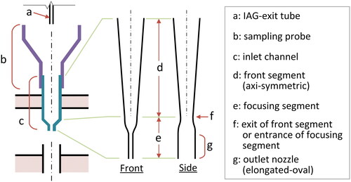
Particle bounce is expected to occur in the inner surface of the focusing segment (“e” in Figure 13). The focusing segment has a circular cross section at its entrance (“f” in Figure 13). The cross section of the inlet channel, which is initially a circle, becomes an elongated oval at the outlet nozzle (“g” in Figure 13). The transition occurs in the axial direction within 5–6 mm from “f”. The highest flow velocity was attained inside the focusing segment. Equation (7) can be used to predict the size at which particle bounce occurs in the focusing segment. To calculate $U$ using the equation $U=4Q/(\pi W^2)$ the value of $W$ is required. Once W is known, $\mathit{Stk}$ could be calculated using Equation (6)(6) $$\mathit{Stk}=\frac{4\rho Q{C}_{\mathrm{c}}{d}_{\mathrm{s}}^2}{9\pi \mu W^3}$$(6) . However, setting an appropriate value for $W$ was difficult because the dimensions in the focusing segment were not well-characterized or known. In this study, the diameter, $W_{\mathrm{e}\mathrm{q}},$ which is equivalent to the diameter of the round nozzle of the impactor used in the particle-bounce model, was set to 4.9 mm, is the diameter at the exit of the front segment of the inlet channel or at the entrance to the focusing segment (“f” in Figure 13). The value of $U$ was 25 m/s. The Reynolds number, $Re,$ which was calculated using the equation $Re=4{\rho }_{\mathrm{a}}Q/(\pi \mu W_{\mathrm{e}\mathrm{q}})$ was 8100. $Re$ > 5000 indicates a turbulent flow regime; however, the flow in the inlet channel was expected to remain stable. As Figure 2 shows, unless there is a turbulence in the environment the pulse height distribution does not broaden, indicating that the propagation of flow instability was suppressed by the converging geometry of the inlet channel. In the classifying region of a differential mobility analyzer with converging geometry, the flow remains stable even at $Re>$ 20,000 (Fernández de la Mora and Kozlowski 2013). Finally, $P_{\mathrm{bounce}}^{\mathrm{OPC}}$ was calculated as a function of$d_{\mathrm{a}}.$ The upper limit of $P_{\mathrm{bounce}}^{\mathrm{OPC}}$ could be set to ($1-{TE}_{\infty }),$ where ${TE}_{\infty }$ is the fraction of incoming particles that penetrate through the focusing segment, because the trajectories of these particles are parallel to the axial direction. ${TE}_{\infty },$ obtained by assuming that the measured CE for TFMS particles was the TE through the inlet channel, was 0.45. The details of the calculation are given in Section 3 of the SI. (9) $$P_{\mathrm{bounce}}^{\mathrm{OPC}}=(1-{TE}_{\mathrm{\infty }})\mathrm{ }\min \left(1,\max \left(0,\frac{\mathrm{\gamma }-{\mathrm{\gamma }}_0}{{\mathrm{\gamma }}_1-{\mathrm{\gamma }}_0}\right)\right)$$(9)

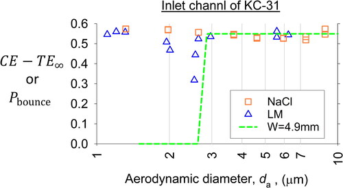
$P_{\mathrm{bounce}}^{\mathrm{OPC}}$ is plotted as a function of $d_{\mathrm{a}}$ in Figure 14. $P_{\mathrm{bounce}}^{\mathrm{OPC}}$ increases from zero to 0.55 as $d_{\mathrm{a}}$ increases from 2.6 to 2.9 µm. The figure also includes the CE of solid particles minus ${TE}_{\infty }.$ The fraction which moves in a straight line through the nozzle are subtracted from the CE to match the upper limit of $P_{\mathrm{bounce}}^{\mathrm{OPC}}.$ The size range where $P_{\mathrm{bounce}}^{\mathrm{OPC}}$ increases is slightly greater than the size range within which the CE for LM particles has a sharp minimum at $d_{\mathrm{a}}$= 2.5 µm. The results indicate that the actual value of $W_{\mathrm{e}\mathrm{q}}$ is smaller than the diameter of the focusing segment entrance (4.9 mm, “f” in Figure 13). When the CE reaches a sharp minimum, the LM particles are expected to collide with the inner surface of the focusing segment at a small angle to the surface, and the sampled particles are intercepted and captured. The depth of the dip in $CE- {TE}_{\infty }$ curve for LM particles indicates that about 23% of the sampled particles that fly off from the streamlines are captured at $d_{\mathrm{a}}$= 2.5 µm by interception. Thus, the CE observed using particle bounce models indicates that the particle deposition/bounce occurs while the flow accelerates through the focusing segment.

Figure 14. Probability of particle bounce, $P_{\mathrm{bounce}},$ at the focusing segment of KC-31 as a function of $d_a.$ The CE for solid particles less ${TE}_{\infty }$ is also shown to indicate that the size range (2.6–2.9 µm) in which $P_{\mathrm{bounce}}$ increases is slightly larger than the size where the CE of LM particles had a sharp minimum at 2.5 µm. At the sharp minimum of the CE, the LM particles are expected to collide with the inner surface of the focusing segment at a small angle to the surface; therefore, about 23% of the sampled particles would be captured by interception.

As Figure 9 shows, the CE (or $CE- {TE}_{\infty }$ Figure 14) of each of the two OPCs measured for NaCl particles remains constant when $d_{\mathrm{a}}$ is between 0.68 and 8.8 µm; therefore, the smallest size of the NaCl particles that can collide with the nozzle is not evident, unlike in the case of LM particles. Increasing the number of data points between $d_{\mathrm{a}}$ = 2.0 and 3.0 µm may cause a sharp minimum in the measured CE for the NaCl particles as well. The results of the direct-impaction experiments shown in Figure 11 demonstrate that the lower bound of the particle bounce is nearly same for LM and NaCl particles. It can be concluded that the NaCl particles that have $d_{\mathrm{a}}$ in the 2.3–2.9 µm range collide with the wall of the focusing segment and that they bounce off from the wall as the equation for $P_{\mathrm{bounce}}^{\mathrm{OPC}}$ predicts.

As shown in Figure 10, the measured CE of Solair 1100 for LM particles has a sharp minimum at an approximate particle size of 2.6 µm, and the size-dependent profile of the measured CE over the micrometer range qualitatively is same for KC-31 and Solair 1100. The solid particles having $d_{\mathrm{a}}$ larger than 2.6 µm approximately also may bounce off at the focusing segment of Solair 1100. As observed in KC-31 for NaCl particles, the measured CE of Solair 1100 did not show any significant decrease at particle sizes in the range 1–5 µm when PSL particles were used as the test aerosol particles (Figure 9). Cheng and Yeh (1979) reported that PSL particles were more prone to bouncing than organic fluorescent particles. PSL particles 2.742 and 5.067 µm in size could bounce off the surface in the focusing segment of Solair 1100.

Characteristics of large particle transport

As shown in Figure 9, the measured CEs of the OPCs for NaCl particles increase when $d_{\mathrm{o}}>$ 9 µm and reach 1.2 at $d_{\mathrm{o}}$= 12 µm. Our previous study showed that NaCl particles are agglomerates of cubic crystals (Iida et al. 2014). The apparent increase in the measured CEs could be attributed to the breaking up of the agglomerates when they collide with the wall. When NaCl particles whose $d_{\mathrm{o}}$ was 12 µm were sampled by KC-31, the differential particle count at particle sizes less than 1 µm was approximately 10 times the count when LM particles with the same $d_{\mathrm{v}}$ were sampled. Thus, NaCl particles with $d_{\mathrm{v}}$ greater than 10 µm are not suitable for use as test particles when evaluating the CE of an OPC that has a sampling flowrate of 28.3 L/min. The measured CEs of Solair 1100 and KC-31 for LM particles gradually decreased for $d_{\mathrm{o}}>$ 6.5 µm and $d_{\mathrm{o}}>$ 8.6 µm, respectively. The TE of the particles moving through the front segment (“d” in Figure 13), ${TE}_{\mathrm{front}},$ was estimated using their TE when passing through a tube with a contraction angle (Muyshondt, McFarland, and Anand 1996). The calculated ${TE}_{\mathrm{front}}$ or values of $d_{\mathrm{a}}$ larger than 2.7 µm are shown using a light green line in Figure S5. ${TE}_{\mathrm{front}}$ follows the size dependence of the CE for LM particles indicating that LM particles with $d_{\mathrm{a}}>$ 10 µm are lost through the front segment of the inlet channel; however, the CE systematically exceeds ${TE}_{\mathrm{front}},$ suggesting that some fraction of LM particles will bounce off the surface of the front segment.

Conclusion

This study investigated the effect of particle phase on the CEs of the OPCs KC-31 and Solair 1100 at a sampling flowrate of 28.3 L/min. The CEs were evaluated at particle sizes ranging from 0.3 to 10 µm. Solid (LM and NaCl) and liquid (TFMS) particles were generated at a constant rate using an IAG. PSL particles, 1.0, 2.7, and 5.1 µm in size, also were used to evaluate the CE of Solair 1100. Overall, the dependence of the two OPCs on the size and material of the particles were similar for sizes in the range 1–10 µm. In the case of liquid particles the CEs starts decreasing at sizes larger than 1–2 µm, then at sizes larger than 5 µm, the CEs were between 0.3 and 0.5. The CE of each of the OPCs had a sharp minimum when the LM particle size was in the 2.5–2.6 µm range. At sizes beyond the 3–4 µm range, the CE for LM particles was in the range 0.95–1.0. This trend indicates that LM particles of sizes larger than a few micrometers bounce off the surface of the front segment, whereas the TFMS particles in the same size range deposit on the surface. The particle deposition/bounce can occur while the flow accelerates through the focusing segment of the inlet channel. To prove this hypothesis, particle transport models for particle bounce were used. The probability of particle bounce in solid particles, which is a function of $\mathrm{\gamma }$ ($=U_{\mathrm{i}}{d}_{\mathrm{a}}$), was evaluated using additional experiments. The mathematical relationship for particle bounce was thereafter used to predict the size range in which the probability of particle bounce would increase at the focusing nozzle. This size range was between 2.6 and 2.9 µm and was slightly larger than the size at which the CE for LM particles had a sharp minimum (d_a = 2.5 µm). This minimum could be the particle size at which the angle between the trajectory of incoming LM particles and the wall surface was minimum, which would have enabled the particles to intercept the surface. Some of these intercepting particles would have been captured. The CE for the NaCl and PSL particles did not show any significant decrease over a few micrometer range. However, considering that the probability of particle bounce is similar for NaCl and LM particles and that PSL particles also are prone to bounce, it can be concluded that both NaCl and PSL particles would have bounced off at the focusing nozzle of the OPCs.

The airborne particle number over the micrometer range, often considered the surrogate of biological particles in pharmaceutical environments, is monitored in cleanroom environment. The physical state of particles containing microorganisms can be diverse; the microorganisms can be a part of crystals, fibers, or liquid particles. OPC users in the pharmaceutical field should be aware that the TE of the particles passing through the inlet channel of an OPC with a sampling flowrate of 28.3 L/min is significantly affected by the physical state of the sampled particles.

Nomenclature

Symbols

$C_{\mathrm{c}}$	=	slip correction factor
$C_{\mathrm{m}}$	=	concentration of the solute in each inkjet solution, mass of solute/mass of solution
CE	=	counting efficiency of an OPC defined as the ratio of the particle count rate of the OPC to the particle generation rate of the IAG
DF	=	detected fraction, the fraction of incoming particle detected by KC-31 at downstream of a metal-impaction ball
$d_{\mathrm{a}}$	=	aerodynamic diameter of aerosol particles, m.
$d_{\mathrm{o}}$	=	optical diameter, the diameter of PSL particles when the intensity of the scattered light is equal to that of the test particles generated by the IAG, m
$d_{\mathrm{s}}$	=	Stokes diameter of aerosol particles, m
$d_{\mathrm{v}}$	=	volume equivalent diameter of aerosol particles, m
$d_{50}$	=	particle diameter at which the size dependent penetration curve reaches 50%, m
$f_{\mathrm{d}}$	=	droplet generation rate of an inkjet head, s−1
$L_{\mathrm{IAG}}$	=	particle generation rate of an IAG, s−1
$L$	=	particle count rate of an OPC, s−1
${\overline{L}}_{\mathrm{plug}},$ ${\overline{L}}_{\mathrm{parablic}}$	=	value of $L$ averaged over multiple measurements. During these measurements, test particles are delivered to simulate particle flux in plug flow and parabolic flow, respectively, s−1
$\overline{L}$	=	expected particle count rate, which is the weighted average of ${\overline{L}}_{\mathrm{plug}}$ and ${\overline{L}}_{\mathrm{parablic}}$ assuming that the most probable velocity profile over the inlet plane is plug flow, s−1
$N$	=	number of particles detected by an OPC
$P_{\mathrm{bounce}}$	=	probability of particle bounce as a function of $\mathrm{\gamma }$ for the solid particles at a metal surface
$P_{\mathrm{bounce}}^{\mathrm{OPC}}$	=	probability of particle bounce at the focusing nozzle of an OPC
$Q$	=	flowrate through the nozzle of an impactor, m3/s
$Q_{\mathrm{cham} }$	=	flowrate through the sheath flow chamber, m3/s
$r$	=	radial distance from the center axis of the sampling probe, m
$R$	=	inner radius of the sampling probe, m
$Re$	=	Reynolds number of flow through a circular tube
$\mathit{Stk}$	=	Stokes number of aerosol particles.
${\mathit{Stk}}_{50}$	=	$\mathit{Stk}$ at which the deposition efficiency of an impactor is 50%, m
$t$	=	sampling time of an OPC, s
${TE}_{\mathrm{front}}$	=	transport efficiency through the front segment of the inlet channel
$U$	=	average flow velocity at the nozzle of an impactor, m/s
$U_i$	=	particle velocity when a particle impacts on a substrate, m/s
$u\left(x\right)$	=	standard uncertainty of the uncertainty factor $\mathrm{x}$
$u_{\mathrm{rand}}\left(x\right), u_{\mathrm{sys}}\left(x\right)$	=	random and systematic components of the standard uncertainty, respectively.
$W$	=	nozzle diameter of an impactor, m
$W_{\mathrm{e}\mathrm{q}}$	=	equivalent nozzle diameter, the diameter which is equivalent to that of a round nozzle of an impactor in the particle-bounce model, m
$W_{\mathrm{cham}}$	=	inner diameter of the sheath flow chamber, m
$\Gamma$	=	threshold value of $\mathrm{\gamma }$ above which the particle bounce is expected to occur, ${10}^{-6}$ m2/s
$\mathrm{\gamma }$	=	the parameter which controls the particle bounce, $U_i{d}_{\mathrm{s}}\sqrt{\rho /{\rho }_0},$ m2/s
$\mu$	=	dynamic viscosity, Pa⋅s
$\rho$	=	material density of the particle material, kg/m3
${\rho }_{\mathrm{a}}$	=	density of air, kg/m3
${\rho }_0$	=	unit density, 1 g/cm3 or 1000 kg/m3
$\mathrm{\psi }\left(L\right)$	=	probability density function of the particle count rate, s

Abbreviations
ANOVA	=	analysis of variance
APS	=	aerodynamic particle sizer
CE	=	counting efficiency
DEMC	=	differential electrical mobility classifier
DF	=	detected fraction
DUT	=	device under test
IAG	=	inkjet aerosol generator
LM	=	lactose monohydrate
PHA	=	pulse height analysis
TE	=	transport efficiency
TFMS	=	1-ethyl-3-methylimidazolium trifluoromethanesulfonate

Acknowledgement

This work was partly carried out under “Budget for promotion of strategic international standardization” commissioned by Ministry of Economy, Trade and Industry (METI), Japan.

Notes

1 The speed of filtered air in a laminar flow system should be in the range 0.36–0.54 m/s. The diameter of the sampling probe was 33 and 41 mm when the sampled air passed through the probe at 0.54 and 0.36 m/s, respectively.

2 The inner and outer diameters of the IAG exit tube were 3.18 mm and 1.74 mm, respectively. The inside of the tube was tapered.

3 Aerosol particles were expected to uniformly mix in the sampling environment; therefore, the particle number concentration (particles m⁻³) was assumed to be constant. The particle flux (particles m⁻² s⁻¹) over the inlet plane as a function of the radial distance from the center is linearly proportional to the axial flow velocity (m s⁻¹) because particle flux is the product of the particle number concentration and velocity.

4 The program spent 15 seconds at each point, and the particle generation rate of the IAG was set at 30.00 s⁻¹; thus, 450 particles were delivered to each point. On average, approximately 12% of the sampling time was taken by the particles to move through the 32 points.

5 Measurement points over the inlet plane of the sampling probe were equally spaced in the radial and angular directions, excluding the center. There were 8 and 24 measurement points in the radial and angular directions, respectively.

6 The CE for NaCl particles were measured about 1 to 1.5 years later. At that time the demo unit had been returned to its manufacturer, and the measurements were done using a commercial version.

7 The interpolation was performed on a log-log scale.

8 The inkjet process generated several satellite droplets when isopropyl alcohol was used as the dispersion medium; therefore, the average mass of a droplet was unknown.

9 The corresponding values of $\sqrt{Stk}$ at 6.2 μm and 9.4 μm were 0.67 and 0.98, respectively, which are both higher than $\sqrt{{\mathit{Stk}}_{50}}.$

10 NMIJ has a KC-31 OPC; therefore, the inlet channel could be temporarily removed from the optical components to view the structure of the inlet channel. Because Solair 1100 is used as a transfer standard at METAS, its inlet channel could not be removed to view its structure.

11 The exit diameter and length of the front segment of the inlet channel of KC-31were measured by inserting the back side of a drill bit into the inlet channel.

References

- Bohren, C. F., and D. R. Huffman. 1998. Absorption and scattering by a sphere. In Absorption and scattering of light by small particles, 82–129. Weinheim, Germany: Wiley-VCH Verlag GmbH & Co. KGaA.
- Borggräfe, P., A. Trampe, and H. Fissan. 2002. Quantitative characterization of noise in the measurement chain of an optical particle counter. Meas. Sci. Technol. 13:445–50.
- Chen, B. T., H. C. Yeh, and Y. S. Cheng. 1985. A novel virtual impactor: Calibration and use. J. Aerosol Sci. 16 (4):343–54. doi:10.1016/0021-8502(85)90042-4.
- Cheng, Y.-S. and H.-C. Yeh. 1979. Particle bounce in cascade impactors. Env. Sci. Technol. 13:1392–6. doi:10.1021/es60159a017.
- CRC. 2013. Section 4: Properties of the elements and inorganic compounds. In CRC handbook of chemistry and physics, 93rd edition (DVD version 2013), ed. W. Haynes. Boca Raton, FL: CRC Press/Taylor and Francis.
- Fernández de la Mora, J., and J. Kozlowski. 2013. Hand-held differential mobility analyzers of high resolution for 1–30nm particles: Design and fabrication considerations. J. Aerosol Sci. 57:45–53. doi: 10.1016/j.jaerosci.2012.10.009.
- Horender, S., K. Auderset, and K. Vasilatou. 2019. Facility for calibration of optical and condensation particle counters based on a turbulent aerosol mixing tube and a reference optical particle counter. Rev. Sci. Instrum. 90 (7):075111. doi: 10.1063/1.5095853.
- Iida, K., and H. Sakurai. 2018. Counting efficiency evaluation of optical particle counters in micrometer range by using an inkjet aerosol generator. Aerosol Sci. Technol. 52 (10):1156–11. doi: 10.1080/02786826.2018.1505032.
- Iida, K., H. Sakurai, K. Saito, and K. Ehara. 2014. Inkjet aerosol generator as monodisperse particle number standard. Aerosol Sci. Technol. 48 (8):789–802. doi: 10.1080/02786826.2014.930948.
- ISO/TC24/SC4/WG3. 2014. Determination of density by volumetric displacement—Skeleton density by gas pycnometry. Geneva, Switzerland: International Organization for Standardization.
- ISO/TC24/SC4/WG9. 2018. ISO 21501-4: Determination of particle size distribution – Single particle light interaction methods – Part 4: Light scattering airborne particle counter for clean spaces. Geneva, Switzerland: International Organization for Standardization.
- Katayama, H., K. Yoshihara, H. Saito, M. Akutagawa, A. Okamoto, R. Okamoto, M. Kaneko, Y. Kawakita, M. Kamitani, R. Gotoda, et al. 2012. Evaluation of rapid microbiological method for airborne bacterium. PDA J. GMP Valid. Japan 14:43–7. doi: 10.11347/pda.14.43.
- Kawai, M., T. Ichijo, Y. Takahashi, M. Noguchi, H. Katayama, O. Cho, T. Sugita, and M. Nasu. 2019. Culture independent approach reveals domination of human-oriented microbes in a pharmaceutical manufacturing facility. Eur. J. Pharm. Sci. 137:104973. doi: 10.1016/j.ejps.2019.104973.
- Kerker, M. 1969. The scattering of light and other electromagnetic radiation: Academic Press.
- Kesavan, J., J. R. Bottiger, and A. R. McFarland. 2008. Bioaerosol concentrator performance: Comparative tests with viable and with solid and liquid nonviable particles. J. Appl. Microbiol. 104 (1):285–95. doi: 10.1111/j.1365-2672.2007.03560.x.
- Le, T.-C., and C.-J. Tsai. 2021. Inertial impaction technique for the classification of particulate matters and nanoparticles: A review. KONA 38:42–63. doi: 10.14356/kona.2021004.
- Malli Mohan, G. B., M. C. Stricker, and K. Venkateswaran. 2019. Microscopic characterization of biological and inert particles associated with spacecraft assembly cleanroom. Sci. Rep. 9 (1):14251. doi: 10.1038/s41598-019-50782-0.
- Marple, V. A., and B. A. Olson. 2011. Sampling and measurement using inertial, gravitational, centrifugal, and thermal techniques. In Aerosol measurement, ed. P. Kulkani, P. A. Baron, and K. Willeke, eds., 3rd ed., 129–51. Hoboken, NJ: John Wiley & Sons, Inc.
- Marple, V. A., K. L. Rubow, and S. M. Behm. 1991. A microorifice uniform deposit impactor (moudi): Description, calibration, and use. Aerosol Sci. Technol. 14 (4):434–46. doi: 10.1080/02786829108959504.
- Minakami, T., T. Hosokawa, K. Kondo, K. Iida, K. Ehara, and H. Sakurai. 2017. Evaluation of counting efficiencies for optical particle counters by using inkjet aerosol generator. Earozoru Kenkyu 32:29–36. doi: 10.11203/jar.32.29.
- Muyshondt, A., A. R. McFarland, and N. K. Anand. 1996. Deposition of aerosol particles in contraction fittings. Aerosol Sci. Technol. 24 (3):205–16. doi: 10.1080/02786829608965364.
- Sachweh, B., H. Umhauer, F. Ebert, H. Büttner, and R. Friehmelt. 1998. In situ optical particle counter with improved coincidence error correction for number concentrations up to 107 particles cm − 3. J. Aerosol Sci. 29 (9):1075–86. https://doi.org/10.1016/S0021-8502.(98)80004-9. doi: 10.1016/S0021-8502(98)80004-9.
- Sang-Nourpour, N., and J. S. Olfert. 2019. Calibration of optical particle counters with an aerodynamic aerosol classifier. J. Aerosol Sci. 138:105452. doi: 10.1016/j.jaerosci.2019.105452.
- Tran, S., K. Iida, K. Yashiro, Y. Murashima, H. Sakurai, and J. S. Olfert. 2020. Determining the cutoff diameter and counting efficiency of optical particle counters with an aerodynamic aerosol classifier and an inkjet aerosol generator. Aerosol Sci. Technol. 54 (11):1335–10. doi: 10.1080/02786826.2020.1777252.
- Vasilatou, K., K. Dirscherl, K. Iida, H. Sakurai, S. Horender, and K. Auderset. 2020. Calibration of optical particle counters: First comprehensive inter-comparison for particle sizes up to 5 µm and number concentrations up to 2 cm − 3. Metrologia 57 (2):025005. doi: 10.1088/1681-7575/ab5c84.
- Volckens, J., and T. M. Peters. 2005. Counting and particle transmission efficiency of the aerodynamic particle sizer. J. Aerosol Sci. 36 (12):1400–8. doi: 10.1016/j.jaerosci.2005.03.009.
- Yli-Ojanpera, J., H. Sakurai, K. Iida, J. M. Makela, K. Ehara, and J. Keskinen. 2012. Comparison of three particle number concentration calibration standards through calibration of a single cpc in a wide particle size range. Aerosol Sci. Technol. 46 (11):1163–73. doi: 10.1080/02786826.2012.701023.