Analytical challenges when sampling and characterising exhaled aerosol

Abstract

Respiratory particles produced by breathing, coughing, and speaking or generated during medical procedures serve as important routes for disease transmission. Characterizing the number of particles generated as well as their size distribution is fundamental for guiding policy on infection control. However, sampling such particles carries inherent challenges. Respiratory particles are polydisperse in size, temporally and spatially variable, and emitted in very low concentrations, usually lower than the preexisting aerosol concentration in indoor environments. In addition, they are typically emitted in a highly dynamic, warm and humid jet, leading to further rapid processes, such as dispersion and evaporation. Here, we discuss important considerations for sampling respiratory aerosol, focusing on sampling particles <20 μm in diameter. Instruments capable of counting single-particles within this size range are commercially available. We provide recommendations for experimental protocols and demonstrate the limitations behind such approaches. We highlight the importance of a measurement space with as low a background aerosol concentration as possible, and of sampling for as long as possible to enable accurate quantitation of the size distribution of an aerosol plume. This is particularly important for the larger particles (>5 μm diameter) that are so low in concentration that they may require hours of sampling time to be accurately quantified. We explore the relationship between the flow rates of the exhalation and the sampling instrument and the consequent quantification of particle flux. We also discuss the transport and evaporation dynamics of liquid particles within respiratory jets, and their impacts on conducting aerosol sampling studies.

EDITOR:

• Pramod Kulkarni

1. Introduction

An accurate representation of the concentrations (both number and mass) and size distributions of exhaled aerosol particles and droplets is fundamental to our understanding of the spread of infectious respiratory pathogens. The airborne and droplet modes of transmission have been shown to be key for many pathogens, including influenza (Herfst et al. 2012), measles, tuberculosis (Tellier et al. 2019) and severe acute respiratory syndrome coronavirus (SARS-CoV-1) (Li et al. 2005), and are now considered important in the transmission of SARS-CoV-2. Early in the coronavirus disease (COVID-19) pandemic, serious concerns arose around certain activities thought to generate large concentrations of respiratory aerosol with the potential to enhance the risk of airborne transmission. For example, in the performing arts industry, singing and playing wind instruments in public were prohibited. In healthcare settings, medical procedures thought to release airborne particles, known as Aerosol Generating Procedures (AGPs), could only proceed with the use of high levels of personal protective equipment (PPE) and, in some cases, reduced staff attendance, as well as with ‘fallow times’ to allow sufficient time for aerosol to dissipate between procedures. (Hamilton et al. 2021a; Hamilton et al. 2021b; Brown et al. 2020).

Different strategies have been employed to identify which activities or medical procedures pose a significant risk of viral transmission from an infected individual to a susceptible one (e.g., participants, audience, or healthcare workers). First, retrospective epidemiological studies allow identification of ‘spreading events’ by tracing new infections (Charlotte 2020; Tran et al. 2011). Second, microbiological techniques have been used to sample indoor air at high volumetric flow rate onto gelatin media or directly into liquid media, followed by quantification of virus by reverse transcription polymerase chain reaction (RT-PCR, for RNA copy number) or plaque assay (for infectious virus) (Ratnesar-Shumate et al. 2021). This approach has identified the presence and survival of SARS-CoV-2 virus in hospitals (Lednicky et al. 2020; Liu et al. 2020). However, direct identification and quantification of airborne infectious pathogens is challenging and not always tractable. A third approach to assess the potential risk of disease transmission is to quantify aerosols and droplets, the vehicles for transporting an infectious pathogen, generated from the human respiratory tract during normal respiratory activities like coughing (Hamilton et al. 2021b; Johnson et al. 2011; Morawska et al. 2009), breathing (Almstrand et al. 2010; Holmgren et al. 2010), speaking (Asadi et al. 2019) and singing (Gregson, Watson, et al. 2021; Mürbe et al. 2020; Alsved et al. 2020), as well as originating from aerosol generating procedures (Wilson et al. 2021; Brown et al. 2020; Gaeckle et al. 2020). Although not identifying the presence of infectious pathogens or quantifying loadings, these measurements can provide important insights to help guide public health policy.

The detection of aerosols and droplets originating from the human respiratory tract, either through expiratory activities like coughing, speaking or breathing, or arising during medical procedures presents inherent measurement challenges. The current state of knowledge on respiratory aerosol has been reviewed in detail elsewhere (Pöhlker et al. 2021); we limit our discussion and analysis to the challenges associated with performing respiratory aerosol measurements. Although there is no “perfect” sampling methodology or instrument, and observational sampling studies during a pandemic will likely have to work around serious constraints (space, time, instrument availability), we provide an assessment of how aerosol generated from respiratory activities can be robustly attributed and quantified. In particular, four properties of respiratory aerosol present particular measurement challenges, as summarized in Figure 1. We begin by summarizing these challenges.

Figure 1. (a) Schematic figure depicting important properties of respiratory aerosol emissions and resulting methodological challenges for sampling studies discussed in this work. (b) The size distribution of aerosol 0.3 – 500 µm diameter generated by a cough, demonstrating polydispersity in size (Johnson et al. 2011).

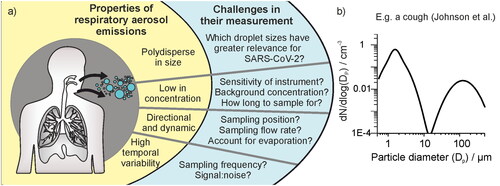
Particles generated and exhaled from the respiratory tract span a wide range in size from several nanometers up to hundreds of micrometers. Particles smaller than 10 μm in aerodynamic diameter can be inhaled into the human respiratory tract, and those smaller than 2.5 μm can even enter the deep lung and alveoli. For coughing and speaking, Johnson and Morawksa have reported generation of a trimodal size distribution (Johnson et al. 2011; Morawska et al. 2009). The largest “droplet” mode consists of ∼20 μm – >1000 μm diameter droplets and is generated within the oral cavity. Fine respirable aerosols are described by two overlapping lognormal size distributions spanning ∼0.1–20 μm diameter, one generated within the alveoli and the other generated by vibrations in the larynx (Figure 1b). In disease transmission, it is common to talk about droplet and airborne modes of transmission, arising from the droplet and aerosol modes, respectively. However, this delineation has been challenged, as a particle 20–100 μm is not so dissimilar in its aerodynamic transport to much smaller respirable aerosols and can be transported over medium distances (Bourouiba 2021; Prather et al. 2020; Vuorinen et al. 2020). Thus, particles <100 μm require different strategies for infection control (e.g., improved ventilation and respirator masks) to those larger than 100 μm that follow ballistic trajectories, for which physical distancing is the prime mitigation strategy. We refer to any particle smaller than 100 μm in diameter as an aerosol particle in our discussion below.

Common with many aerosol measurements, identifying a single technique that covers the entire polydisperse size range is impossible. Aerodynamic, optical and electric mobility sizers have been used to characterize the respirable sized aerosols below 10 μm in diameter although any one of these cannot cover the size range 10 nm to 10 μm entirely. Instead, recognizing the physical size of most pathogens (i.e., ∼100 nm for SARS-CoV-2, (Bar-On et al. 2020)) and the increasing likelihood that individual particles can be “empty” (i.e., do not contain even a single virus) with diminishing particle size even at high viral titer, it is appropriate and convenient to concentrate measurements on particles larger than 300 nm with optical and aerodynamic particle sizers. There is currently a pressing need to develop methods to sample 10–100 μm diameter particles. The concentrations of these larger particles, arising from the upper respiratory tract and oral cavity (Johnson et al. 2011), are exceptionally challenging to quantify. If the load or dose of a pathogen within a droplet scales with respiratory fluid mass, then this size range could dominate the mass fraction despite accounting for only a tiny fraction of the number concentration. (This assumption may not always be valid: for instance, evidence suggests that for some diseases like influenza, a higher viral load may preferentially be found in smaller particles (Yan et al. 2018)). Approaches to quantify the larger (>20 μm) particles include imaging using high-speed cameras (Alsved et al. 2020), laser sheet imaging (Stadnytskyi et al. 2020), imaging deposited respiratory droplets doped with fluorescent dyes (Llandro et al. 2021; Newsom et al. 2021; McGhee et al. 2020), or using water sensitive paper (McCarthy et al. 2021).

Respiratory aerosol has a low number concentration. Previous work has aimed to quantify the concentration of aerosol generated from expiratory activities within the exhalation flow (Gregson, Watson, et al. 2021; Alsved et al. 2020; Asadi et al. 2019; Johnson et al. 2011). Reporting the intensive property of sampled concentration has allowed such studies to compare a relative aerosol yield generated by different types of respiratory activity. These studies demonstrate that generated aerosol concentrations are typically much lower (∼ 0.1–10 cm⁻³ (Gregson, Watson, et al. 2021)) than the preexisting background aerosol concentration in most indoor environments, which can generally range from 100 s–1000s cm⁻³ (Vette et al. 2001). Such low concentrations of respiratory aerosol require measures to either reduce the preexisting aerosol concentration for reliable sampling, or accurately quantify it for background subtraction. There is a large interpersonal variability in the aerosol concentration generated by respiratory activities and therefore a large cohort of subjects is required to accurately assess a mean concentration. (Gregson, Watson, et al. 2021; Asadi et al. 2019).

Respiratory aerosol flux is often transient, and always temporally variable. Respiratory activities vary widely in their duration, spanning transient activities like coughing or sneezing, to activities with quantifiable durations like breathing, speaking, and singing but with highly variable flow rates and complex temporal cycles. Consequently, robust measurement requires use of instrumental approaches with high time resolution (e.g., 1 s). In addition, respiratory aerosol is dynamic and directional when first exhaled, and spatially heterogeneous. The high surface area-to-volume ratio of respiratory particles allows rapid equilibration with their surrounding gas phase, leading to fast changes in droplet size and phase (Walker et al. 2021). From coughs and sneezes, the aerosol is emitted in a multiphase turbulent jet and there are steep jet velocity and aerosol concentration gradients with changing position relative to the source (Bourouiba, Dehandschoewercker, and Bush 2014). Owing to dispersion and dilution, signal from these activities is spatially heterogeneous. Aerosol generated by a point source in a room will rapidly dilute as the particles mix with the surrounding environment, leading to even greater challenges in detecting and quantifying respiratory aerosol at increasing distance from the human source.

We provide an assessment of the current frameworks for measuring and reporting aerosol fluxes from respiratory activity below, along with new data and analyses to highlight the challenges of quantification. We introduce the methods used for the new data reported here in Section 2. In Section 3 we consider the role of background aerosol and noise, the volumetric flow rates of the detection instruments used, the required acquisition times for accurate characterization of particle size distributions, the dynamic changes in respiratory aerosol size on exhalation, the ambiguities in attributing aerosol source, and intersubject variability and cohort size.

2. Materials and methods

For the measurements reported in this publication, aerosol number concentrations and size distributions were sampled using either an optical particle sizer (OPS, model 3330 from TSI, USA, sampling particles 0.3 − 10 μm diameter, flow rate 1 L min⁻¹) or an aerodynamic particle sizer (APS, model 3321 from TSI, USA, sampling particles 0.5 − 20 μm diameter, sample flow rate 1 L min⁻¹ with sheath flow rate 4 L min⁻¹). The aerosol instrument used for each measurement (APS or OPS) and other sampling details such as sampling location are specified when reporting the measurement results.

Data for exhaled aerosol concentrations sampled from a single human subject are presented in Figures 2 and 4. The data in Figure 2 were collected following ethical approval granted by the Greater Manchester REC committee (Reference: 20/NW/0393) as part of the AERATOR study (approved 18/09/2020). The study is registered in the ISRCTN registry (ISRCT:N21447815) and was granted Urgent Public Health status by the NIHR. The data in Figure 4 were collected following ethical approval granted by the PHE Research Ethics and Governance Group as part of the PERFORM study (Reference: R&D 429, approved 10/02/2021).The protocol for collecting exhaled aerosol concentrations in Figures 2 and 4 is the same as in Gregson et al. and so will only be reviewed briefly here (Gregson, Watson, et al. 2021). A subject positioned their face directly into a 3 D-printed polylactic acid funnel (15 cm cone diameter) and the aerosol concentration in their exhaled air was sampled by an APS or OPS connected to the funnel by 1 m conductive silicone tubing (TSI, model 3001788, inner diameter 0.19 inch, outer diameter 0.375 inch).

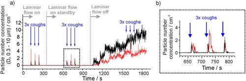
Figure 2. (a) Aerosol number concentration in a laminar flow operating theater measured with an OPS when a subject produces a voluntary cough at defined times (indicated by the blue arrows). The laminar flow in the theater is initially on, turned to standby mode at 360 s, and turned off completely at 1020 s. In both black and red data sets (two data collections), aerosol generated by a cough is clearly detected above the background concentration when the laminar flow system is on or in standby mode, but not when the laminar flow has been turned off for 8 min. (b) Expanded view of three coughs from the two data collections in a) when the laminar flow system is on standby.

3. Results and discussion

3.1. Background aerosol concentration and noise

Quantifying the aerosol concentration generated by different activities requires the aerosol concentration in the exhalation plume to be identifiable above a background aerosol concentration that is steady over the course of the measurement. Thus, the environment in which such measurements are made must be carefully considered. The importance of a low background is illustrated in Figure 2. An orthopedic operating theater with a laminar flow system (EXFLOW 32; Howorth Air Technology, Farnworth, UK, 500 − 600 air changes per hour) is an ideal space to unambiguously identify and quantify aerosol generated by a voluntary cough from a patient, as the background aerosol number concentration is close to zero particles cm⁻³ (recorded by an OPS) (Gregson, Watson, et al. 2021; Brown et al. 2020). The laminar flow system inside the orthopedic operating theater is progressively switched from on (maximum air changes per hour), to standby (25 air changes per hour), to off over several minutes. In two similar experiments, the background aerosol number concentration is shown to increase from ∼0 cm⁻³ to 4–10 cm⁻³ after the laminar flow is off for ten minutes. The respiratory aerosol generated by a single subject coughing three separate times into a sampling funnel connected to the OPS can be clearly detected above the background concentration when the laminar flow system is on or on standby (Shrimpton, Gregson, Brown, et al. 2021). However, the higher (and highly variable) aerosol background that results when the laminar flow system is switched off hinders observation of the respiratory aerosol generated ∼1500s in the experiment.

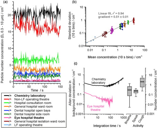
Low noise in the background aerosol concentration is required to ensure respiratory aerosol can be clearly identified. Aerosol number concentrations, sampled with a 1 s acquisition time over 150 samples (i.e., 150 individual concentration measurements), are compared in Figure 3a over several clinical or laboratory spaces. For the datasets in Figure 3a, the standard deviation of the measured number concentration over 10 samples increases with increasing mean number concentration (Figure 3b), consistent with expectations for the measured aerosol concentration following a normal distribution. Peaks of aerosol concentration generated by coughing are short lived, and therefore increased background noise will lead to increasing challenges discerning a true signal above the noise as the acquisition time increases. Methods to reduce background concentrations to conduct respiratory aerosol measurements include using HEPA filtered clean air (Asadi et al. 2019) or portable filtration systems (Hamilton et al. 2021b). To identify if the background concentration and noise in an experimental setting is sufficiently low to detect sensitively aerosol generated by an AGP, normal respiratory activities like coughing and breathing have been used as references (Gregson, Shrimpton, et al. 2021; Wilson et al. 2021; Brown et al. 2020).

Figure 3. (a) The sampled background aerosol number concentration, (OPS, D_P 0.3–10 µm), in different settings, sampled once per second for 150 samples. (b) The standard deviation from 10 s bins of the background aerosol concentration in each site shown in (a) compared to the mean concentration. (c) Allan deviation analysis on the background aerosol concentration in a chemistry lab (mean concentration ∼21 cm⁻³) and in an eye hospital theater (mean concentration ∼ 0.6 cm⁻³) compared on the same scaling to a box and whisker plot showing the number concentration generated by a cohort of 25 healthy subjects breathing, speaking or coughing (data from Gregson, Watson, et al. 2021). Whiskers represent the range (1.5IQR), boxes represent 25%–75% and bold line is the median concentration.

3.1.1. Identifying an appropriate averaging time to account for background noise

Allan deviation analysis can be used to identify an appropriate averaging time to optimize signal retrieval above a noisy background. The Allan deviation is the average standard deviation for a dataset at a varying integration time. By using the background aerosol concentration as the signal, the optimal measurement period to minimize the contribution of the background aerosol to the measurement can be identified (i.e., the time over which the noisy background is most accurately quantified allowing discrimination and quantification of an increase in signal level above the background from a respiratory activity). Figure 3c compares the Allan deviation analysis for two different measurement spaces. Initial improvements in background signal quantification are observed with increasing acquisition time but are eventually compromised by longer-term environmental drift (e.g., activities within the room, outdoor aerosol concentrations altering those indoors) that drive significant variations in the background concentration. By this acquisition time, the accuracy and appropriateness of reporting the background using a single concentration value is compromised.

Determination of the aerosol background number concentration in a chemistry laboratory (mean concentration of ∼21 cm⁻³, Figure 3a) improves with a gradual reduction in the level of noise from ±1.46 cm⁻³ to less than ±1 cm⁻³ as the acquisition time increases from 1 s to 50 s integration time (Figure 3c). Similarly, increasing the acquisition time from 1 s to 50 s in the eye hospital reduces the uncertainty in the background number concentration from ±0.16 cm⁻³ to ±0.02 cm⁻³. In both cases, increasing the acquisition time beyond ∼50–100 s leads to a degradation in the quantification of the background aerosol, a consequence of other environmental drivers that are leading to coarse changes in the background concentration that surpass the short-time fluctuations.

Box and whisker plots showing the mean aerosol number concentration sampled during different respiratory activities, from a cohort of 25 subjects, are also shown in Figure 3c (box and whisker data are plotted from Gregson, Watson, et al. 2021) for comparison with the Allan deviation characterization of the background aerosol concentration. Improvements in the characterization of the background concentration by increasing the acquisition time bring benefits to the detection of certain classes of respiratory aerosol. In the eye hospital, the aerosol generated by coughs would always be observable above the background and increasing the sampling integration time could allow detection of aerosol from even the lowest emitters during breathing and speaking. By contrast in the chemistry laboratory, the aerosol from breathing and speaking will never be quantifiable because the noise associated with the background concentration determination is always greater than the concentration generated by these respiratory activities regardless of the integration time. Note that these measurements are performed as close to the source (i.e., the mouth) as possible to minimize dispersion and dilution of the exhaled aerosol plume. In principle, some coughs may be observable above the background. However, the duration of the respiratory emission must far exceed the integration time to be observable, and because a cough is a single transient event, increasing sample integration time will not facilitate its measurement. In short, consideration of background integration highlights the necessity of a low background aerosol concentration for accurate sampling of respiratory emissions.

3.2. Volumetric flow rate of sampling instrumentation and exhaled airflow

Respiratory aerosol is exhaled within an airflow at a flow rate that varies according to the type of activity. For example, tidal breathing typically forms a sinusoidal function with a minute ventilation rate of ∼ 6 L min⁻¹ (Carroll 2007), whereas the airflow from a cough can exceed peak flow rates of 400 L min⁻¹ (Mellies and Goebel 2014). The relationship between the exhalation flow rate into a sampling volume and the sampling flow rate is important to quantify accurately aerosol flux. As illustrated in Figure 4a (Case 1), an aerosol plume exhaled into a sampling funnel at a rate greater than the volumetric flow rate drawn from the funnel leads to a steady state concentration within the funnel. Under these circumstances, only the intensive property of aerosol concentration in the exhaled air can be reported. In this limiting case, if the exhalation flow rate can be measured, the measured number concentration can be converted into an absolute number of particles emitted. Alternatively, when the volumetric sampling rate is greater than the expected flow rate of the exhaled airflow, all particles can be detected by the instrument and, thus, the extensive property of absolute number of particles generated can be reported (Figure 4a, Case 2); in this case, a measured concentration is convoluted with the additional required airflow leading to dilution and the concentration cannot be determined. In both cases, the possible loss of particles in the sampling line and a detection efficiency below 100% must be considered (Volckens and Peters 2005).

Figure 4. (a) Schematic depicting the importance of understanding the sampling flow rate relative to the exhalation rate, if sampling into a fixed volume such as a funnel, as the relationship between the two flow rates defines whether the concentration of aerosol particles or an absolute number of particles can be reported. (b) The number concentration sampled from an APS through a funnel when a subject sings at 90 – 100 dB for 10 s intervals, as the sampling flow rate is increased sequentially from 5 to 25 L min⁻¹. (c) The number concentration sampled by an APS when a subject breathed into a funnel for 60 s, as the sampling flow rate is increased from 5 to 20 L min⁻¹. Error bars report the standard error of the mean.

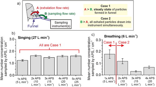
We demonstrate the importance of understanding the relationship between sampling and exhalation flow rates, using singing and breathing as examples in Figures 4b and c. A single subject sang at a sound pressure of 90–100 dB into a sampling funnel for multiple 10 s intervals and the mean aerosol number concentration in the exhalation flow was measured (the same protocol as for Gregson, Watson, et al. 2021). The aerosol number concentration was recorded by up to five APS instruments drawing exhaled flow from the sampling funnel in tandem, each drawing at 5 L min⁻¹. The sampling flow rate from the funnel was progressively increased from 5 L min⁻¹ to 25 L min⁻¹ by sequentially including additional APS instruments to draw from the funnel. The participant’s exhalation flow rate was measured separately using a cardiopulminary exercise testing (CPET) mask while the participant sang at 90–100 dB for 60 s. Because the exhalation flow rate (27.8 ± 0.2 (SD) L min⁻¹) was always larger than the total sampling flow rate (up to 25 L min⁻¹), the mean number concentration sampled by APS-1 (which always sampled from the funnel) remained relatively constant at 1.5 ± 0.2 (SD) cm⁻³ (Figure 4b). This experiment was clearly within the regime of a steady state concentration in the funnel (Case 1 in Figure 4a). Therefore, by knowing the exhalation flow rate and measured number concentration, the absolute flux of particles can be calculed using Equation (1)(1) $$\mathit{Particle}\mathrm{ }\mathit{Emission}\mathrm{ }\mathit{Rate}=\mathit{Emission}\mathrm{ }\mathit{Flow}\mathrm{ }\mathit{Rate}\mathrm{ }\times \mathit{Sampled}\mathrm{ }\mathit{Concentration}$$(1) :(1) $$\mathit{Particle}\mathrm{ }\mathit{Emission}\mathrm{ }\mathit{Rate}=\mathit{Emission}\mathrm{ }\mathit{Flow}\mathrm{ }\mathit{Rate}\mathrm{ }\times \mathit{Sampled}\mathrm{ }\mathit{Concentration}$$(1)

For this participant singing at 90–100 dB, the particle emission rate is 27.8 L min⁻¹ × 1500 particles L⁻¹ = 42,000 ± 6000 particles min⁻¹.

By contrast, breathing has a lower exhalation flow rate to singing, with typical minute ventilation ∼6 L min⁻¹ (Carroll 2007). Similar to the singing experiment, the aerosol concentration generated by a participant breathing for 60 s was recorded through a funnel by up to four APS instruments. The sampling flow rate was progressively increased from 5 L min⁻¹ up to 20 L min⁻¹ as the number of APS instruments connected to the funnel was increased from one to four. The number concentration measured by APS-1 (the APS in use throughout) is reported in Figure 4c and shows a decreasing measured concentration with increasing sampling flow rate because the sampling flow rate is mostly greater than the respiratory flow rate. Thus, when the sampling flow rate > emission flow rate (Case 2), it is inappropriate to report the concentration (intensive property). Instead, the absolute particle emission rate can be estimated by summing all detected particles across all sampling instruments.

Some activities (e.g., medical procedures designated AGPs, like drilling) may produce quiescent aerosols from a point source with no flow rate. The concentration around the source may be highly heterogeneous, so reporting number concentrations may be inappropriate. Instead, the absolute number of particles detected may be the most suitable parameter although the differences between particles generated and those sampled/detected must always be recognized.

3.3. Acquisition times for reliable size distribution reporting

Reporting the size distribution for a sampled plume of aerosol is vital for understanding a range of properties of the aerosol, from transport properties to the potential infection risk. The reliability of the concentration reported for each particle size will depend on the length of the sampling period. For particle sizes with high number concentrations (e.g., submicrometre particles), sampling only for a short time provides a mean concentration that is a reliable representation of their true concentration. However, particle sizes with lower concentrations are less likely to be detected regularly, leading to potentially significant uncertainty in their concentration, which is governed by Poisson (shot-) noise (Damit, Wu, and Cheng 2014; Larsen 2007). Necessarily, sampling must then extend over a longer period to ensure satisfactory quantification. This can be envisaged as trying to count the frequency of cars passing by on a busy motorway, where one could just count for a couple of minutes to get a meaningful average, compared to an empty country road, where one may need to sample for hours or even days to accurately quantify the frequency. These considerations are particularly important when assessing the relative contributions of sub-1 μm and >1 μm particles in exhaled aerosol; the number concentration diminishes significantly with increasing particle size but the mass concentration may be strongly dependent on a very few larger particles (Figure 1). It is beneficial to report both number and mass concentrations, as often pathogen transmission pathways are not well understood.

As an illustration of the consequences of Poisson noise for detecting the low concentrations associated with respirable aerosol particles (Gregson, Watson, et al. 2021; Alsved et al. 2020; Asadi et al. 2019; Johnson et al. 2011), Figure 5a shows the sampled background aerosol concentration in a standard chemistry laboratory using an APS. Particles >3 μm diameter have number concentrations similar in magnitude to those measured in the exhaled jet from breathing. The mean aerosol number concentration, distributed over 52 particle size bins and sampled once per second over 90 min (i.e., up to 5400 samples), is shown by the gray squares. Sampling over a 20 s time window (pink diamonds), what might be considered an appropriate averaging period based on Figure 3c, provides accurate quantification of the mean concentration for the most abundant smaller particles, where >300 particles are detected per 20 s. However, quantification is much less accurate over the same averaging period for particles >2 μm diameter: only 3–4 particles in the size range 2.5 − 4 μm and <1 particle larger than 4 μm diameter are sampled over the same 20 s window. As a consequence, 20 s is insufficient to determine accurately the concentration for such large particle sizes.

Figure 5. (a) The mean background aerosol concentration sampled within a chemistry laboratory (APS, model 3321 TSI), both when sampled once per second over 90 min (gray) or over 20 s (pink). (b) The 90-min sampled data in a represented as a histogram of likelihood of sampling a particle within a 10 s time window, for five varying particle sizes. (c)–(e) The likelihood of sampling a particle within the 1.72 µm APS size bin when sampled in (c) 10 s, (d) 20 s, or (e) 60 s sampling windows, to demonstrate the importance of sampling for a long time to gain an accurate mean concentration for particles of lower concentration. The full-width half maximum (FWHM) of the Gaussian fit (red line) is reported to show the narrowing of the distribution for longer sampling windows and the improved quantification of the particle concentration.

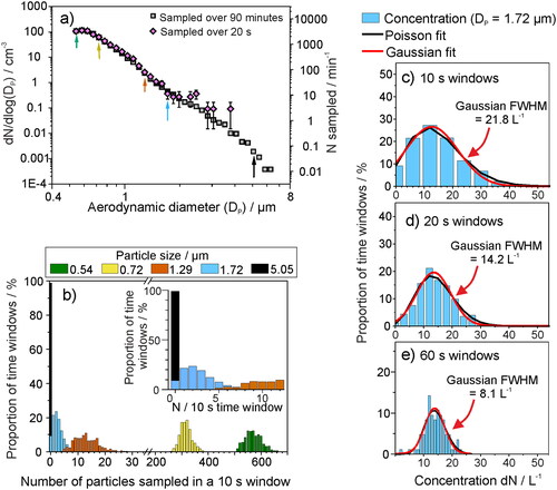
The likelihood of detecting a particle within any single 10 s time window is reported in Figure 5b for five particle sizes, taken from the 90-min sampled data in Figure 5a. The probability function, f(x; λ), of sampled counts in a time window x can be modeled as a Poisson distribution, with a rate λ (Ramachandran and Cooper 2011):(2) $$f\left(x;\mathrm{\lambda }\right)=\frac{{\mathrm{\lambda }}^x\mathrm{ }{e}^{-\mathrm{\lambda }}}{x!}$$(2)

The Poisson function can be well represented by a Normal approximation if the arrival (detection) rate is suffieintly high:(3) $$f\left(x\right)=\frac{A}{\sigma \mathrm{ }\sqrt{\frac{\pi }{2}}}{e}^{\left[{-2\left(\frac{x-x_c}{\sigma }\right)}^2\right]}$$(3) where x_c is the mean of the distribution, A is the amplitude and σ is the standard deviation.

The histograms for the smaller particle sizes (0.54 μm, green; 0.72 μm, yellow; and 1.29 μm, orange) show a form well represented by a normal distribution, demonstrating that an arbitrary 10 s sampling window would provide an accurate mean concentration for these particle sizes. By contrast, 1.72 μm (blue) and 5.05 μm (black) particles are detected with Poisson distributions that cannot be well represented by a Normal distribution. Therefore, reported concentrations for these short sampling windows are limited by the arrival statistics of particles at the detector. Increasing the sampling window improves the reliability of a reported mean (reducing the effect of shot-noise). For 1.72 μm particles, the concentration observed over a sampling window period transitions to a normal function as the sampling window is increased from 10 s, to 20 s, to 60 s (Figure 5c–e). The range of measured concentrations (i.e., full width at half maximum of the resulting Gaussian distribution) narrows from 21.8 L⁻¹ for a 10 s sampling window to 8.1 L⁻¹ for a 60 s sampling window, improving quantification of the large particle concentration. Moreover, at a 60 s sampling window, the mean concentration from the Poisson fit (i.e., λ in Equation (2)(2) $$f\left(x;\mathrm{\lambda }\right)=\frac{{\mathrm{\lambda }}^x\mathrm{ }{e}^{-\mathrm{\lambda }}}{x!}$$(2) ) converges with that of the Gaussian fit (x_c in Equation (3)(3) $$f\left(x\right)=\frac{A}{\sigma \mathrm{ }\sqrt{\frac{\pi }{2}}}{e}^{\left[{-2\left(\frac{x-x_c}{\sigma }\right)}^2\right]}$$(3) ) (Figure 5e) and with the mean concentration for such a particle size across the entire 90 min dataset (14.1 L⁻¹). Therefore, for this particular experiment, an integration time of 60 s is required to quantify accurately the number concentration of 1.72 μm diameter particles.

The concentration of particles within the 5.05 μm bin are >200× lower (Figure 5a) than those in the 1.72 μm size bin, suggesting that a sampling period on the order of hours would be necessary to shift away from an arrival statistics limited measurement and obtain an accurate mean concentration. The concentration of 5 μm particles in room air (dN/dlog(D_p) = 0.00192 cm⁻³, N = 0.06 particles min⁻¹) is similar to that of 8 μm diameter particles generated by a cough (Figure 1b, (Johnson et al. 2011)). Thus, sampling over long timescales (hours to days) is required to gain a reliable mean concentration for the largest respiratory aerosol particles. Otherwise, shot-noise will dominate the arrival statistics, leading to large uncertainty in the mean concentration. The purpose of this example is to emphasize the importance of long sampling windows to reliably obtain accurate size distributions, particularly for larger particles that are low in abundance but carry significant mass. Obviously, in some cases (e.g., coughing, AGPs) peaks of aerosol generation may be short lived and thus cannot be sampled for long periods of time, so comparisons of aerosol size distributions generated at low concentration should be cautiously interpreted.

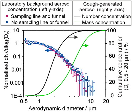
Using sampling instrumentation with higher sampling flow rates and broader bins in the size classification can reduce the time required to sample aerosol accurately and precisely. However, high sample flow rates involve increased challenges associated with inertial impaction and transmission losses within sampling lines due to increases in Stokes number. This is demonstrated in Figure 6 where the background aerosol concentration in a laboratory was sampled by an APS in 30 min intervals over 7 h, either directly by the APS (blue circles) or sampled through 130 cm of conductive silicone tubing and a plastic sampling funnel (pink diamonds). The loss of sampled particles by impaction or diffusion within the tubing/funnel becomes increasingly significant for particle sizes greater than ∼ 4 μm. While challenging to quantify, larger particles may be significant in driving disease transmission if the quantity of pathogen (dose) scales with delivered mass. Figure 6 also reports the cumulative aerosol concentration, in terms of both number (black line) and mass concentration (green line) for a size distribution of aerosol between 0.5 and 20 μm generated by a cough (Johnson et al. 2011). Where the cumulative fraction of aerosol up to 8 micron in diameter makes up 99.7% of number concentration, it only makes up ∼ 85% of the mass concentration. Poor quantification of the concentration of large respiratory particles could therefore lead to large uncertainties in the mass concentration and infection risk.

Figure 6. The size distribution of aerosol sampled by an APS in a chemistry laboratory (background concentration ∼ 20 cm⁻³), normalized with respect to the concentration for D_p = 1 µm, sampled over 30 min periods over a time of ∼7 h, compared with the sampled aerosol through 130 cm of conductive silicone tubing and a sampling funnel (datapoints, left axis). Lines show the cumulative fraction of aerosol generated by a cough (data from Johnson et al. 2011), reported in terms of number and mass concentration fraction.

3.4. Evaporation and transport dynamics of exhaled jets and implications for sampling positioning

Choosing the ideal sampling setup requires consideration of the respiratory aerosol jet dynamics, both in terms of dispersion and evaporation. Respiratory aerosol plumes are generated within a very high (close to 100%) relative humidity (RH) environment, within a warm, moist jet of varying speed according to the type of exhalation. In cold environments, exhaled droplets can initially undergo growth due to the air becoming supersaturated, which is why breath can be visible in cold weather (Ng et al. 2021). However, for an indoor environment with ambient temperature and RH, water will rapidly evaporate from the exhaled particles, reducing their size and altering their transport properties. For larger droplets (>20 μm) the competition among evaporation, sedimentation and momentum has been explored in detail to model the trajectories of respiratory particles (Walker et al. 2021; Xie et al. 2007). By contrast, aerosol particles <20 μm are expected to follow the path of the buoyant jet rather than follow a ballistic trajectory (Bourouiba 2020; Prather et al. 2020). Thus, understanding the trajectory of a respiratory jet helps to determine where best to sample aerosol.

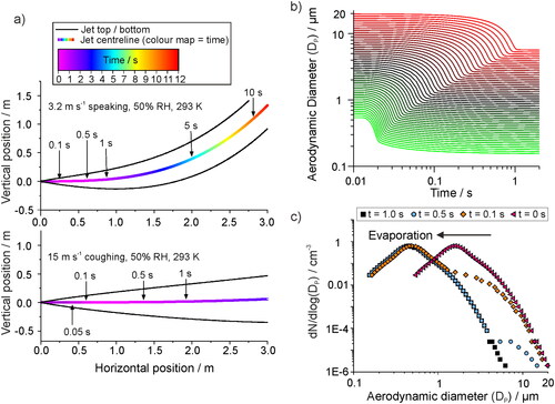
Upon exit from the respiratory tract, the jet will disperse in 3 directions. In general, single particle counting instrumentation should be used to monitor the plume of aerosol as close to the source as possible in order to measure the source strength and minimize effects of dispersion and dilution. However, it may be necessary to sample a distance away from the source to account for logistical constraints (e.g., clinician movement or participant comfort). We model the jet position as a function of time using the model described in Walker et al., based on the treatment of buoyant jets by Liu et al. (Walker et al. 2021; Liu et al. 2017). Whilst the emission rate will be highly subject-dependent, we show an example trajectory of a jet formed by speech (initial jet velocity 3.2 m s⁻¹) and a cough (15 m s⁻¹) in Figure 7a (top and bottom, respectively) with typical indoor environmental conditions of 50% RH and 293 K. The respiratory jet (and the generated aerosol) follow a steady upwards trajectory. Jets with a faster initial velocity are largely unperturbed by the environmental conditions, thus, travel close to horizontal for over 3 m (Figure 7a). In both cases, the jet spreads out after exiting the respiratory tract. When sampling at some distance from the source, the sampling setup (e.g., a funnel) should be constructed such that it spans a large portion of the cross-sectional area of the plume in order to ensure detection of generated aerosol. The 3-dimensional dispersion of aerosol will reduce the sampled concentrations of respiratory aerosol if sampled at a distance from the source, and this will affect the ability to measure all types of exhalation but may be less important for coughs as the respiratory jet starts at a much higher concentration to begin with.

Figure 7. (a) The trajectory of a generated respiratory jet, indicating the path that aerosol droplets of respirable size (<20 µm diameter) would follow, for example flow rates to represent speech (top, 3.2 m s⁻¹) and a cough (bottom, 15 m s⁻¹) in an environment of 50% RH and 293 K. Positive vertical motion is in the upwards direction. (b) The simulated evaporation profiles of saliva droplets from size ranging from 0.5 – 20 µm, in conditions of 293 K and 50% RH. The hygroscopic properties of saliva are considered in the simulation. (c) The size distribution of aerosol particles generated by a cough at the source, as reported by an APS by Johnson et al., and the same plume of aerosol followed by 0.1, 0.5, and 1.0 s transit time.

Evaporation can significantly alter the aerosol size distribution and so must be considered when developing a sampling setup. In the study of Johnson et al., subjects breathed or coughed into an Expiratory Droplet Investigation System (EDIS) where a particle sizer sampled the aerosol a fixed distance away from the participant. The sampled size distribution was assumed to be equilibrated to ambient RH, and a correction factor was introduced to account for the evaporation process and estimate the emitted (high RH) size distribution (Johnson et al. 2011; Morawska et al. 2009). Sampling respiratory emissions directly (<10 cm distance) into a collection funnel can produce a steady state of concentration in the funnel, depending upon the relative flow rate of the exhalation vs the sampling rate, (see Figure 5). Therefore, it can be assumed that the aerosol plume in the funnel is not diluted by the room air. It follows that the respiratory jet of high RH vapor may only be marginally diluted in such a funnel, and that limited evaporation and size changes can occur prior to detection so no such correction is required (Gregson, Watson, et al. 2021; Wilson et al. 2021).

To explore the effects of evaporation on sampling, we simulate the evaporation rate within a plume of aerosol droplets containing artificial saliva at 293 K and 50% RH using the model of Walker et al. (Figure 7b). The hygroscopicity of artificial saliva and surrogate deep lung fluid are similar to each other and are less hygroscopic than NaCl (Walker et al. 2021), which is often used as a proxy for respiratory fluid. These surrogate respiratory fluids do not contain solid cellular material, and so will not fully reflect the complexity of real respiratory droplets. Figure 7b shows simulated evaporation profiles for 0.5–20 μm diameter particles, and Figure 7c shows how evaporation would affect the measured distribution of saliva droplets produced by a cough when measured at specific time points after generation. Sub-micron particles take <0.1 s to equilibrate to ambient RH, which decreases the particle size by less than one third of the initial diameter. Larger particles take longer to evaporate, with 20 μm particles equilibrating to a diameter of 6.24 μm in ∼ 1 s, significantly altering the shape of the size distribution.

These simulations demonstrate that the aerosol plume is best sampled with minimum evaporation and mixing with the surrounding environment (i.e., direct sampling at the source, Case 1 in Figure 4) or after complete evaporation and equilibration has occurred (e.g., as performed by Johnson et al.). In the former, the intensive property of size-dependent aerosol number concentration can be reliably reported. In the latter, the dilution and dispersion of the exhaled jet as well as shifts in particle size must be considered to ensure the accurate concentrations are reported.

3.5. Aerosol source attribution

Many single particle counting instruments are unable to unambiguously discriminate among different particle types (composition and shape). While some sizing instruments use fluorescence techniques to distinguish ‘bioaerosol’ from ‘non biological aerosol’, often the only information retrieved about a plume of sampled aerosol is the concentration and size distribution. Correctly attributing an observed aerosol peak to respiratory origin (and thus carrying an infection risk) is a crucial challenge that requires high time resolution measurements (e.g., 1 s) and comparison of the measured size distributions to those known for respiratory aerosol.

Accurate record keeping of events “timestamped” during a measurement are critical, for instance recording the moment a subject breathes into the sampling funnel or when key processes occur during a clinical procedure. Such practice allows the aerosol generated by the human subject to be correctly identified and distinguished from background and allows aerosol not generated by the subject to be confidently identified as non-respiratory. Some studies report an increased mean concentration during a procedure compared to that during a “background” sampling window, without any time-resolved data to investigate the source of the increased aerosol (Sagami et al. 2021). Whilst such studies are useful in indicating clinical procedures of interest for follow-up studies, taken alone they could be misleading, as the sources of aerosol could be non-respiratory (Doggett, Chow, and Mubareka 2020). During a real clinical procedure, non-respiratory aerosol generation can be frequent. For example, movement near the sampling funnel may resuspend dust, and many materials can themselves generate aerosol. Figure 8a shows aerosol peaks generated in clinical settings when various materials are moved and agitated near the inlet of an OPS in a laminar flow operating theater (0 cm⁻³ background in the 0.3–10 μm size range). Notable peaks include the aerosol generated by green gauze, sterile gauze, and throat pack, which all have peak number concentrations similar to those generated from respiratory activities and could potentially be misassigned as having a respiratory origin unless activities are carefully recorded and timestamped.

Figure 8. (a) The aerosol particle concentration detected by an OPS in a laminar flow operating theater when various different clinical materials are moved past the OPS inlet: I. Rustling green gauze, II. Rustling theater hat, III. Opening non-sterile gauze, IV. Opening sterile gauze, V. Unwrapping tracheal tube, VI. Opening throat pack, VII. Rustling fluid resistant face mask, VIII. Rubbing theater scrubs. (b) The size distribution of particles detected when a throat pack is opened near to the OPS inlet, compared to the aerosol sampled during a voluntary cough (Brown et al. 2020) normalized with respect to the particle size bin of largest concentration. Data are plotted from (Shrimpton, Gregson, Brown, et al. 2021b).

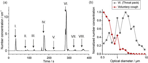
Aerosol size distributions also are valuable to identify aerosol sources. For example, the size distribution of particles generated by the throat pack in Figure 8 forms a lognormal distribution with the peak centered at 2 μm (Figure 8b), different to the size distribution generated by a cough (Brown et al. 2020), which also shows a lognormal distribution but with a peak that is submicron in particle diameter. To accurately assess transmission risk, the aerosol sources must be clearly identified.

3.6. Accounting for intersubject variability in aerosol generation from a range of human subjects

The aerosol generated by a group of subjects typically shows large intersubject variability, forming a log-normal distribution. In other words, there exist minority of “superemitters” who generate much greater quantitities of aerosol than others (Asadi et al. 2019). To accout for this, aerosol generated from the respiratory tract should be sampled from groups of as many subjects as logistically possible. As an example, mean aerosol mass concentrations and standard deviations sampled from a cohort of 25 professional singers are indicative for breathing (0.157 μg m⁻³ with 0.682 SD), speaking at a volume of 70-80 dB (0.312 μg m⁻³ with 0.387 SD) and singing at 70-80 dB (1.004 μg m⁻³ with 0.380 SD), from our previous work (Gregson, Watson, et al. 2021). Based on the means and standard deviations of these activities, to resolve a factor of 2.5 difference in aerosol concentration from different activities, a cohort size of 16 or 21 would be required for a statistical power of 0.8 or 0.9, respectively. In addition, comparisons between the aerosol sampled during different activities (e.g., a cough vs a clinical procedure) can be reported with greater statistical power in fewer subjects if the subject’s own coughs or breathing are used as a reference (Gregson, Shrimpton, et al. 2021).

When reporting an average concentration or size distribution of aerosol generated by a cohort of subjects, the lognormal variability should be considered in the data analysis. For example, instead of reporting a mean concentration in linear space, the mean of logarithmically transformed (Gregson, Watson, et al. 2021; Asadi et al. 2019) or square-root transformed (Johnson et al. 2011) data can be reported for sampled concentrations and size distributions, to account for the large intersubject variability and existence of outliers.

4. Summary and conclusions

Respiratory aerosols are polydisperse, temporally and spatially variable, highly dynamic, and are generated in low concentrations. Consequently, sampling these aerosols is challenging. Accurate measurements are necessary for assessing pathways for respiratory disease transmission and ultimately to guide policy decisions. Moreover, models that predict respiratory aerosol dispersion require robust measurements for inputs and for informed interpretation of results.

This article highlights key considerations for sampling respiratory aerosol. The choice of aerosol instrumentation and environment are crucial. Our recommendations for an ideal measurement are to:

• Use sampling instrumentation that provides size-resolved concentrations across a wide size range with high temporal resolution.

• Ensure there is an extremely low (near zero) background aerosol concentration to confidently identify respiratory aerosol concentrations relative to other potential sources.

• Take an average generated aerosol concentration over a long acquisition time. While respiratory aerosol is often generated in transient events, where possible the exhalation process should be repeated and sampled over long times to accurately record the concentration, particularly for the large particles where very few particles are generated. Care should be taken in drawing definitive comparisons between size distributions in size ranges where the number concentration is very low.

• Consider the relative flow rates of the source and the sampling instrument in order to understand whether to report results as an absolute particle emission rate or as a concentration.

• Sample as close to the source as possible. Respiratory aerosols are embedded within a jet that will expand with distance from the source. Care must be taken in the sampling setup to ensure as large a cross-section of the jet as possible is intercepted.

• Consider how ambient RH may alter aerosol size due to evaporation over timescales that may be of similar magnitude to the measurement period.

• Account for the lognormal variability in aerosol generated among different people by aiming for cohorts of ∼25 people.

This contribution focuses largely on sampling particles <20 μm diameter, where instrumental approaches are already robust and commercially available. By contrast, few methods have been reported to characterize quantitatively droplets 20 – >100 μm, which are likely to be important vectors for the transmission of many diseases. Future efforts are also needed to focus on developing similarly robust approaches to routinely measure the number concentrations and size distributions of these larger droplets.

Acknowledgments

The authors acknowledge the AERATOR group, which consists of (in alphabetical order): Arnold, D; Brown, J; Bzdek, B; Davidson, A; Dodd, J; Gormley M; Gregson, F; Hamilton, F; Maskell, N; Murray, J; Keller, J; Pickering, A.E; Reid, J; Sheikh, S; Shrimpton, A. We acknowledge the Working Group for The Investigation of ParticulatE Respiratory Matter Release During perFormance and Exercise to infOrm Guidance in the SARS-CoV-2 PandeMic (PERFORM 2) for useful discussions.

Disclosure statement

The authors declare no competing interests.

Data availability

Data are available in the BioStudies database (https://www.ebi.ac.uk/biostudies/) under accession number S-BSST718.

Additional information

Funding

The AERATOR study was funded by an NIHR-UKRI rapid rolling grant (COV0333). H.E.S. and J.A. are supported by the PERFORM 2 study, funded by UKRI-EPSRC (EP/V050516/1). B.R.B. is supported by the Natural Environment Research Council (NE/P018459/1). The views and opinions expressed by authors in this publication are those of the authors and do not necessarily reflect those of the NHS, the NIHR, UKRI, or the Department of Health.

References

- Almstrand, A. C., B. Bake, E. Ljungström, P. Larsson, A. Bredberg, E. Mirgorodskaya, and A. C. Olin. 2010. Effect of airway opening on production of exhaled particles. J. Appl. Physiol. 108:584–8. doi: 10.1152/japplphysiol.00873.2009.
- Alsved, M., A. Matamis, R. Bohlin, M. Richter, P. E. Bengtsson, C. J. Fraenkel, P. Medstrand, and J. Löndahl. 2020. Exhaled respiratory particles during singing and talking. Aerosol Sci. Technol. 54:1245–8. doi: 10.1080/02786826.2020.1812502.
- Asadi, S., A. S. Wexler, C. D. Cappa, S. Barreda, N. M. Bouvier, and W. D. Ristenpart. 2019. Aerosol emission and superemission during human speech increase with voice loudness. Sci. Rep. 9:1–10. doi: 10.1038/s41598-019-38808-z.
- Bar-On, Y. M., A. Flamholz, R. Phillips, and R. Milo. 2020. SARS-CoV-2 (COVID-19) by the numbers. Elife 9:e57309. doi: 10.7554/eLife.57309.
- Bourouiba, L. 2020. Turbulent gas clouds and respiratory pathogen emissions potential implications for reducing transmission of COVID-19. JAMA Insights 323:1837–8. doi: 10.1001/jama.2020.4756.
- Bourouiba, L. 2021. The fluid dynamics of disease transmission. Annu. Rev. Fluid Mech. 53:473–508. doi: 10.1146/annurev-fluid-060220-113712.
- Bourouiba, L., E. Dehandschoewercker, and J. W. M. Bush. 2014. Violent expiratory events: On coughing and sneezing. J. Fluid Mech. 745:537–63. doi: 10.1017/jfm.2014.88.
- Brown, J., F. K. A. Gregson, A. Shrimpton, T. M. Cook, B. R. Bzdek, J. P. Reid, and A. E. Pickering. 2020. A quantitative evaluation of aerosol generation during tracheal intubation and extubation. Anaesthesia 76:174–181. doi: 10.1111/anae.15292.
- Carroll, R. G. 2007. Elsevier’s integrated physiology, 1st ed. Philadelphia, PA: Elsevier, 99–115.
- Charlotte, N. 2020. High rate of SARS-CoV-2 transmission due to choir practice in France at the beginning of the COVID-19 pandemic. J. Voice. doi: 10.1016/j.jvoice.2020.11.029.
- Damit, B., C. Y. Wu, and M. D. Cheng. 2014. On the validity of the Poisson assumption in sampling nanometer-sized aerosols. Aerosol Sci. Technol. 48:562–70. doi: 10.1080/02786826.2014.899682.
- Doggett, N., C.-W. Chow, and S. Mubareka. 2020. Characterization of experimental and clinical bioaerosol generation during potential aerosol-generating procedures. Chest 158:2467–73. doi: 10.1016/j.chest.2020.07.026.
- Gaeckle, N. T., J. Lee, Y. Park, G. Kreykes, M. D. Evans, and C. J. Hogan. 2020. Aerosol generation from the respiratory tract with various modes of oxygen delivery. Am. J. Respir. Crit. Care Med. 202:1115–24. doi: 10.1164/rccm.202006-2309oc.
- Gregson, F. K. A., A. J. Shrimpton, F. W. Hamilton, T. M. Cook, J. P. Reid, A. E. Pickering, D. J. Pournaras, B. R. Bzdek, and J. M. Brown. 2021. Identification of the source events for aerosol generation during oesophago-gastro-duodenoscopy. Gut. doi: 10.1136/gutjnl-2021-324588.
- Gregson, F. K. A., N. A. Watson, C. M. Orton, A. E. Haddrell, L. P. McCarthy, T. J. R. Finnie, N. Gent, G. C. Donaldson, P. L. Shah, J. D. Calder, et al. 2021. Comparing aerosol concentrations and particle size distributions generated by singing, speaking and breathing. Aerosol Sci. Technol. 55:681–91. doi: 10.1080/02786826.2021.1883544.
- Hamilton, F. W., D. Arnold, B. R. Bzdek, J. W. Dodd, Aerator Group, J. P. Reid, and N. Maskell. 2021a. Aerosol generating procedures: are they of relevance for transmission of SARS-CoV-2? Lancet Respir. Med. 2600:1–2. doi: 10.1016/S2213-2600(21)00216-2.
- Hamilton, F. W., F. K. A. Gregson, D. T. Arnold, S. Sheikh, K. Ward, J. Brown, E. Moran, C. White, A. Morley, B. R. Bzdek, et al. 2021b. Aerosol emission from the respiratory tract: an analysis of relative risks from oxygen delivery systems. medRxiv 1–19. doi: 10.1101/2021.01.29.21250552.
- Herfst, S., E. J. A. Schrauwen, M. Linster, S. Chutinimitkul, E. de Wit, V. J. Munster, E. M. Sorrell, T. M. Bestebroer, D. F. Burke, D. J. Smith, et al. 2012. Airborne transmission of influenza A/H5N1 virus between ferrets. Science 336:1534–41. doi: 10.1126/science.1213362.
- Holmgren, H., E. Ljungström, A.-C. Almstrand, B. Bake, and A.-C. Olin. 2010. Size distribution of exhaled particles in the range from 0.01 to 2.0μm. J. Aerosol Sci. 41:439–46. doi: 10.1016/j.jaerosci.2010.02.011.
- Johnson, G. R., L. Morawska, Z. D. Ristovski, M. Hargreaves, K. Mengersen, C. Y. H. Chao, M. P. Wan, Y. Li, X. Xie, D. Katoshevski, et al. 2011. Modality of human expired aerosol size distributions. J. Aerosol Sci. 42:839–51. doi: 10.1016/j.jaerosci.2011.07.009.
- Larsen, M. L. 2007. Spatial distributions of aerosol particles: Investigation of the poisson assumption. J. Aerosol Sci. 38:807–22. doi: 10.1016/j.jaerosci.2007.06.007.
- Lednicky, J. A., M. Lauzard, Z. H. Fan, A. Jutla, T. B. Tilly, M. Gangwar, M. Usmani, S. N. Shankar, K. Mohamed, A. Eiguren-Fernandez, et al. 2020. Viable SARS-CoV-2 in the air of a hospital room with COVID-19 patients. Int. J. Infect. Dis. 100:476–82. doi: 10.1016/j.ijid.2020.09.025.
- Li, Y., X. Huang, I. T. S. Yu, T. W. Wong, and H. Qian. 2005. Role of air distribution in SARS transmission during the largest nosocomial outbreak in Hong Kong. Indoor Air 15:83–95. doi: 10.1111/j.1600-0668.2004.00317.x.
- Liu, Y., Ning, Z. Chen, Y., M. Guo, Y.Liu, N. K. Gali, L. Sun, Y. Duan, J. Cai, D. Westerdahl, X. Liu, K Xu, et al. 2020. Aerodynamic analysis of SARS-CoV-2 in two Wuhan hospitals. Nature 582:557–60. doi:10.1038/s41586-020-2271-3.
- Liu, L., J. Wei, Y. Li, and A. Ooi. 2017. Evaporation and dispersion of respiratory droplets from coughing. Indoor Air. 27 (1):179–90. doi:10.1111/ina.12297.
- Llandro, H., J. R. Allison, C. C. Currie, D. C. Edwards, C. Bowes, J. Durham, N. Jakubovics, N. Rostami, and R. Holliday. 2021. Evaluating splatter and settled aerosol during orthodontic debonding: implications for the COVID-19 pandemic. Br. Dent. J. doi: 10.1038/s41415-020-2503-9.
- McCarthy, L. P., C. M. Orton, N. A. Watson, F. K. A. Gregson, A. E. Haddrell, W. J. Browne, J. D. Calder, D. Costello, J. P. Reid, P. L. Shah, et al. 2021. Aerosol and droplet generation from performing with woodwind and brass instruments. Aerosol Sci. Technol. 55:1277–87. doi: 10.1080/02786826.2021.1947470.
- McGhee, C. N. J., S. Dean, S. E. N. Freundlich, A. Gokul, M. Ziaei, D. V. Patel, R. L. Niederer, and H. V. Danesh-Meyer. 2020. Microdroplet and spatter contamination during phacoemulsification cataract surgery in the era of COVID-19. Clin. Experiment. Ophthalmol. 48:1168–74. doi: 10.1111/ceo.13861.
- Mellies, U., and C. Goebel. 2014. Optimum insufflation capacity and peak cough flow in neuromuscular disorders. Annals Ats. 11:1560–8. doi: 10.1513/AnnalsATS.201406-264OC.
- Morawska, L., G. R. Johnson, Z. D. Ristovski, M. Hargreaves, K. Mengersen, S. Corbett, C. Y. H. Chao, Y. Li, and D. Katoshevski. 2009. Size distribution and sites of origin of droplets expelled from the human respiratory tract during expiratory activities. J. Aerosol Sci. 40:256–69. doi: 10.1016/j.jaerosci.2008.11.002.
- Mürbe, D., M. Fleischer, J. Lange, H. Rotheudt, and M. Kriegel. 2020. Aerosol emission is increased in professional singingof classical music. Sci. Rep. 11:14861. doi: 10.1038/s41598-021-93281-x.
- Newsom, R. B., A. Amara, A. Hicks, M. Quint, C. Pattison, B. R. Bzdek, J. Burridge, C. Krawczyk, J. Dinsmore, and J. Conway. 2021. Comparison of droplet spread in standard and laminar flow operating theatres: SPRAY study group. J. Hosp. Infect. 110:194–200. doi: 10.1016/j.jhin.2021.01.026.
- Ng, C. S., K. L. Chong, R. Yang, M. Li, R. Verzicco, and D. Lohse. 2021. Growth of respiratory droplets in cold and humid air. Phys. Rev. Fluids 6:054303. doi: 10.1103/PhysRevFluids.6.054303.
- Pöhlker, M. L., O. O. Krüger, J.-D. Förster, W. Elbert, J. Fröhlich-Nowoisky, U. Pöschl, C. Pöhlker, G. Bagheri, E. Bodenschatz, J. A. Huffman, et al. 2021. Respiratory aerosols and droplets in the transmission of infectious diseases. arXiv 1–50, arXiv: 2103.01188v4
- Prather, K. A., L. C. Marr, R. T. Schooley, M. A. McDiarmid, M. E. Wilson, and D. K. Milton. 2020. Airborne transmission of SARS-CoV-2. Science 370:303–4. doi: 10.1126/science.abf0521.
- Ramachandran, G., and D. W. Cooper. 2011. Size distribution data analysis and presentation. In Aerosol Measurement: Principles, Techniques, and Applications, eds. P. Kulkarni, P.A. Baron, K. Willeke, 488, Hoboken, New Jersey: John Wiley & Sons.
- Ratnesar-Shumate, S., K. Bohannon, G. Williams, B. Holland, M. Krause, B. Green, D. Freeburger, and P. Dabisch. 2021. Comparison of the performance of aerosol sampling devices for measuring infectious SARS-CoV-2 aerosols. Aerosol Sci. Technol. 55:975–86 doi: 10.1080/02786826.2021.1910137.
- Sagami, R., H. Nishikiori, T. Sato, H. Tsuji, M. Ono, K. Togo, K. Fukuda, K. Okamoto, R. Ogawa, K. Mizukami, et al. 2021. Aerosols produced by upper gastrointestinal endoscopy: A quantitative evaluation. Am. J. Gastroenterol. 116:202–5. doi:10.14309/ajg.0000000000000983.
- Shrimpton, A., F. K. A. Gregson, J. M. Brown, T. M. Cook, B. R. Bzdek, F. Hamilton, J. P. Reid, and A. E. Pickering. 2021. A quantitative evaluation of aerosol generation during supraglottic airway insertion and removal. Anaesthesia. 76:16–18 doi: 10.1111/anae.15345.
- Shrimpton, A., F. K. A. Gregson, T. M. Cook, J. Brown, B. R. Bzdek, J. P. Reid, and A. E. Pickering. 2021. A quantitative evaluation of aerosol generation during tracheal intubation and extubation: a reply. Anaesthesia 76:16–29. doi: 10.1111/anae.15345.
- Stadnytskyi, V., C. E. Bax, A. Bax, and P. Anfinrud. 2020. The airborne lifetime of small speech droplets and their potential importance in SARS-CoV-2 transmission. Proc. Natl. Acad. Sci. U. S. A. 117:11875–877. doi: 10.1073/pnas.2006874117.
- Tellier, R., Y. Li, B. J. Cowling, and J. W. Tang. 2019. Recognition of aerosol transmission of infectious agents: A commentary. BMC Infect. Dis. 19:101. doi: 10.1186/s12879-019-3707-y
- Tran, K., K. Cimon, M. Severn, C. L. Pessoa-Silva, and J. Conly. 2011. Aerosol-generating procedures and risk of transmission of acute respiratory infections: a systematic review [Internet]. Ottawa: Canadian Agency for Drugs and Technologies in Health. Accessed March 2021. Available from: http://www.cadth.ca/media/pdf/M0023__Aerosol_Generating_Procedures_e.pdf/.
- Vette, A. F., A. W. Rea, G. Evans, V. R. Highsmith, L. Sheldon, P. A. Lawless, and C. E. Rodes. 2001. characterization of indoor-outdoor aerosol concentration relationships during the fresno PM exposure studies. Aerosol Sci. Technol. 34:118–26. doi: 10.1080/02786820117903.
- Volckens, J., and T. M. Peters. 2005. Counting and particle transmission efficiency of the aerodynamic particle sizer. J. Aerosol Sci. 36:1400–8. doi: 10.1016/j.jaerosci.2005.03.009.
- Vuorinen, V., M. Aarnio, M. Alava, V. Alopaeus, N. Atanasova, M. Auvinen, N. Balasubramanian, H. Bordbar, P. Erästö, R. Grande, et al. 2020. Modelling aerosol transport and virus exposure with numerical simulations in relation to SARS-CoV-2 transmission by inhalation indoors. Saf. Sci. 130:104866. doi:10.1016/j.ssci.2020.104866.
- Walker, J. S., J. Archer, F. K. A. Gregson, S. E. S. Michel, B. R. Bzdek, and J. P. Reid. 2021. Accurate representations of the microphysical processes occurring during the transport of exhaled aerosols and droplets. ACS Cent. Sci. 7:200–9. doi: 10.1021/acscentsci.0c01522.
- Wilson, N. M., G. B. Marks, A. Eckhardt, A. M. Clarke, F. P. Young, F. L. Garden, W. Stewart, T. M. Cook, and E. R. Tovey. 2021. The effect of respiratory activity, non-invasive respiratory support and facemasks on aerosol generation and its relevance to COVID-19. Anaesthesia 76:1465–74. doi: 10.1111/anae.15475.
- Xie, X.,. Y. Li, A. T. Y. Chwang, P. L. Ho, and W. H. Seto. 2007. How far droplets can move in indoor environments – revisiting the Wells evaporation–falling curve. Indoor Air. 17:211–25. doi: 10.1111/j.1600-0668.2006.00469.x.
- Yan, J., M. Grantham, J. Pantelic, P. J. B. De Mesquita, B. Albert, F. Liu, S. Ehrman, and D. K. Milton. 2018. Infectious virus in exhaled breath of symptomatic seasonal influenza cases from a college community. Proc. Natl. Acad. Sci. U. S. A. 115:1081–6. doi: 10.1073/pnas.1716561115.