The use of acoustic streaming in Sub-micron particle sorting

Abstract

The lack of personal particulate matter (PM) monitoring technique hinders the knowledge of the negative health impacts caused by inhaling PM. Acoustophoresis has a potential to produce miniature particle sorters that can be carried inside human’s breath zone. Micron particles can be manipulated by Acoustic Radiation Force (ARF), but sub-micron particles can hardly be directed due to Acoustic Streaming Effect (ASE). The purpose of this study is to examine the feasibility of sorting sub-micron particles using ASE. In this study, a 2 D numerical model is used to simulate the movement of sub-micron particles, ranging from 0.1 µm to 0.9 µm in diameter with 0.1 µm step size, suspended in a microchannel. Since tiny particles circulate according to the streaming pattern, which depends on the geometry of the container, the effect of the microchannel’s cross-sectional shape on particle movement is investigated, from rectangular to non-rectangular. Results found that sub-micron particles are characterized as either ARF-dominant or ASE-dominant. ARF-dominant particles stop at the pressure node and sidewalls, while ASE-dominant particles are trapped by the streaming flow inside a certain area defined by the particle size. Larger ASE-dominant particles move in a narrower region close to the sidewalls; smaller particles occupy a wider area. Since ASE-dominant particles can be directed outside the settling location of ARF-dominated particles, separating them can reach 98.9% purity in a non-rectangular microchannel. Most importantly, separating ASE-dominant particles of different sizes is shown possible using a triangular microchannel. The findings imply that ASE can be the mechanism for sub-micron particle sorting.

Copyright © 2021 American Association for Aerosol Research

EDITOR:

• Jonathan P. Reid

1. Introduction

Nowadays, people raise concern over the health impacts of particulate matter (PM) (Shao et al. 2021; Othman and Latif 2021; Chen, Jia, and Han 2021). Not only may the inhalation of ultrafine particles (UFPs) cause cardiovascular and pulmonary diseases (Jaques and Kim 2000; Sioutas, Delfino, and Singh 2005), but aerosols can also act as virus carriers (Bontempi 2020; Nor et al. 2021; Comunian et al. 2020). Despite the increasing PM-related health concerns, the exact mechanisms causing health problems and the particle size range that is particularly harmful to human health remain unclear (Reich, Fuentes, and Burke 2008). The lack of information on personal exposure level is one of the reasons that lead to the knowledge gap (Sioutas, Delfino, and Singh 2005).

Conventional nanoparticle measurement techniques are bulky devices that are intended for stationary field testing, not for measuring personal exposure level. Studies showed that there are differences between personal PM exposure level and the background PM level found in stationary measurements (Pietroiusti and Magrini 2014; Koponen, Koivisto, and Jensen 2015; Jørgensen, Buhagen, and Føreland 2016). The actual exposure level is highly related to the activities of the person (Ferro, Kopperud, and Hildemann 2004; Buonanno, Stabile, and Morawska 2014; Ryan et al. 2015), which may draw more PM into the breathing zone. Estimating the personal exposure level by summing a limited number of examined areas that a person has visited is very inaccurate. However, carrying the bulky devices in the breathing zone is impractical. Furthermore, nanoparticle sizers often require radioactive sources, which is not safe to place them near occupants. Therefore, it is essential to develop small portable measurement devices to monitor the personal PM level as Individuals move within microenvironments. Recently, Lee et al. (2019) developed a small UFPs size analyzer using electrostatics techniques. Our study aims to further reduce the size of the PM measurement devices by using Acoustophoresis on lap-on-a-chip devices.

Microfluidics has introduced numerous benefits to aerosol science, not only shrinking the device size scale, but also such as reducing the sampling volume and reagent, having a high flexibility in device design, reducing the experiment scale, and being cost effective. Metcalf, Narayan, and Dutcher (2018) summarized the microfluidic concepts that have been employed in aerosol studies and discussed extensively the potential applications. Furthermore, Liu, Ng, and Lu (2021) reported that microfluidic techniques can overcome some challenges associated with PM toxicity studies. Integrating microfluidics into aerosol science can possibly lower the current limitations. For our purpose, aerosol sorting, a compact lap-on-a-chip device is an excellent alternative to the traditional bulky devices. On a lap-on-a-chip device, different mechanisms can be employed to manipulate particle movement, such as dielectrophoretic, magnetic, optical, and acoustic techniques (Sajeesh and Sen 2014). In this study, we apply the concept of acoustics to aerosol sorting with a microfluidic platform.

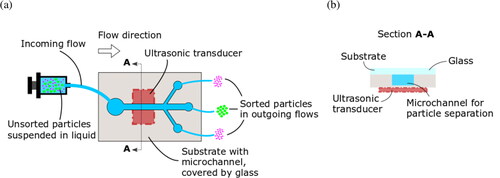
Application of acoustophoresis to cell and particle separation in microchannel draws increasing attention in many disciplines in the past decades due to its high precision and minimum damage to the matters of interest (Salafi, Zeming, and Zhang 2016; Wu et al. 2019; Sajeesh and Sen 2014). The standard setup includes a microchannel and an ultrasound actuator that generates an acoustic field inside the microchannel (Zhang et al. 2020; Ding et al. 2012; Gupta and Bit 2019). A mixture of unsorted particles suspended in liquid flows from the inlet of the microchannel to the acoustic field region, where the fluid suspensions is directed by the acoustic radiation forces (ARF) to the pressure nodes or antinodes (Figure 1a). Since larger particles would experience a stronger ARF, they would move faster to the pressure nodes or antinodes. Dividing the flow at specific locations can therefore separate particles of different sizes. Petersson et al. (2007) employed this phenomenon extensively and developed a free flow acoustophoresis method that combines laminar flow with axial ARF to demonstrate the possibility of sorting polystyrene particles with sizes ranging from 2 µm to 10 µm simultaneously. More separation technologies have been developed in the last decades, for which Lenshof and Laurell (2010) summarized the important features.

Figure 1. (a) Schematic diagram of an ordinary experimental setup for studying the acoustophoretic particle sorting inside a microchannel; (b) side view of the experimental setup showing the cross-sectional shape of the microchannel.

However, there exists a lower size limit for ARF-driven devices. As the particle size goes down, the significance of the acoustic streaming effect (ASE) grows and becomes a hurdle since small particles tend to circulate according to the streaming vortices (Yuen, Fu, and Chao 2017). They become inseparable from the particles settled on the pressure node. Muller et al. (2012) developed a numerical model that considers both ARF and ASE to illustrate the transition in particle motion when the particle size decreases. It is found that the movement of larger particles is dominated solely by ARF. When the particle size drops to the first threshold, the influence of ASE starts to take effect, and the strength increases as the particle size decrease. Finally, when the particle size reaches the second threshold, its motion is no longer affected by ARF but solely driven by ASE. The first and second thresholds depend mainly on the frequency of ultrasound excitation, the geometry of the microchannel, and the viscosity of the liquid medium that fills the microchannel. Since the ASE has been considered as an obstacle to particle manipulation, its suppression becomes a common goal to improve the effectiveness of particle separation (Karlsen et al. 2018; Bach and Bruus 2020).

To break through the development boundary, researchers started to utilize the ASE to manipulate particle movement. Although the ASE obstructs particles from moving toward the pressure node, it drives particles to flow in a streaming current. Devendran, Gralinski, and Neild (2014) demonstrated the application of ASE on particle separation in an open microchannel. The 3 µm particles are driven by the ASE and follow the streaming vortex to the air-liquid interface in their device. Then, the particles are collected from the free surface at high purity. The use of ASE provides a new approach to acoustophoretic particle separation. Instead of trapping the particles located on the pressure node, particles swirling in the streaming flow can also be collected. This idea shows the possibility of using ASE to capture submicron PM from ambient air.

Since tiny particles tend to circulate according to the streaming pattern, modifying the streaming pattern is a potential method to control the particle movement. Studies showed that the streaming pattern changes with the geometry confining it (Yuen, Fu, and Chao 2016; Yuen et al. 2014). For a rectangular microchannel, the streaming pattern usually appears as four streaming vortices in the bulk (two rows by two columns) (Wiklund, Green, and Ohlin 2012). These streaming vortices are called Rayleigh streaming, which are driven by a counter-rotating vortex inside the boundary layer. The vortices inside the boundary layer are the Schlichting streaming, which are formed by the velocity gradient inside the boundary layer caused by the viscous loss. As the streaming pattern is coupled to the microchannel’s cross-sectional shapes, in this article, we will study the effect of a series of cross-sectional shapes, from rectangle, to trapezoidal and triangle on particle movement numerically. A numerical model for calculating acoustic streaming and acoustophoretic motion of particles will be developed and validated by experimental data found in the literature. The objective of this study is to examine the feasibility of sorting sub-micron particles using ASE in non-rectangular microchannels.

2. Methodology

In this numerical study, we considered a bulk acoustic wave device at resonance mode, in which a transducer attached to the bottom of the microchannel generates acoustic waves that propagate in the vertical direction. The other walls act as reflectors, resulting in a standing wave that allows particle manipulation. To model this phenomenon, we first defined the simulation domain, the cross-sectional area of the microchannel within the acoustic actuation region, which can be viewed by cutting section A-A in Figure 1a. We considered only the confined fluid (Figure 1b). Regarding the study on the influence of the cross-sectional shape, five geometries were included. Figure 2 shows the schematic diagrams of the five cases with the coordinate systems used for the study. They all have a bottom wall of 160 µm and a height of 100 µm. The alternation was done by decreasing the sidewalls inclination from 90° (rectangle) to 51.35° (triangle). As we changed the geometry of the microchannel, the resonance frequency alters accordingly. Hence, the excitation frequencies in Case 1 to Case 5 are 7.5 MHz, 7.45 MHz, 7.38 MHz, 7.45 MHz, and 8.16 MHz, respectively.

Figure 2. Simulation domains of the five studied cases with the coordinate system employed in this numerical study.

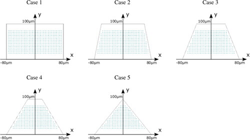
To begin with, we employed the governing equations of fluid motion to estimate the acoustic field and streaming inside the domain. Then, we distributed particles in the domain to study the particle migration. The motion of 9 different particle sizes was analyzed, ranging from 0.1 µm to 0.9 µm in diameter with a step size of 0.1 µm. To illustrate the difference between micron and submicron particles’ motion, the movement of 3.8 µm particles was also included. Particles of different sizes were disturbed in the same way. Their initial positions are shown in Figure 2. Since the cross-sectional area reduces from Case 1 to Case 5, the number of particles released to the microchannel decreases to maintain uniform density, which is 510, 438, 372, 306, and 204, respectively.

For this study, the fluid medium was defined as water at 25 °C, while the suspended particles were polystyrene spheres. The material parameters were taken from Spigarelli et al. (2020) and listed in Table 1. The acoustic contributions to the system were considered small perturbations, and thus the standard perturbation theory for the thermoacoustic field was employed. The zeroth-order represents the fluid state before the acoustic contributions. We solved the first-order variables to obtain the acoustic pressure field. The results were used to compute the second-order variables, which represent the streaming flow. Finally, the particle motion was calculated by Lagrangian particle tracking. For this study, COMSOL Multiphysics 5.5 was employed as the numerical solver to understand the underlying mechanisms that govern the acoustophoretic motion of suspended particles.

Table 1. The material parameters used for water at 25 °C and polystyrene Spigarelli et al. (2020).

Water at 25 °C (T0)
Density	${\rho }_0$	998 [kg/m^3]
Speed of sound	$c_0$	1497 [m/s]
Dynamic viscosity	$\mu$	0.890 [mPa s]
Bulk viscosity	${\mu }_B$	2.485 [mPa s]
Thermal conductivity	$k$	0.6065 [W/mK]
Specific heat capacity	$C_p$	4181 [J/(kg K]]
Specific heat capacity ratio	$\gamma$	1.011
Isobaric thermal expansion coefficient	${\alpha }_p$	0.2573 [1/mK]
Isentropic compressibility^1	$\kappa$	448 [1/TPa]
Isothermal compressibility^2	${\beta }_T$	453 [1/TPa]
Polystyrene particles
Density	${\rho }_p$	1050 [kg/m^3]
Speed of sound	$c_p$	2350 [m/s]
Compressibility	${\sigma }_p$	249 [1/TPa]
Poisson’s ratio	${\kappa }_p$	0.35

¹ Calculated from $\kappa =1/\left({\rho }_0{c}_0^2\right).$

² Calculated from ${\beta }_T=\gamma \kappa .$

3. Governing equations

The theory of acoustics in a fluid can be described by combining the continuity equation (Equation (1)(1) $${\partial }_t\rho +\nabla ·\left(\rho \mathit{v}\right)=0,$$(1) ), the Navier-Stokes equation for compressible Newtonian liquid (Equation (2)(2) $$\rho \left[{\partial }_t\mathit{v}+\left(\mathit{v}·\nabla \right)\mathit{v}\right]=\nabla ·\left\{-p\mathit{I}+\mu \left[\nabla \mathit{v}+{\left(\nabla \mathit{v}\right)}^T\right]-\left(\frac{2}{3}\mu -{\mu }_B\right)\left(\nabla ·\mathit{v}\right)\mathit{I}\right\},$$(2) ), the heat transfer equation (Equation (3)(3) $$\rho T\left({\partial }_{t}s+\mathit{v}·\nabla s\right)=\nabla ·\left(k\nabla T\right),$$(3) ), and the thermodynamic relations (Equation (4)(4) $$\rho =\rho \left(p,T\right),$$(4) ). As a fluid dynamics problem, a complete description of the acoustic field can be obtained by solving the velocity field and any two of the thermodynamic variables of the fluid. (1) $${\partial }_t\rho +\nabla ·\left(\rho \mathit{v}\right)=0,$$(1) (2) $$\rho \left[{\partial }_t\mathit{v}+\left(\mathit{v}·\nabla \right)\mathit{v}\right]=\nabla ·\left\{-p\mathit{I}+\mu \left[\nabla \mathit{v}+{\left(\nabla \mathit{v}\right)}^T\right]-\left(\frac{2}{3}\mu -{\mu }_B\right)\left(\nabla ·\mathit{v}\right)\mathit{I}\right\},$$(2) (3) $$\rho T\left({\partial }_{t}s+\mathit{v}·\nabla s\right)=\nabla ·\left(k\nabla T\right),$$(3) (4) $$\rho =\rho \left(p,T\right),$$(4) where $\rho$ is the density, $\mathit{v}$ is the velocity, $p$ is the pressure, $\mu$ is the dynamic viscosity, ${\mu }_B$ is the bulk viscosity when the compressibility is important (Dukhin and Goetz 2009; Graves and Argrow 1999), $T$ is the temperature, $s$ is the entropy, and $k$ is the thermal conductivity of the fluid.

As mentioned earlier, the system of equations was solved by the perturbation method. The perturbation series can be written as: (5a) $$\rho ={\rho }_0+{\rho }_1+{\rho }_2,$$(5a) (5b) $$p=p_0+p_1+p_2,$$(5b) (5c) $$T=T_0+T_1+T_2,$$(5c) (5d) $$\mathit{v}={\mathit{v}}_0+{\mathit{v}}_1+{\mathit{v}}_{2,}$$(5d)

Before the acoustic contribution, we considered a quiescent fluid (${\mathit{v}}_0=0$) in thermodynamic equilibrium with a constant density (${\rho }_0$), constant pressure ($p_0$) and constant temperature ($T_0$). Solving the first-order and second-order quantities gave the acoustic field and steady acoustic streaming flow. The acoustic actuation was modeled as boundary conditions. A harmonic oscillation was applied to the actuated wall (Equation (6a)(6a) $${\mathit{v}}_{\mathit{actuated}}=\left[\begin{array}{c}{v}_{\mathit{actuated},x}\\ v_{\mathit{actuated},y}\end{array}\right]=\left[\begin{array}{c}0\\ \omega l_0{e}^{-i\omega t}\end{array}\right],$$(6a) ). The other microchannel’s walls were assumed rigid and acoustically hard, thereby reflecting incoming waves (Equation (6b)(6b) $${\mathit{v}}_{\mathit{wall}}=0,$$(6b) ). (6a) $${\mathit{v}}_{\mathit{actuated}}=\left[\begin{array}{c}{v}_{\mathit{actuated},x}\\ v_{\mathit{actuated},y}\end{array}\right]=\left[\begin{array}{c}0\\ \omega l_0{e}^{-i\omega t}\end{array}\right],$$(6a) (6b) $${\mathit{v}}_{\mathit{wall}}=0,$$(6b) (6c) $$T_{\mathit{wal}}=T_0,$$(6c) where ${\mathit{v}}_{\mathit{actuated}}$ is the velocity of the actuated wall (bottom wall), $\omega$ is the angular frequency of the harmonic oscillation, $l_0$ is the displacement of the bottom wall, ${\mathit{v}}_{\mathit{wall}}$ is the velocity of other microchannel’s walls. Under the resonance mode, supported by experiments, a typical value for $l_0$ is 0.1 nm (Dual and Schwarz 2012; Barnkob et al. 2010).

For the first-order fields, we assumed a harmonic time dependence $e^{-i\omega t}$ from the actuation wall. Inserting Equation (5)(5a) $$\rho ={\rho }_0+{\rho }_1+{\rho }_2,$$(5a) into Equations (1)(1) $${\partial }_t\rho +\nabla ·\left(\rho \mathit{v}\right)=0,$$(1) to (4)(4) $$\rho =\rho \left(p,T\right),$$(4) , and collecting terms up to first-order, we had (7) $$i\omega {\rho }_1+\nabla ·\left({\rho }_0{\mathit{v}}_1\right)=0,$$(7) (8) $$i\omega {\rho }_0{\mathit{v}}_1=\nabla ·\left\{-p_1\mathit{I}+\mu \left[\nabla {\mathit{v}}_1+{\left(\nabla {\mathit{v}}_1\right)}^T\right]-\left(\frac{2}{3}\mu -{\mu }_B\right)\left(\nabla ·{\mathit{v}}_1\right)\mathit{I}\right\},$$(8) (9) $${\rho }_0{C}_p\left(i\omega T_1+{\mathit{v}}_1·\nabla T_0\right)-{\alpha }_p{T}_0\left(i\omega p_1+{\mathit{v}}_1·\nabla p_0\right)=\nabla ·\left(k\nabla T_1\right),$$(9) (10) $${\rho }_1={\rho }_0\left({\beta }_T{p}_1-{\alpha }_p{T}_1\right),$$(10)

To obtain Equations (9)(9) $${\rho }_0{C}_p\left(i\omega T_1+{\mathit{v}}_1·\nabla T_0\right)-{\alpha }_p{T}_0\left(i\omega p_1+{\mathit{v}}_1·\nabla p_0\right)=\nabla ·\left(k\nabla T_1\right),$$(9) and (10)(10) $${\rho }_1={\rho }_0\left({\beta }_T{p}_1-{\alpha }_p{T}_1\right),$$(10) , we considered the thermodynamic relation $ds=\frac{C_p}{T}dT-\frac{{\alpha }_p}{\rho }dp$ and ${\partial }_t\rho =\rho {\beta }_T{\partial }_{t}p-\rho {\alpha }_p{\partial }_{t}T,$ respectively, in which $C_p$ is the specific heat capacity of the fluid at constant pressure, ${\alpha }_p$ is the fluid isobaric thermal expansion coefficient, and ${\beta }_T$ is the fluid isothermal compressibility.

For the second-order fields, we considered the steady-state of the streaming flow and assume the flow is incompressible. We did not treat the periodic behavior due to the acoustic field but only calculate the time-averaged motion. Inserting the entire perturbation series (Equations 5a(5a) $$\rho ={\rho }_0+{\rho }_1+{\rho }_2,$$(5a) to 5d(5d) $$\mathit{v}={\mathit{v}}_0+{\mathit{v}}_1+{\mathit{v}}_{2,}$$(5d) ) into Equations 1(1) $${\partial }_t\rho +\nabla ·\left(\rho \mathit{v}\right)=0,$$(1) to 2(2) $$\rho \left[{\partial }_t\mathit{v}+\left(\mathit{v}·\nabla \right)\mathit{v}\right]=\nabla ·\left\{-p\mathit{I}+\mu \left[\nabla \mathit{v}+{\left(\nabla \mathit{v}\right)}^T\right]-\left(\frac{2}{3}\mu -{\mu }_B\right)\left(\nabla ·\mathit{v}\right)\mathit{I}\right\},$$(2) , substituting Equations 7(7) $$i\omega {\rho }_1+\nabla ·\left({\rho }_0{\mathit{v}}_1\right)=0,$$(7) to 10(10) $${\rho }_1={\rho }_0\left({\beta }_T{p}_1-{\alpha }_p{T}_1\right),$$(10) , and then taking average of the quantities, we had (11) $${\rho }_0\nabla ·〈{\mathit{v}}_2〉=-\nabla ·〈{\rho }_1{\mathit{v}}_1〉,$$(11) (12) $$0=-〈\nabla p_2〉+\nabla ·\left[\mu \left(\nabla 〈{\mathit{v}}_2〉+{\left(\nabla 〈{\mathit{v}}_2〉\right)}^T\right)\right]-〈{\rho }_1\left({\partial }_t{\mathit{v}}_1\right)〉-{\rho }_0〈\left({\mathit{v}}_1·\nabla \right){\mathit{v}}_1〉,$$(12) where $〈\mathit{q}〉=\frac{1}{t}{\int }_0^{t}dt\mathit{q}\left(t\right)$ is the time-averaged quantities over an entire oscillational period.

For the motion of the suspended particles, the time-averaged acoustophoretic motion would be calculated. There are other studies that consider the time harmonic motion of the suspensions. The time harmonic motion is significant when the excitation frequency is below the upper limit set by the particle relaxation time (Dain et al. 1995). In our study, the excitation frequency is well above that upper limit. Thus, the time harmonic effect on the particle can be accurately neglected. Regarding the forces exerted on the particles, as the buoyancy force balances the gravitational forces, they are negligible to other acoustic forces (Glynne-Jones and Hill 2013). Thus, the particle motion was calculated by considering the Stokes drag force and the ARF (Equation (13)(13) $$m_p{\mathit{a}}_p=F^{\mathit{drag}}+F^{\mathit{rad}},$$(13) ). (13) $$m_p{\mathit{a}}_p=F^{\mathit{drag}}+F^{\mathit{rad}},$$(13) where $m_p$ is the mass of the suspended particle, ${\mathit{a}}_p$ is the particle acceleration, $F^{\mathit{drag}}$ is the Stokes drag force, and $F^{\mathit{rad}}$ is the ARF.

For a suspended particle with a radius a moving at velocity v_p, the Stokes drag force is given by Equation (14)(14) $$F^{\mathit{drag}}=6\pi \mu a\left(〈{\mathit{v}}_2〉-{\mathit{v}}_p\right),$$(14) (Stokes 2009), (14) $$F^{\mathit{drag}}=6\pi \mu a\left(〈{\mathit{v}}_2〉-{\mathit{v}}_p\right),$$(14)

We considered the time-averaged ARF as developed by Settnes and Bruus (2012) (Equation (15)(15) $$F^{\mathit{rad}}=-\pi a^3\left[\frac{2\kappa }{3}Re\left[f_1{p}_1\nabla p_1\right]-{\rho }_{0}Re\left[f_2{v}_1·\nabla v_1\right]\right],$$(15) ). The coefficients $f_1$ and $f_2$ can be obtained from Settnes and Bruus (2012) and $\kappa$ is the fluid isentropic compressibility, $\kappa =1/\left({\rho }_0{c}_0^2\right).$ (15) $$F^{\mathit{rad}}=-\pi a^3\left[\frac{2\kappa }{3}Re\left[f_1{p}_1\nabla p_1\right]-{\rho }_{0}Re\left[f_2{v}_1·\nabla v_1\right]\right],$$(15)

4. Grid analysis and model validation

4.1. Grid analysis

The mesh was generated by COMSOL Multiphysics 5.5 using triangular elements. Considering that the thermal and viscous losses occur near the boundaries, the element size d decreases gradually to resolve the thermal and viscous boundary layers. To do so, we considered the thickness of the boundary layers in the mesh generation: (16) $${\delta }_T=\sqrt{\frac{2\kappa }{\omega {\rho }_0{C}_p}},$$(16) (17) $${\delta }_V=\sqrt{\frac{2\nu }{\omega }},$$(17) where ${\delta }_T$ and ${\delta }_V$ are the thicknesses of the thermal and viscous boundary layers, respectively. 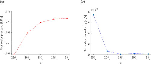Near the boundaries, the element size $d$ is set smaller than ${\delta }_T$ and ${\delta }_V.$ In the fluid bulk, $d$ is set to be multiples of ${\delta }_V$ to reduce the computational time. In the grid analysis, we performed a series of simulations with an increasing level of refinement ($d=25{\delta }_V,20{\delta }_V,15{\delta }_V,10{\delta }_V,5{\delta }_V$). For results comparison, we presented the results obtained from a point at the center of the microchannel ([x,y] = [80 µm,50 µm]) in Figure 3. Figure 3a shows the first-order pressure (p₁), and Figure 3b shows the second-order velocity (${\mathit{v}}_2$). The grid analysis results indicate both the first- and second-order results coverage. The differences in the results between 10${\delta }_V$ and 5${\delta }_V$ under the graphs are 0.005% and 0.4%, respectively. Further refining the mesh would not bring a significant impact on the results. Therefore, we concluded that $d=10{\delta }_V$ can achieve adequate accuracy, and so it was employed in this study.

Figure 3. The grid analysis results: (a) the first-order pressure ($p_1$), and (b) the second-order velocity (${\mathit{v}}_2$).

4.2. Model validation

In this section, we computed two study cases found in the literature to validate our model. First, the numerical results obtained by Muller et al. (2012) were used for the validation of the acoustic fields. Then, the experimental results obtained by Barnkob et al. (2010) were used for the validation of the particle movement.

Muller et al. (2012) studied a microchannel with a width 380μm and a height 160μm under a harmonic excitation frequency 1.97 MHz on the sidewalls. We reconstructed the test case. A comparison of the results is shown in Table 2. Notably, we compared the first-order horizontal velocity component obtained near the bottom wall (Figure 4a). Figure 4a indicates that the generated mesh can resolve the boundary layers. For the ASE part of the model, Figure 4b shows the time-averaged second-order velocity obtained from our model, which is comparable, in terms of both vector plot and magnitude, to the results from Muller et al. (2012). Since the differences are small, we could claim that the presented model has adequate accuracy.

Figure 4. The model validation results: (a) first-order horizontal velocity component obtained at $y=0\mathrm{}to\mathrm{}2\mathrm{\mu }m;$ (b) time-averaged second-order velocity (the color plot shows the magnitude, and the arrows indicate the direction); (c) particle displacement changes with time.

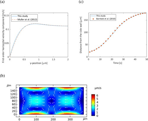
Table 2. A comparison between the results obtained in this study and the study conducted by Muller et al. (2012).

	Results obtained from this study	Results obtained from Muller et al. (20012)
First-order pressure amplitude	0.243133 MPa	0.24 MPa
First-order temperature amplitude	5.561421mK	5mK
Maximum first-order horizontal velocity component	0.161489m/s	0.162m/s

As our focus is on the particle movement, we would like to have experimental evidence to support our results. Barnkob et al. (2010) built a microfluidic resonator with a silicon/glass microchannel and a piezo actuator. The geometry of the microchannel is 377μm (width) by 157μm (height). Under an excitation frequency of 1.994 MHz, the movement of the 5.16μm polystyrene microbead is recorded by a CCD camera. We inputted the test conditions into our numerical model and found that the particle takes around 5 s to reach the pressure node. Figure 4c shows how the particle displacement changes with time. The accuracy of the presented model in particle movement was also confirmed since our results agree well with the experimental results. It should be noted that, the movement of 5.16μm polystyrene microbead is dominated by ARF. Thus, only the movement of large particle is experimentally validated. For the small particles, since the ARF effect on them becomes insignificant, they would have the same velocity as the fluid particles that they are in contact with (Stokes 2009). In other words, they should follow the streaming flow.

5. Results

5.1. Acoustic pressure field

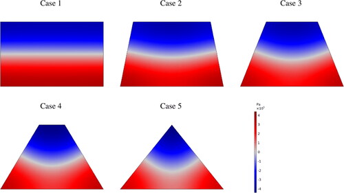
The ultrasonic actuation generates an acoustic field inside the microchannel. Due to the reflection of the walls, a standing wave is formed in all cases. The cross-sectional shape of the microchannel slightly affects the magnitude of the acoustic pressure field. The pressure amplitude increases on the top wall but decreases on the bottom wall from Case 1 to Case 5 (Table 3), changing the field strength from symmetric between the top and bottom halves in the rectangular case to asymmetric in the non-rectangular cases. The variation increases with the wall inclination, indicating that the geometry has the potential to concentrate the acoustic field. The narrower top wall generates a stronger pressure field. However, it comes with a weaker field on the bottom half.

Table 3. Acoustic pressure amplitude on the top and bottom walls of the microchannel.

Case	1	2	3	4	5
Excitation Frequency	7.50 MHz	7.45 MHz	7.38 MHz	7.45 MHz	8.16 MHz
Acoustic pressure amplitude on the top wall	0.361 MPa	0.378 MPa	0.381 MPa	0.434 MPa	0.440 MPa
Acoustic pressure amplitude on the bottom wall	0.361 MPa	0.361 MPa	0.337 MPa	0.331 MPa	0.302 MPa

Since the studied geometries are symmetric about the y-axis, a left-right symmetrical pressure field distribution is generated in all cases (Figure 5). In Case 1, the wave travels vertically and is reflected solely by the upper wall. The pressure node appears as a straight line located at $y=h/2.$ In other cases, the side walls are inclined, thereby taking part in the wave reflection. Thus, the pressure node is not a straight line, but appears as a curve bent toward the bottom wall. The curvature increases from Case 2 to Case 5.

Figure 5. Acoustic pressure field in the five studied cases.

5.2. Acoustic streaming

The geometry of the microchannel has altered the acoustic streaming velocity and pattern accordingly. In Figure 6, the arrows show the direction of the streaming flow. The size of the arrows represents the magnitude of the streaming velocity in the logarithmic scale. In all cases, the streaming pattern is also left-right symmetric. Four vortices are generated in the bulk, two above the pressure node line and two below, which are counter-rotating compared to the neighboring vortices. They are Rayleigh’s streaming. Due to the different length-scale, Schlichting streaming cannot be shown in Figure 6. The region of Schlichting streaming is very narrow near the walls. In Figure 6, the highest streaming velocity is found near the sidewalls. It may be explained by the fact that Rayleigh’s streaming is induced by the strong streaming vortices formed inside the viscous layer (Schlichting streaming), and the streaming velocity is the largest at the point where the streaming flow is initiated. The flow becomes weaker as it moves away from the sidewalls.

Figure 6. Acoustic streaming pattern in the five studied cases.

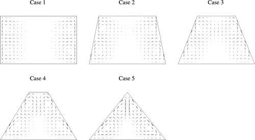
In Case 1, the four vortices are identical in size and magnitude. They occupy the sides of the microchannel, leaving the center lightly affected by the ASE. As the sidewall inclination increases from Case 2 to Case 5, the center of the vortices moves toward the vertical centerline. Hence, the fraction of the computational domain affected by the ASE increases. In Case 2, the streaming vortices are like those found in Case 1, but the top vortices are placed closer. In Case 3, the top vortices collide, resulting in a substantial streaming flow along the top centerline. The center of the lower half of the microchannel remains unaffected. As the wall inclination further increases, the top vortices become smaller than the bottom vortices in Case 4 and Case 5. At the same time, the steaming flow seems equally strong across the cross-section except for the lower center region.

5.3. Acoustophoretic motion of sub-micron particles

In this section, the resulting movement of sub-micron particles caused by ARF and ASE will be discussed. Figure 7 shows the end location of 3.8 µm, 0.9 µm, 0.4 µm, 0.1 µm particles, while their movement can be found in Figure 1S in the supplementary information. As expected, the 3.8 µm particles are driven solely by ARF moving straight to the pressure node and become stationary, while submicron particles tend to settle in the streaming flow. Notably, this behavior is size-dependent, thereby allowing the separation of submicron particles. In addition to the particle size, the cross-sectional shape also plays a role in the acoustophoretic motion.

Figure 7. The end location of 3.8 µm, 0.9 µm, 0.4 µm, and 0.1 µm particles.

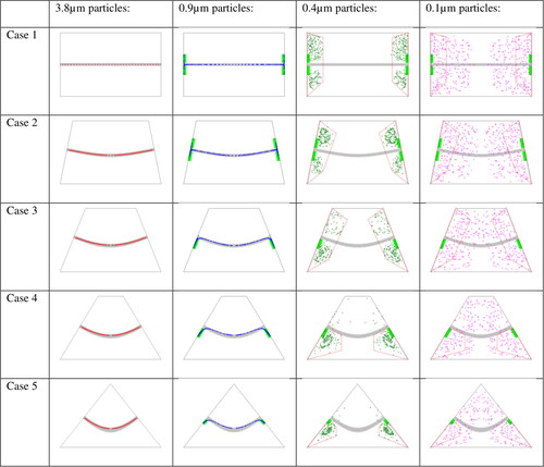
The motion of submicron particles can be divided into two categories: ARF-dominant and ASE-dominant. In our model, the threshold is set at 0.8 µm, which is independent of the microchannel geometry. Particles larger than that are considered as ARF-dominant since they come to rest after some time, while particles smaller than that are ASE-dominant. The ASE-dominant particles do not stop even after a significant long time but circulate in the streaming vortices. They seem to be trapped by ASE inside a certain region. However, the settling time is not comparable to the ARF-driven motion. Sub-micron particles require a longer time to settle. Table 4 shows the settling time of the 3.8 µm (t3.8), 0.9 µm (t0.9), 0.4 µm (t0.4), 0.1 µm (t0.1) particles in the studies cases.

Table 4. The settling time of the 3.8 µm, 0.9 µm, 0.4 µm, and 0.1 µm particles in Case 1 to Case 5.

	Case 1	Case 2	Case 3	Case 4	Case 5
t3.8	0.03s	0.035s	0.05s	0.06s	0.07s
t0.9	0.4s	0.4s	0.7s	1s	1.2s
t0.4	10s	7s	7s	6s	6s
t0.1	10s	7s	6s	6s	6s

5.3.1. Movement of ARF-driven particles (3.8 µm particles)

The 3.8 µm particles settle on the pressure node line quickly. The cross-sectional shape varies the settling time (t_3.8). In the rectangular case, the particle movement involves only the vertical motion since the pressure gradient along the x-direction is negligible. In contrast, the movement also includes a horizontal component in the non-rectangular cases. The horizontal displacement increases from Case 2 to Case 5, which is related to the increased curvature of the pressure field. Particles above the pressure node line move faster than the ones below, reflecting the stronger pressure field generated on the top. Although the pressure amplitude increases from Case 1 to Case 5, the overall pressure field weakens, resulting in a decreasing vertical displacement. The gray region in Figure 7 is defined as the settling location of 3.8 µm particles, which will be used to discuss the particle separation performance in the next section.

5.3.2. Movement of ARF-dominant sub-micron particles (0.9 µm particles)

The movement of 0.9 µm particles depends on the particles’ location. Here, we divided the computational domains into two sections: (1) the center and (2) near sidewalls. Particles in the center are driven to the pressure node and stay there. They follow the path of 3.8 µm particles, but they are more than ten times slower. The particle velocity decreases from Case 1 to Case 5. Particles near sidewalls move in the direction of the streaming flow. They are found coming to the sidewalls. At t_0.9, all particles are settled, either on the pressure node line or at the sidewalls. Since the settling location is beyond the gray region, here we defined a green region to confine the 0.9 µm particles that fall outside the gray region.

5.3.3. Movement of ASE-dominant sub-micron particles (0.4 µm and 0.1 µm particles)

Although the ASE-dominant particles do not stop, they eventually settle inside some regions. These regions confining the particles become stable over time, whose final shape depends on the particle size. Bigger particles flow into a smaller region close to the sidewalls where the streaming flow is initiated, and smaller particles circulate the streaming vortices in a wider area (Figure 7).

Shortly after t_0.9, most 0.4 µm particles are already trapped inside the end location area by the streaming flow, but some fall inside the gray area, where ASE is weak, and need a significantly longer time to get out, especially Case 1. A possible reason is that, in Case 1, a larger fraction of the cross-sectional area is weakly affected by ASE. At t_0.4, the particles move inside a certain area that is slightly off the gray area. In Case 1 and Case 2, the eddies above the pressure node are a little bigger than the ones below; in Case 3, the eddies below the pressure node become larger; in Case 4 and Case 5, most particles are trapped below the pressure node.

In contrast, fewer 0.1 µm particles arrive the gray region. They remain inside the area that is affected by ASE, for which the cross-sectional shape takes up an important role. In Case 1, a large fraction of the domain is with shallow streaming velocity; particles released there need more time to enter the streaming vortices. From Case 2 to Case 5, the significance of the ASE increases, therefore the required time for ASE to trap particles reduces. The results indicate that the wall inclination may enhance ASE-driven particle movement. In all cases, four almost equally dense eddies are formed. The end location of the particles overlaps the pressure node slightly.

5.4. Novel approach of sub-micron particle sorting by ASE

Conventional acoustophoretic particle sorting devices are ARF-driven, which draw particles to the pressure node and then separate them from the rest of the mixture. Due to ASE, sub-micron particles can hardly settle on the pressure nodes. Hence, sorting sub-micron particles has never been achieved, nor has their movement been treated. But now, our results indicate that, by utilizing ASE and designing the cross-section shape of the microchannel properly, it is possible to sort sub-micron particles by acoustophoresis.

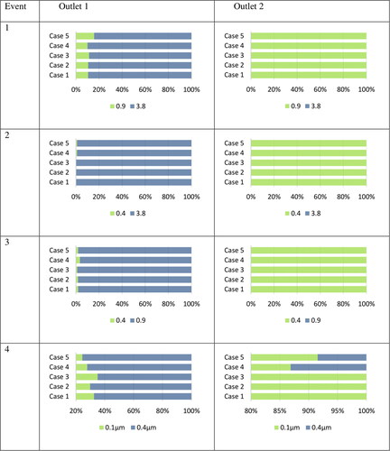
To investigate the particle-sorting performance, we consider the following four events: 1) separating ARF-dominant sub-micron particles and ARF-driven particles (0.9 µm and 3.8 µm); 2) separating ASE-dominant sub-micron particles and ARF-driven particles (0.4 µm and 3.8 µm); 3) separating ASE-dominant and ARF-dominant sub-micron particles (0.4 µm and 0.9 µm); and 4) separating ASE-dominant sub-micron particles (0.1 µm and 0.4 µm). The separation strategy is to split the flow into two Outlets: Outlet 1 and Outlet 2. How the flow is divided depends on the events that will be described below.

5.4.1. Separation of ARF-dominant sub-micron particles and ARF-driven particles (0.9 µm and 3.8 µm)

In the separation of 0.9 µm and 3.8 µm particles (Event 1), Outlet 1 would be the gray region defined in Figure 7; Outlet 2 would be the remaining area (outside the gray region). Since both 0.9 µm and 3.8 µm particles move toward the gray region, the separation should occur at t_3.8. The later the flow is divided, the more 0.9 µm would fall on the gray region and leave the microchannel with the 3.8 µm particles from Outlet 1. Figure 8 shows the content of the samples collected from Outlet 1 and Outlet 2. In the following, purity is defined as the ratio of the number of target particles to the total number of particles in a sample. The geometry has little impact on the results. Among them, Case 4 performs moderately better. In the collected samples, the purity of 0.9 µm and 3.8 µm particles reaches 100% and 90%, respectively.

Figure 8. Content of the samples collected from Outlet 1 and Outlet 2 in the four events.

5.4.2. Separation of ASE-dominant sub-micron particles and ARF-driven particles (0.4 µm and 3.8 µm)

For this combination (Event 2), Outlet 1 would still be the gray region defined in Figure 8; Outlet 2 would be the remaining area. As ASE would drive 0.4 µm particles away from Outlet 1, the separation should take place after t_0.4, when all 0.4 µm particles are in the streaming flow. The geometry has virtually no impact on the sorting performance. All cases achieve nearly 100% purity on both 0.4 µm and 3.8 µm particles.

5.4.3. Separation of ASE-dominant and ARF-dominant sub-micron particles (0.4 µm and 0.9 µm)

For Event 3, Outlet 1 would be the gray and green regions defined in Figure 9; Outlet 2 would be the remaining area. Again, the separation should take place after t_0.4 since the settling location of 0.9 µm particles is slightly away from the streaming flow. With the contribution of ASE, 0.4 µm and 0.9 µm particles are well separated in all cases. The purities of all collected samples are above 96.5%. Among them, Case 3 is the best, which achieves 100% and 98.9% purity on 0.4 µm and 0.9 µm particles, respectively.

Figure 9. Schematic diagram of the particle sorting system using ASE.

5.4.4. Separation of ASE-dominant sub-micron particles (0.1 µm and 0.4 µm)

To separate 0.1 µm and 0.4 µm particles (Event 4), Outlet 1 would be the area enclosed by the red dash line defined in Figure 7; Outlet 2 would be the remaining area. As presented in the previous section, ASE-dominant sub-micron particles circulate inside a limited space near the walls at the steady state. Thus, the separation should happen after t_0.1 and t_0.4.

In Case 1 to Case 3, the purity of 0.1 µm can reach 100% because the reddish line means to confine all 0.4 µm particles in Outlet 1. However, in Case 4 and Case 5, a few 0.4 µm particles scatter above the pressure node line. Including those 0.4 µm particles in Outlet 1 would lead to an unsuccessful separation since most 0.1 µm particles would also appear in Outlet 1. With the current design, the purities of 0.1 µm particles in Case 4 and Case 5 can maintain over 87%. The purity of 0.4 µm particles is affected by the geometry. In Case 1 and Case 3, the purities are relatively low (below 70%). The most excellent results are found in Case 5, by which the purity of 0.1 µm and 0.4 µm particles are 92.2% and 75.6%, respectively.

5.5. Feasibility of utilizing ASE in sub-micron particle sorting systems

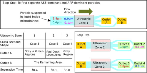
Lastly, we would like to study the feasibility of simultaneously sorting 0.1 µm, 0.4 µm, 0.9 µm, and 3.8 µm particles using ASE. We propose to sort the particles in two steps with three ultrasonic zones (Figure 9). In the first step, ASE-dominant particles are separated from ARF-dominant particles in ultrasonic zone 1. Then, in the second step, ASE-dominant particles are separated in ultrasonic zone 2, while ARF-dominant particles are separated in ultrasonic zone 3. Outlets of the ultrasonic zones and the separation time are indicated in Figure 9. At the end of the system, there are four outlets, Outlet 1 collecting 0.4 µm particles, Outlet 2 collecting 0.1 µm particles, Outlet 3 collecting 3.8 µm particles, and Outlet 4 collecting 0.9 µm particles. Since the purpose of this section is to illustrate the potential of applying ASE in sub-micron particles sorting, we select the optimal cross-sectional shape for the ultrasonic zones. Thus, it would be Case 3 for zone 1, Case 5 for zone 2, and Case 4 for zone 3.

In ultrasonic zone 1, 1.1% of 0.4 µm particles and 4.8% of 0.1 µm particles are lost in the flow of ARF-dominant particles. They appear as the impurity in ultrasonic zone 3 through which 0.9 µm and 3.8 µm particles are collected with purity 88.7% and 95.4%, respectively. Since ultrasonic zone 2 contains solely 0.4 µm and 0.1 µm particles, 0.1 µm and 0.4 µm particles are collected with purity 75.6% and 92.2%, respectively. The results indicate that sorting sub-micron particles by ASE is possible. Further modification on microchannel’s geometry would improve the samples’ purity.

6. Conclusions

For the purpose of developing a miniature PM analyzer, this study has investigated the influence of the microchannel’s cross-sectional shape on the acoustophoretic effect and examined the feasibility of sub-micron particle sorting using ASE with lap-on-a-chip devices. We found that the wall inclination increases the acoustic pressure amplitude but reduces the overall average pressure. The geometry also alters the streaming pattern. For the movement of sub-micron particles, it can be characterized as ARF- and ASE-dominant. Larger particles are ARF-dominant, which concentrate to some region and stop; while smaller particles are ASE-dominant, which continue to circulate inside a certain area defined by the particle size. The bigger ones circulate in a narrower region. These phenomena enable sub-micron particle sorting. With the help of ASE, separating ASE-dominant particles from ARF-dominant particles can reach 100% and 98.9% purity on 0.4 µm and 0.9 µm particles, respectively, in Case 3. Notably, separating ASE-dominant particles of different sizes is shown possible. In Case 5, the purity of 0.1 µm and 0.4 µm particles achieves 92.2% and 75.6%, respectively. It is also possible to separate multi particle sizes simultaneously in a two-step separation process. ARF- and ASE-dominant particles are first separated by ASE, then the ARF- dominant particles and ASE-dominant particles are separated by ARF and ASE, respectively.

The findings reflect the excellent potential of ASE in the development of aerosols sorting systems on microfluidic platforms, whereby the size-scale of aerosol measurement systems can be greatly reduced, and thus aerosol studies can be conducted with a higher flexibility. As being cost-effective, miniature aerosol sorters can be produced at a large volume and placed precisely at the locations of interest, thereby enhancing the study outcomes of aerosol science. However, there remains a separation latency issue about our PM sorting approach. Further studies on the effect of the fluid medium may be able to speed up the separation process.

Disclosure statement

No potential conflict of interest was reported by the authors.

Additional information

Funding

This work was supported by Hong Kong Special Administrative Region Government under Collaborative Research Fund (CRF) (project no. C7025-16G) and General Research Fund (GRF) (project no.16206918).

References

- Bach, J. S., and H. Bruus. 2020. Suppression of acoustic streaming in shape-optimized channels. Phys. Rev. Lett. 124 (21):214501.
- Barnkob, R., P. Augustsson, T. Laurell, and H. Bruus. 2010. Measuring the local pressure amplitude in microchannel acoustophoresis. Lab Chip. 10 (5):563–70. doi:10.1039/b920376a.
- Bontempi, E. 2020. First data analysis about possible COVID-19 virus airborne diffusion due to air particulate matter (PM): The case of Lombardy (Italy). Environ. Res. 186:109639. doi:10.1016/j.envres.2020.109639.
- Buonanno, G., L. Stabile, and L. Morawska. 2014. Personal exposure to ultrafine particles: the influence of time-activity patterns. Sci. Total Environ. 468–469 (468):903–7. doi:10.1016/j.scitotenv.2013.09.016.
- Chen, B., P. Jia, and J. Han. 2021. Role of indoor aerosols for COVID-19 viral transmission: a review. Environ. Chem. Lett. 19 (3):1953–70. doi:10.1007/s10311-020-01174-8.
- Comunian, S., D. Dongo, C. Milani, and P. Palestini. 2020. Air pollution and COVID-19: The role of particulate matter in the spread and increase of COVID-19’s morbidity and mortality. IJERPH. 17 (12):4487. doi:10.3390/ijerph17124487.
- Dain, Y., M. Fichman, C. Gutfinger, D. Pnueli, and P. Vainshtein. 1995. Dynamics of suspended particles in a two-dimensional high-frequency sonic field. J. Aerosol Sci. 26 (4):575–594.
- Devendran, C., I. Gralinski, and A. Neild. 2014. Separation of particles using acoustic streaming and radiation forces in an open microfluidic channel. Microfluid. Nanofluid. 17 (5):879–90. doi:10.1007/s10404-014-1380-4.
- Ding, X., S. S. Lin, M. I. Lapsley, S. Li, X. Guo, C. Y. Chan, I. Chiang, L. Wang, J. P. McCoy, and T. J. Huang. 2012. Standing surface acoustic wave (SSAW) based multichannel cell sorting. Lab Chip. 12 (21):4228–31. doi:10.1039/c2lc40751e.
- Dual, J., and T. Schwarz. 2012. Acoustofluidics 3: Continuum mechanics for ultrasonic particle manipulation. Lab Chip. 12 (2):244–52. doi:10.1039/c1lc20837c.
- Dukhin, A. S., and P. J. Goetz. 2009. Bulk viscosity and compressibility measurement using acoustic spectroscopy. J. Chem. Phys. 130 (12):124519.
- Ferro, A., R. Kopperud, and L. Hildemann. 2004. Elevated personal exposure to particulate matter from human activities in a residence. J. Expo. Sci. Environ. Epidemiol. 14 (S1):S34–S40. doi:10.1038/sj.jea.7500356.
- Glynne-Jones, P., and M. Hill. 2013. Acoustofluidics 23: Acoustic manipulation combined with other force fields. Lab Chip. 13 (6):1003–10. doi:10.1039/c3lc41369a.
- Graves, R. E., and B. M. Argrow. 1999. Bulk viscosity: past to present. J. Thermophys. Heat Transf 13 (3):337–42. doi:10.2514/2.6443.
- Gupta, S., and A. Bit. 2019. Acoustophoresis-based biomedical device applications. In Bioelectronics and medical devices, 123–44. Cambridge: Woodhead Publishing.
- Jaques, P. A., and C. S. Kim. 2000. Measurement of total lung deposition of inhaled ultrafine particles in healthy men and women. Inhal. Toxicol. 12 (8):715–31.
- Jørgensen, R. B., M. Buhagen, and S. Føreland. 2016. Personal exposure to ultrafine particles from PVC welding and concrete work during tunnel rehabilitation. Occup. Environ. Med. 73 (7):467–73.
- Karlsen, J. T., W. Qiu, P. Augustsson, and H. Bruus. 2018. Acoustic streaming and its suppression in inhomogeneous Fluids. Phys. Rev. Lett. 120 (5):054501.
- Koponen, I. K., A. J. Koivisto, and K. A. Jensen. 2015. Worker exposure and high time-resolution analyses of process-related submicrometre particle concentrations at mixing stations in two paint factories. Ann. Occup. Hyg. 59 (6):749–63. doi:10.1093/annhyg/mev014.
- Lee, S., H. Kim, H. Kwon, K. Kim, S. Yoo, U. Hong, J. Hwang, and Y. Kim. 2019. MEMS based particle size analyzer using electrostatic measuring techniques. 2019 20th International Conference on Solid-State Sensors, Actuators and Microsystems & Eurosensors XXXIII (TRANSDUCERS & EUROSENSORS XXXIII): 1289–92.
- Lenshof, A., and T. Laurell. 2010. Continuous separation of cells and particles in microfluidic systems. Chem. Soc. Rev. 39 (3):1203–17.
- Liu, F., N. L. Ng, and H. Lu. 2021. Emerging applications of microfluidic techniques for in vitro toxicity studies of atmospheric particulate matter. Aerosol Sci. Technol. 55 (6):623–39. doi:10.1080/02786826.2021.1879373.
- Metcalf, A. R., S. Narayan, and C. S. Dutcher. 2018. A review of microfluidic concepts and applications for atmospheric aerosol science. Aerosol Sci. Technol. 52 (3):310–29. doi:10.1080/02786826.2017.1408952.
- Muller, P. B., R. Barnkob, M. J. H. Jensen, and H. Bruus. 2012. A numerical study of microparticle acoustophoresis driven by acoustic radiation forces and streaming-induced drag forces. Lab Chip. 12 (22):4617–27. doi:10.1039/c2lc40612h.
- Nor, N. S. M., C. W. Yip, N. Ibrahim, M. H. Jaafar, Z. Z. Rashid, N. Mustafa, H. H. A. Hamid, K. Chandru, M. T. Latif, P. E. Saw, et al. 2021. Particulate matter (PM2.5) as a potential SARS-CoV-2 carrier. Sci. Rep. 11 (1):2508.
- Othman, M., and M. T. Latif. 2021. Air pollution impacts from COVID-19 pandemic control strategies in Malaysia. J. Clean Prod. 291:125992. doi:10.1016/j.jclepro.2021.125992.
- Petersson, F., L. Åberg, A. M. Swärd-Nilsson, and T. Laurell. 2007. Free flow acoustophoresis: microfluidic-based mode of particle and cell separation. Anal. Chem. 79 (14):5117–23.
- Pietroiusti, A., and A. Magrini. 2014. Engineered nanoparticles at the workplace: current knowledge about workers’ risk. Occup. Med. 64 (5):319–30. doi:10.1093/occmed/kqu051.
- Reich, B. J., M. Fuentes, and J. Burke. 2008. Analysis of the effects of ultrafine particulate matter while accounting for human exposure. Environmetrics 20 (2):131–46. doi:10.1002/env.915.
- Ryan, P. H., S. Y. Son, C. Wolfe, J. Lockey, C. Brokamp, and G. LeMasters. 2015. A field application of a personal sensor for ultrafine particle exposure in children. Sci. Total Environ. 508:366–73. doi:10.1016/j.scitotenv.2014.11.061.
- Sajeesh, P., and A. K. Sen. 2014. Particle separation and sorting in microfluidic devices: a review. Microfluid. Nanofluid. 17 (1):1–52. doi:10.1007/s10404-013-1291-9.
- Salafi, T., K. K. Zeming, and Y. Zhang. 2016. Advancements in microfluidics for nanoparticle separation. Lab Chip. 17 (1):11–33. doi:10.1039/c6lc01045h.
- Settnes, M., and H. Bruus. 2012. Forces acting on a small particle in an acoustical field in a viscous fluid. Phys. Rev. E. 85 (1):016327. doi:10.1103/PhysRevE.85.016327.
- Shao, L., S. Ge, T. Jones, M. Santosh, L. F. O. Silva, Y. Cao, M. L. S. Oliveira, M. Zhang, and K. BéruBé. 2021. The role of airborne particles and environmental considerations in the transmission of SARS-CoV-2. Geosci. Front 12 (5):101189. doi:10.1016/j.gsf.2021.101189.
- Sioutas, C., R. J. Delfino, and M. Singh. 2005. Exposure assessment for atmospheric ultrafine particles (UFPs) and implications in epidemiologic research. Environ Health Perspect 113 (8):947–55. doi:10.1289/ehp.7939.
- Spigarelli, L., N. S. Vasile, C. F. Pirri, and G. Canavese. 2020. Numerical study of the effect of channel aspect ratio on particle focusing in acoustophoretic devices. Sci. Rep. 10 (1):19447.
- Stokes, G. 2009. On the effect of the internal friction of fluids on the motion of pendulums. In Mathematical and physical papers, 1–10. Cambridge: Cambridge University Press.
- Wiklund, M., R. Green, and M. Ohlin. 2012. Acoustofluidics 14: Applications of acoustic streaming in microfluidic devices. Lab Chip. 12 (14):2438–51. doi:10.1039/c2lc40203c.
- Wu, M., A. Ozcelik, J. Rufo, Z. Wang, R. Fang, and T. Jun Huang. 2019. Acoustofluidic separation of cells and particles. Microsyst. Nanoeng. 5:32. doi:10.1038/s41378-019-0064-3.
- Yuen, W. T., S. C. Fu, and C. Y. Chao. 2016. The correlation between acoustic streaming patterns and aerosol removal efficiencies in an acoustic aerosol removal system. Aerosol Sci. Technol. 50 (1):52–62. doi:10.1080/02786826.2015.1124986.
- Yuen, W. T., S. C. Fu, and C. Y. H. Chao. 2017. The effect of aerosol size distribution and concentration on the removal efficiency of an acoustic aerosol removal system. J. Aerosol Sci. 104:79–89. doi:10.1016/j.jaerosci.2016.11.014.
- Yuen, W. T., S. C. Fu, J. K. C. Kwan, and C. Y. H. Chao. 2014. The use of nonlinear acoustics as an energy-efficient technique for aerosol removal. Aerosol Sci. Technol. 48 (9):907–15. doi:10.1080/02786826.2014.938800.
- Zhang, P., H. Bachman, A. Ozcelik, and T. J. Huang. 2020. Acoustic Microfluidics. Annu Rev Anal Chem (Palo Alto, CA) 13 (1):17–43.