Factors affecting the diameter of ring-shaped deposition patterns in inertial impactors having small S/W ratios

Abstract

Inertial impactors are an important part of aerosol science where they are used to obtain particle size distributions in a wide range of practical and scientific applications. A shortcoming of these devices is that the number of bins in the resulting distribution is limited to the number of impactors in an impactor cascade. Recent work has shown that if the ratio of the nozzle-to-impactor distance (S) to the nozzle diameter (W) is very small, S/W ∼ O(0.01), the normally disk shaped particle impaction pattern becomes a ring. Under these conditions the ring diameter is proportional to the particle diameter, presenting an opportunity for developing impactors capable of sub-stage particle diameter sizing. Before such impactors may be developed, however, further information is required regarding how the diameter of the aforementioned rings vary with S/W and particle diameter. Herein, experiments are presented where ring-shaped deposition patterns are obtained for a range of particle diameters and S/W. These results are consolidated to provide a relationship between the relevant dimensionless variables: the Stokes number (dimensionless particle diameter), S/W, and dimensionless ring diameter. Computer simulations of particle trajectories under the experimental conditions are presented and are used to reveal the underlying mechanism of this effect. Finally, a discussion is presented of practical approaches for using these results to obtain high resolution particle size distributions from impactor cascades.

Copyright © 2021 American Association for Aerosol Research

EDITOR:

• Jingkun Jiang

1. Introduction

Inertial impactors are robust devices used for measuring particle size distributions in air for diameters ranging from as low as 0.005 $\mu$ m (Mora et al. 1990) to as large as 100 $\mu$ m (Kulkarni, Baron, and Willeke 2011) and are used under a variety of operating conditions (Marple 2004). Impactors are used in underground mine studies (Marple et al. 1986), in atmospheric pollution studies (Dzubay, Stevens, and Haagenson 1984), in visibility studies (McMurry and Zhang 1989), and for monitoring bioaerosols in order to control air quality and estimate performance of air cleaning devices (Yoon et al. 2010), to mention just a few applications. Impactors are also used extensively in experimental research (Craig et al. 2018; Juozaitis et al. 1994).

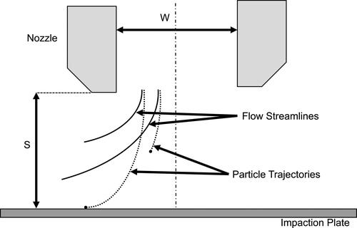
A typical inertial impactor, a schematic of which is shown in Figure 1, consists of a nozzle through which a particle laden flow enters to create a very short jet that is directed at a flat surface, referred to as the impaction plate or substrate. Large particles which have sufficient inertia will depart the flow streamlines and collect on the impaction plate whereas small particles follow the streamlines and are not deposited. To obtain a particle size distribution, impactors are organized into a cascade where the outlet of one impactor serves as the inlet to the next. Each impactor stage has a cutoff diameter which characterizes the minimum particle diameter captured at that stage. For an ideal impactor, all particles larger than the cutoff diameter are collected, and all those smaller than the cutoff diameter pass through, resulting in a plot of deposition versus diameter that would be a step function, but in reality is sigmoidal. The cutoff diameter is typically taken as the diameter at which 50% of the particles that enter the impactor deposit, $d_{50}.$ In a cascade, the impactors are sequenced from largest to smallest $d_{50}.$ Hence, each impactor (except for the first and last impactor in the cascade) captures particles that are larger than its cutoff diameter and smaller than the cutoff diameter for the previous stage. The difference between these two $d_{50}$ is the bin width for the resulting distribution. Once particle collection is over, the mass of particles collected at each stage can be measured and a histogram of particle diameters can be obtained.

Figure 1. Schematic of an inertial impactor. The nozzle diameter is $W$ and the nozzle-to-plate distance is $S.$

Strengths of impactors are their robustness, low cost, and simplicity of operation. A weakness of impactor cascades is that the number of bins in the particle size histogram (or distribution) is necessarily limited to the number of impactors in the cascade. While obtaining a histogram with ten bins is relatively straightforward, a histogram having, say, 100 bins can not be pragmatically obtained from an impactor cascade.

Typical particle impactors are operated so that $S/W\sim O(1)$ where $S$ is the distance from the nozzle exit to the impactor, and $W$ is the nozzle diameter. Under these conditions, the particle impaction pattern is disk-shaped as shown in Figure 2a. Fredericks and Saylor (2017) showed that when $S/W\mathrm{}\sim O(0.01),$ the particle impaction pattern is actually a fine ring, as shown in Figure 2b, and, importantly, the diameter of this ring is a function of the particle diameter, all other factors held constant (air speed, $S/W$). Specifically, Fredericks and Saylor showed that for $S/W=0.047:$ (1) $$D=-5.35Stk+14.94$$(1) where $D$ is the ring diameter, and $\mathit{Stk}$ is the Stokes number: (2) $$\mathit{Stk}=\frac{\rho d^{2}u}{9\mu W},$$(2) where $\rho$ is the particle density, $u$ is the nozzle exit velocity, and $d$ is the particle diameter (note that Equation (1)(1) $$D=-5.35Stk+14.94$$(1) was not actually presented in Fredericks and Saylor (2017), but rather was obtained by the present authors using the data from that reference). Equation (1)(1) $$D=-5.35Stk+14.94$$(1) shows that for the parameter space investigated by Fredericks and Saylor (2017), $D$ is a linear function of $\mathit{Stk}$ (proportional to $d^2$). If this remains true for a broad range of operating conditions, then it is possible for a single impactor to provide a particle size distribution. This could be done, for example, by obtaining the particle number density as a function of radial position on an impaction plate via, say, a laser based method. That plot of particle number density versus radial position could then be transformed into a particle size distribution using an equation like Equation (1)(1) $$D=-5.35Stk+14.94$$(1) where the radial location in the plot is translated into a particle diameter. If such a procedure could provide a ten-bin histogram from a single impactor, then a ten stage impactor cascade could potentially provide a 100-bin histogram, significantly improving the particle sizing resolution of impactor cascades.

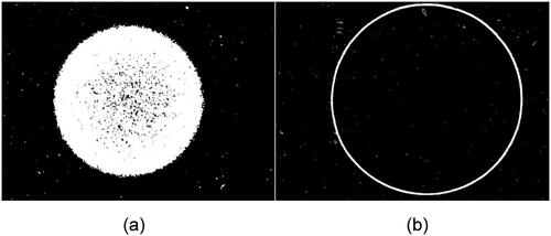
Figure 2. Difference between large and small $S/W$ impactor behavior: (a) Image of disk-shaped particle impaction pattern from an impactor having $S/W\sim 1.$ The diameter of the disk is 9.4 mm. (b) Image of a ring-shaped particle impaction pattern obtained from an impactor having $S/W\sim O(0.01).$ The ring diameter is 13.5 mm.

In this work we present experiments that enable us to generalize Equation (1)(1) $$D=-5.35Stk+14.94$$(1) , casting it in dimensionless form and showing how the dimensionless ring diameter is related to both $\mathit{Stk}$ and $S/W$ for a broader range of conditions than those presented in Fredericks and Saylor (2017); however we do not vary nozzle diameter or velocity and hence are unable to comment on any Reynolds number dependence. We also present simulations showing why a ring forms in the first place and conclude by discussing potential practical strategies for operating impactors so that sub-stage particle diameter sizing may be attained.

2. Experimental method

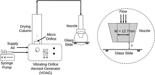
Particle impaction experiments using a single particle impactor were conducted for a range on particle diameters $d$ and $S/W$ to understand the dependence of these characteristics on the dimensions of ring shaped deposits. Figure 3 is a schematic of the experimental setup used. Monodisperse particles were generated using a variable orifice aerosol generator (VOAG - TSI Model 3450) and the particle laden flow was passed through a circular nozzle to create a jet that was directed at impactor plates. Disodium fluorescein (DSF) particles ranging from $d=2\mathrm{}\mu \mathrm{m}-10\mathrm{}\mu \mathrm{m}$ were used in this work. DSF is a water-soluble fluorescent dye having a density $\rho =1.6$ g/cm3. A DSF solution was made using a 50/50 water/isopropyl alcohol solvent. This solution was pumped at a fixed flow rate of 17.5 ml/hr into the VOAG using a syringe pump. The resulting monodisperse drops of DSF solution generated by the VOAG were carried up through a vertical drying column by dilution air which is house air having a relative humidity of 5% leading to evaporation of the isopropyl alcohol and water and leaving behind a monodisperse distribution of DSF particles. The dilution air was charge neutralized before entering the drying column by passing it through a Kr-85 neutralizer (TSI Model 3077A).

Figure 3. Schematic diagram of experimental setup.

The particle size is calculated from the concentration of the DSF solution and the liquid drop diameter according to: (3) $$d=C^{1/3}{d}_d$$(3) where $d$ is the particle diameter, $d_d$ is the drop diameter, and $C$ is the concentration (v/v) of the DSF solution. The frequency for generating the desired drop diameter is determined from: (4) $$d_d=(6Q/\pi f{)}^{1/3}$$(4) where $f$ is the frequency of the orifice and $Q$ is the liquid feed rate from the syringe pump.

The resulting dry monodisperse particles were carried by the dilution air through a nozzle consisting of three stages: an expansion plenum, a flow straightener, and the nozzle proper whose profile conformed to a fifth order polynomial following the design of Bell and Mehta (1988) which gives a flat velocity profile at the nozzle exit. The nozzle inner profile followed a fifth order polynomial contraction with the nozzle diameter decreasing from 43.2 mm at the inlet to 12.7 mm at the exit while moving 32.1 mm along the nozzle axis. Since the nozzle profile was curved the throat length was zero. The flange width was 6 mm and the angle of the external face of the nozzle outside of the flange area was ${42}^o$ from the horizontal. The jet diameter was $W=12.7$ mm and the velocity at the nozzle exit was $u=6.05$ m/s as measured by a TSI Velocicalc 9515 anemometer. As noted above, the particle diameter varied from $d=2\mathrm{}\mu \mathrm{m}-10\mathrm{}\mu \mathrm{m},$ giving a range in Stokes number $\mathit{Stk}=0.02-0.5.$ The nozzle was vertically mounted on a micrometer traverse to provide a downward facing jet oriented normal to the impaction plate and to allow control of $S/W,$ which was varied from 0.03 to 0.09 for for the experiments presented herein. The nozzle orifice was surround by a flat 5 mm flange which ran parallel to the impaction plate.

The impaction plates were $2″\times 1″$ glass slides coated with a film of petroleum jelly. The coating process involved dipping the slides in a 1:10 v/v petroleum jelly/heptane solution. Upon extraction from the solution, excess solution was wicked from the edge of the slide and the slide was then placed flat under a fume hood for 30 min to dry. This process, originally due to Sethi and John (1993), results in a uniform petroleum jelly coating. The glass slide was mounted on an optical lens holder which was fixed on a six axis micrometer stage located directly beneath the nozzle. The stage was used to ensure that the plate was oriented perpendicular to the nozzle axis. The aerosol impaction time for each run was 10 min which ensured sufficient particle deposition to enable imaging of the deposition pattern.

Once particle impaction was concluded, the glass slides were removed and imaged at 1X using a Canon Rebel T3i digital camera paired with a Canon MP-E 65 mm macro lens. Another set of 1X images of the coated slides with no particle deposition were taken as reference. The 1X images of the impaction slides with particle deposition were analyzed using an image processing routine written in the MATLAB programming environment. The geometric centers of the images were first obtained after which radial profiles of image intensity were obtained by averaging azimuthally at radial locations emanating outward from the center. The resulting radial profiles were $I_p$ for the images of particle impaction and $I_r$ for the reference slides. The radial profiles used here were the difference between the two: (5) $$I=I_p-I_r$$(5)

Subtracting out the reference image served to ensure that any background intensity and any spatial variation in background intensity did not affect the radial intensity profiles.

3. Results

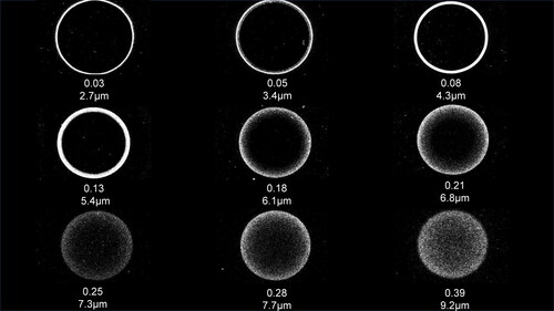
Figure 4 presents sample scaled images of the particle deposition patterns obtained for particle diameters ranging from $d=2\mathrm{}\mu \mathrm{m}-10\mathrm{}\mu \mathrm{m}$ and for $S/W=0.047$ (the value of $S/W$ used by Fredericks and Saylor (2017)). These 1X images of particle deposition were obtained by first converting the original color images to grayscale after which a threshold was obtained using Otsu’s method (1979). The threshold was used to transform the grayscale images to binary. In order to remove background noise, binary versions of the reference images were subtracted from the particle deposit images to obtain the final images. The figure clearly shows changes in ring diameter and thickness with increasing $d.$ This agrees with the results obtained by Fredericks and Saylor (2017).

Figure 4. Deposition patterns for particle diameters in the range $d=2\mathrm{}\mu \mathrm{m}-10\mathrm{}\mu \mathrm{m}$ and $S/W=0.047.$ Beneath each ring image is the Stokes number $\mathit{Stk}$ and the particle diameter $d.$ Note that for this fixed $S/W$ case, the ring thickness increases with $d,$ eventually approaching a solid disk.

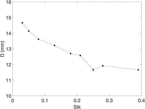
Figure 5 presents radial profiles of image intensity for the images presented in Figure 4. The information that we want from these profiles is the ring diameter $D,$ which we characterize as twice the radial location of the peak intensity. To reveal this more clearly, the profiles presented in Figure 5 are scaled to their peak intensity and replotted in Figure 6 which clearly shows that the peak location, and hence $D,$ increases with decreasing $\mathit{Stk}.$ This is further illustrated in Figure 7 where $D$ is plotted against $\mathit{Stk},$ revealing, roughly, a monotonic and linear decrease in $D$ with $\mathit{Stk}.$

Figure 5. Intensity versus $r$ for different $\mathit{Stk}$ at $S/W=0.047.$

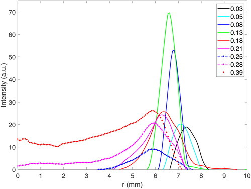
Figure 6. Scaled intensity versus $r$ for different $\mathit{Stk}$ for $S/W=0.047.$

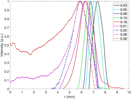
Figure 7. Plot of $D$ versus $\mathit{Stk}$ for the peaks presented in Figure 6 (note that $D$ is twice this radial location of the peaks seen in Figure 6). Here $S/W=0.047.$

Figures 4–6 show that the ring thickness $T$ also varies with $d$ and $\mathit{Stk}.$ This is further revealed in Figure S1 in the online supplemental information (SI), where $T$ is plotted against $\mathit{Stk}$ for the deposition patterns shown in Figure 4. Here we define $T$ as the radial distance between the two locations in the radial profiles where $I$ equals half the peak intensity. Figure S1 reveals a linear increase in $T$ with $\mathit{Stk}$ between $\mathit{Stk}=0-0.3$ followed by a sharp increase beyond $\mathit{Stk}=0.3.$

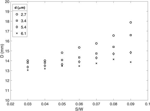
Figure 8 shows the results of a more detailed set of experiments where both $d$ and $S/W$ are varied, with $S/W$ ranging from 0.03 to 0.09 in increments of 0.01 and $d$ = 2.7$\mu \mathrm{m},$ 3.4$\mu \mathrm{m},$ 5.4 $\mu \mathrm{m}$ and 6.1 $\mu \mathrm{m}.$ Data obtained from the images presented in Figure 8 are presented in Figure 9 as plots of $D$ versus $S/W$ for the four particle diameters considered. These plots show that $D$ increases with $S/W$ and with decreasing $d.$ The plots also show that the change in $D$ with $S/W$ is greatest for the smallest particle diameter. A plot of $T$ versus $S/W$ for the four $d$ explored is also obtained from the images presented in Figure 8 and is presented in Figure S2 in the SI. These plots show that $T$ increases with $d$ but remains fairly constant with changing $S/W$ for any given $d.$ Given the relative insensitivity of $T$ to $d$ and $S/W$ when compared to the ring diameter $D,$ $T$ is not pursued further here as a means for obtaining particle diameter.

Figure 8. Experimentally obtained ring deposition patterns for a range of $S/W$ and $d.$ Note that at any given $S/W$ the ring diameter $D$ decreases with particle diameter $d$ (and hence with $\mathit{Stk}$). Note also that for the fixed range of particle diameters considered here, $D$ shows the maximum range for the largest $S/W,$ indicating that, for the parameter space explored here, detectivity should increase with $S/W.$

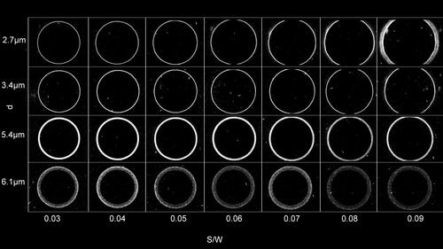
Figure 9. Plots of $D$ versus $S/W$ for $d$= 2.7 $\mu \mathrm{m},$ 3.4$\mu \mathrm{m},$ 5.4 $\mu \mathrm{m}$ and 6.1 $\mu \mathrm{m}.$

To present the relevant quantities in dimensionless form, we scale the ring diameter to the nozzle diameter: (6) $$D_s=D/W$$(6) and fit the data for $D_s$ to $\mathit{Stk}$ and $S/W$ using the cftool in the Matlab programming environment. Initially $D_s$ was fit using a form that was linear in $S/W$ and inversely proportional to $\mathit{Stk}$ which led to moderate results. Better results were obtained using the following form: (7) $$D_s=\frac{1.05Stk+0.17(S/W)-0.006}{\mathit{Stk}}$$(7)

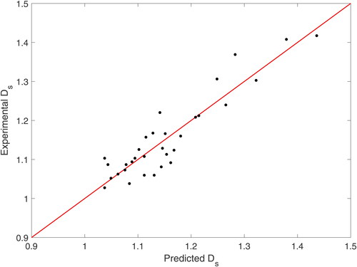
We note that Equation (7)(7) $$D_s=\frac{1.05Stk+0.17(S/W)-0.006}{\mathit{Stk}}$$(7) predicts the decrease in ring diameter with particle diameter ($\mathit{Stk}$), as did Equation (1)(1) $$D=-5.35Stk+14.94$$(1) , but unlike Equation (1)(1) $$D=-5.35Stk+14.94$$(1) is inversely proportional to $\mathit{Stk}.$ The accuracy of Equation (7)(7) $$D_s=\frac{1.05Stk+0.17(S/W)-0.006}{\mathit{Stk}}$$(7) is revealed in Figure 10 where the experimentally obtained $D_s$ are plotted against those obtained from Equation (7)(7) $$D_s=\frac{1.05Stk+0.17(S/W)-0.006}{\mathit{Stk}}$$(7) . A line of unity slope is included, and the data does not deviate significantly from the line.

Figure 10. Plot of the experimental ring diameter to that predicted by Equation (7)(7) $$D_s=\frac{1.05Stk+0.17(S/W)-0.006}{\mathit{Stk}}$$(7) . A line of unity slope is included (red). The $R^2\mathrm{}$ value for the fit is 0.9256.

4. Discussion

The results presented above show clearly via images and plots the impact of $\mathit{Stk}$ and $S/W$ on the ring thickness and diameter. Specifically, $D$ increases with $S/W$ and with decreasing $\mathit{Stk}.$ The relationship presented in Equation (7)(7) $$D_s=\frac{1.05Stk+0.17(S/W)-0.006}{\mathit{Stk}}$$(7) is favorably compared to the data in Figure 10, showing that knowledge of $\mathit{Stk}$ and $S/W$ should enable particle sizing within a single impactor stage (more on which, below). We note that to the extent that ($\mathit{Stk},S/W,D_s$) are the relevant dimensionless groups controlling the behavior of ring formation, Equation (7)(7) $$D_s=\frac{1.05Stk+0.17(S/W)-0.006}{\mathit{Stk}}$$(7) should predict behavior under other experimental conditions. However, it is likely that the Reynolds number $Re$ plays a role and hence a change in nozzle diameter or velocity may result in a change in Equation (7)(7) $$D_s=\frac{1.05Stk+0.17(S/W)-0.006}{\mathit{Stk}}$$(7) . Hence, future work should focus on experiments designed to extend Equation (7)(7) $$D_s=\frac{1.05Stk+0.17(S/W)-0.006}{\mathit{Stk}}$$(7) to include Reynolds number dependence.

The images and plots presented heretofore do not provide a mechanistic understanding of why rings are formed in some cases and why the ring diameter varies as it does. Clearly particle inertia plays the key role, but exactly how is unclear. To remedy this, we present here simulations of the particle trajectories for the conditions of the experiments presented. These were achieved by first simulating the flow field in Fluent assuming axisymmetry and using the exact dimensions of the nozzle used in the experiments, including the internal contours and the external structure, including the flat flange on the face and the angle of the external face of the nozzle outside of the flange area (see Figure 1). A multizone quadrilateral and triangular mesh was used. The mesh elements were $\sim 1\mathrm{}\mu$ m along the impaction plate and increased in size in the $y$ direction as the nozzle inlet was approached. No mesh element was larger than $30\mathrm{}\mu$ m . Once the flow field was obtained, trajectories were obtained for particles having diameters equivalent to those explored in the experiments. These trajectories were obtained starting at the nozzle inlet and solving for the force on the particle $F=F_d+F_g,$ the sum of the drag force $F_d$ and the gravitational force $F_g$ at each time step: (8) $$F_d=\frac{3\pi \mu V_{r}d}{C_c}$$(8) where $\mu$ is the absolute viscosity of air, $V_r=V-V_p,$ the particle velocity relative to the local flow velocity, and $C_c$ is the Cunningham correction factor (Hinds 1982): (9) $$C_c=1+\frac{\lambda }{d}[2.34+1.05\hspace{0.17em}\text{exp}\hspace{0.17em}(-0.39\frac{d}{\lambda }\left)\right]$$(9) where $\lambda$ is the mean free path of air. The gravitational force is: (10) $$F_g=mg$$(10) where $m$ is the particle mass and $g$ is the gravitational acceleration. The particle velocity was updated at each time step by integrating: (11) $$m\frac{d{V}_p}{dt}=F_d+F_g$$(11) to give: (12) $$V_p(i+1)=V_p\left(i\right)+\frac{(F_d+F_g)(\Delta t)}{m}$$(12)

These equations were integrated forward in time using a time step of $10^{-6}$ s. Here we follow the approach taken by Feng (2017) and presume that once the particle center is within one half diameter of the impactor plate, it stops and deposits, thereby ignoring the possibility of particle bounce. The significance of this assumption is discussed later. For all simulations, the jet exit velocity was the same as for the experiments ($u=6.05$ m/s). The flow field changes when $S/W$ changes, though the jet exit velocity was kept the same for all simulations (and for all experiments).

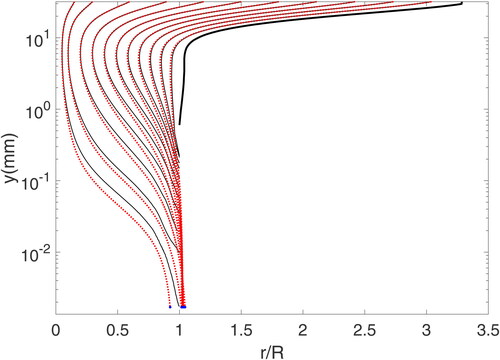
We first seek to explain the mechanism for the formation of disks versus rings. Here we present trajectories for the case where $d=7.7\mathrm{}\mu \mathrm{m}$ and $S/W=0.047$ followed by the case where $d=3.4\mathrm{}\mu \mathrm{m}$ and $S/W=0.047$ which correspond to the center image of the lower row and the center image of the upper row of Figure 4, respectively; these are cases resulting in a disk and a ring, respectively. Figure 11 shows the trajectories for the former condition. In this figure and in all subsequent particle trajectory figures, the particle trajectories are shown in dotted lines (red), and a streamline with the same starting location accompanies each trajectory and is presented as a thin solid line (black). The streamlines are arbitrarily terminated at $r/R=1$ to reduce clutter in the figures. A dot (blue) is used to denote the location of impact with the plate; note that this will not be located at $y=0$ since impact occurs when the center of the particle is one particle radius from the impaction plate. A dark outer black line shows the outline of the inner surface of the nozzle. Note also that these trajectories are presented with a logarithmic $y$-axis since the trajectories get too close together near the plate to be discerned in linear coordinates. For the case of Figure 11, it can be seen that the particle impact locations are spaced relatively uniformly though they are slightly closer together near the periphery than in the center. Hence, these simulations agree very well with the experiments which show in the center of the lower row in Figure 4 the image of a disk, though with a higher intensity at the edge than in the center.

Figure 11. Particle trajectories for $d=7.7\mathrm{}\mu \mathrm{m}$ and $S/W=0.047$ showing a relatively uniform deposition of particles which would correspond to a disk-like deposition pattern. Note that the $y$-axis is logarithmic to more clearly show the trajectories which cluster together in the region near the plate. Particle trajectories are in dotted lines (red) and streamlines are solid lines (black). The dark outer line is the nozzle inner surface.

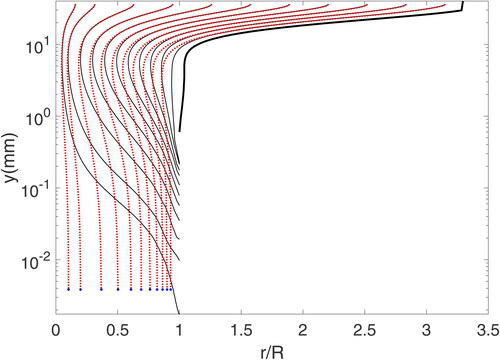
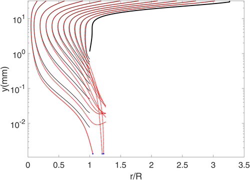
Figure 12 presents trajectories for conditions identical to those of Figure 11, except with $d$ decreased from 7.7 $\mu$ m to 3.4 $\mu$ m. The behavior here is clearly different from Figure 11, revealing particle deposition locations that are closely clustered together at a location very close to the nozzle periphery and with no particles deposited near the center. This agrees with the image presented in the center of the upper row in Figure 4 which is clearly that of a ring.

Figures 11–12 show that the primary difference between the large diameter (large $\mathit{Stk}$) behavior where disks are formed and the small diameter (small $\mathit{Stk}$) behavior where rings are formed is that for large $\mathit{Stk}$ the particles deviate from the streamlines much sooner than for the low $\mathit{Stk}$ case. When $\mathit{Stk}$ is big, in fact, the particles begin to deviate from the streamlines while still inside the nozzle. For small $\mathit{Stk},$ the particles follow the streamlines while inside the nozzle. But once they have left the nozzle exit, the particles fail to follow their streamlines and deposit at locations that are all relatively close to $r/R=1,$ resulting in a focusing of the particles and the formation of a ring. This is the cause of the ring formation for low $\mathit{Stk}$ and the cause of disk formation at high $\mathit{Stk}$ for the low $S/W$ conditions considered here.

Figure 12. Particle trajectories for $d=3.4\mathrm{}\mu \mathrm{m}$ and $S/W=0.047,$ showing the clustering of particles near $r/R=1,$ the nozzle edge, to form a ring. Particle trajectories are in dotted lines (red) and the streamlines are in solid lines (black). The $y$-axis is logarithmic.

It is important to note that $S/W$ is fixed in Figures 11–12 and the flow fields are identical as well. Hence, the difference in the patterns seen as $d$ decreases from 7.7 $\mu$ m in Figure 11 to 3.4 $\mu$ m in Figure 12 is due not to the flow field and only to the difference in particle inertia. Accordingly, we now look at the change in trajectories as $S/W$ is changed while keeping the particle diameter constant. We note that changing $S/W$ while keeping the jet exit velocity $u$ constant still results in a new flow field due to the change in flow resistance resulting from different $S/W.$ Hence, while keeping $u$ constant and varying $S/W,$ what is really changed is the flow field, though the overall magnitude of the flow may be thought of as the same. In Figures 13 and 14, we present trajectories for the conditions used to obtain the images in the upper left hand and upper right hand corners of the image matrix in Figure 8. Here, $d=2.7\mathrm{}\mu$ m and $S/W$ is increased from 0.03 to 0.09. The particle trajectories obtained for these two conditions are presented in Figure 13 for $S/W=0.03,$ and in Figure 14 for $S/W=0.09.$ The $y$-axis is kept the same in these two figures, and the change in $S/W$ can be seen in the change in the vertical position of the nozzle exit.

Figure 13. Particle trajectories for $d=2.7\mathrm{}\mu \mathrm{m}$ and $S/W=0.03.$

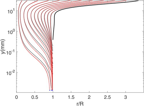
Figure 14. Particle trajectories for $d=2.7\mathrm{}\mu \mathrm{m}$ and $S/W=0.09.$

The simulations show the same results as do the experiments, namely that for the small $S/W$ case, the ring diameter $D$ is smaller and the ring thickness $T$ is thinner than the large $S/W$ case. Specifically, for $S/W=0.03,$ the particles all deposit at $r/R<1$ but close to $r/R=1$ and close to each other, while for $S/W=0.09,$ the deposition locations are all at $r/R>1$ and are deposited over a larger range. The cause of the different behavior is due to the different flow fields. The streamlines are forced to turn radially outward beginning at a smaller $y$ for the smaller $S/W$ case which causes the particles to travel in a straighter direction, impacting at a location just inside the nozzle radius and with a limited range of deposition locations than is the case for the larger $S/W$ case.

A comparison between the values of $D$ obtained in the experiments and simulations is presented in Table 1 and which shows reasonable agreement between the two. The values of $D$ from the simulations are calculated by obtaining deposition locations for 210 equally spaced particle trajectories starting 0.05 mm from the nozzle axis and moving toward the nozzle edge. The radial deposition locations obtained from these trajectories are binned in bin sizes of 0.05 mm and counted. The bin with maximum counts is noted and twice the radial location of this bin gives the ring diamter ($D$) for the case in consideration.

Table 1. Comparison of experimental and simulation $D.$

$d(\mu m)$	$S\mathrm{tk}$	$S/W$	$D$ (mm)
			Experiment	Simulation
2.7	0.03	0.03	13.7	12.6
2.7	0.03	0.09	17.5	16.6
3.4	0.05	0.047	14.3	13.0
7.7	0.28	0.047	11.9	10.9

The above discussion shows how particle inertia and the flow field interact to cause the formation of rings and how these two factors control the way in which $D$ changes with $\mathit{Stk}$ and $S/W.$ It should be noted that other factors can impact the resulting patterns. For example, Feng (2017) shows how the internal geometry of the nozzle can affect the deposition pattern. Additionally, particles may bounce upon impact and not deposit, or deposit at an outter radial location, effects that are not included in the simulations presented here. Finally, given that in many cases particle deviation from streamlines occurs when the particles are very close to the wall and where velocity gradients are highest, effects such as the Magnus effect (Rubinow and Keller 1961) or Saffman forces (Saffman 1965, 1968) may be important. Including these effects may result in greater agreement between the simulations and the experiments. These issues are left as future work.

While development and demonstration of a practical implementation of the method presented herein goes beyond the scope of this article, possible approaches to such an implementation are now discussed. The ring images presented herein were for samples of monodisperse particles, an approach which reveals clear rings and which is useful in revealing the physics at hand. However, in an actual cascade impactor, the particles entering will be polydisperse and so, should one use the low $S/W$ approach described here, the resulting particle impact pattern would not be a set of rings, but rather a smooth variation in intensity with radius on the impactor surface. To obtain a particle size distribution for such a polydisperse flow of particles in a single stage of an impactor having small $S/W,$ the impaction pattern obtained would be first imaged and a radial intensity plot ($I$ versus $r$), would be obtained like that obtained in Figure 5 for the monodisperse case (and which would obviously show a broader structure rather than the sequence of peaks shown in the figure). Next, using Equation (7)(7) $$D_s=\frac{1.05Stk+0.17(S/W)-0.006}{\mathit{Stk}}$$(7) , the radial intensity plot would be translated into a plot of intensity versus particle diameter $d.$ To relate the intensity to number of particles deposited, $I$ would be scaled to $d^2,$ invoking the assumption that the scattered intensity scales as projected particle area, which is valid for the case where the particle diameter is larger than the wavelength of light. The resulting plot of $I/d^2$ versus d would require a calibration since $I/d^2$ is proportional to, but not equal to the particle surface density $n.$ To relate $I/d^2$ to the actual number of particles deposited per unit area on the plate, one could first run the impactor using a range of monodisperse particles of known diameters for a short period of time and using a microscope to visually count the number of particles in a given area. Images of this calibration run would enable a relationship between $I/d^2$ and $n$ allowing one to transform the plot of $I/d^2$ versus $d$ to $n$ versus $d.$ The final step would require a transfrom of $n$ the number of particles deposted per unit area to $N$ the number of particles per unit volume in the incoming flow. This last step would require the collection efficiency as a function of particle diameter for the range of diameters collected by the impactor state. Relationships and experimental data exist for the particle collection efficiencies of impactors, but none for the low $S/W$ conditions explored here. Hence another calibration would be required to obtain this final step. This calibration could be achieved using two optical particle counters, one each at the impactor inlet and outlet. The collection efficiency is likely to change with $d$ and $S/W$ and so the necessary calibrations could be non-trivial. However these could also be obtained computationally via simulations similar to those presented herein; indeed, precisely this was done by Feng (2017).

An important aspect of the particle size distribution obtained by the method presented here is the resolution in particle diameter attained. To estimate this resolution, we use a full-width half-max metric, which is to say that we claim we can separate particle diameters whose intensity versus deposition location plots, like those in Figure 6 intersect at, or less than, one-half the peak value. For the discrete particle cases examined in Figures 5–6, this condition is met for the particle diameters of 2.7 $\mu$ m and 6.8 $\mu$ m, giving a resolution of 4.1 $\mu$ m for the $S/W=0.047$ case. This resolution is improved to 2 $\mu$ m for $S/W$ of 0.09, where the particle diameters of 3.4 $\mu$ m and 5.4 $\mu$ m can be separated. This is shown in Figure S3 of the SI. However, for $S/W=0.03,$ it is not possible to differentiate the peaks for particle diameters between 2.7 $\mu$ m and 6.1 $\mu$ m as shown in Figure S4 of the SI. Thus, resolution increases with $S/W,$ at least for the $S/W$ = 0.03 to 0.09 range explored here. In the previous section, it was also demonstrated that detectivity of particle diameter increased with $S/W,$ making large $S/W$ especially useful. Of course continued increase in $S/W$ will eventually result in behavior that reverts to the large $S/W\sim O(1)$ situation and the formation of a filled disk and decreased performance. Hence there must be an optimum $S/W$ greater than the maximum of 0.09 explored here.

Of course the particle size resolution demonstrated here is not superb, and in its current form, implementation of this technology would not result in significant sub-stage particle size resolution in an impactor cascade. At the same time, we hasten to note that we have not optimized the parameters explored here in any way. The abovementioned optimum $S/W$ being just one example of a parameter that could be optimized. It is likely that further exploration of other parameters, such as Reynolds number, and more sophisticated control of operating conditions will increase resolution.

Finally, we note that in the above discussion describing the steps needed to obtain a particle size distribution from a small $S/W$ plate, we began with the assumption that taking an image of the plate would be the first step. However other approaches could be considered. The typical approach used to obtain the number of particles on the impactor surface in a traditional cascade impactor is to simply weigh the plate before and after sampling. A similar approach could be used with the low $S/W$ method presented here if a plate could be manufactured consisting of several tightly fitting rings. Each of the rings could be weighed before sampling and then fit back together to create a plate. After deposition, the rings could be disassembled again, taking care not to remove particles in the process and then each ring could be re-weighed. A challenge to such an approach would be the accidental addition or subtraction of particles during the assembly/disassembly of the plate. Also, a different optical approach could also be used. For example, the beam of a moderate power HeNe laser could be expanded and collimated to a diameter equal to that of the impactor plate, which would be made of glass in this implementation. An image of the plate obtained by a camera having the same optical axis as that of the laser, but located on the other side of the glass plate and facing the laser, could be acquired. If the particle deposition period was short enough that one could assume no portion of the plate was completely saturated with particles (i.e., no region had more than one layer of particles), then the difference between the intensity of the image, and that of an image obtained from a similar plate without particles would be linearly related to the area fraction covered in particles. Using the expected particle diameter obtained from Equation (7)(7) $$D_s=\frac{1.05Stk+0.17(S/W)-0.006}{\mathit{Stk}}$$(7) , this could be translated into a particle number density. Of course this approach would have its own problems as well. One would have to assume that a particle completely occludes the laser light. Also, particle diffraction issues could impact the results.

5. Conclusions

Experiments and computer simulations of particle impaction were conducted for small $S/W$ impactors ranging from $S/W=0.03-0.09$ for micron scale particles. The small $S/W$ conditions favor the formation of rings whose diameter $D$ are shown to be related to both $S/W$ and $\mathit{Stk},$ enabling the development of an equation for $D$ in terms of $\mathit{Stk}$ and $S/W.$ This relationship allows one to ascertain the diameter of a particle deposited at a particular radial location given that $S/W$ is known. Methods by which these new results may be used to obtain sub-stage particle sizing in inertial impactors was described. Future work should focus on further experiments and simulations to quantify the collection efficiency as a function of $\mathit{Stk}$ and $S/W$ for small $S/W,$ to ascertain any Reynolds number dependence, and to quantify the effect of particle bounce, and Saffman and Magnus effects on the relationship between $D$ and $\mathit{Stk}$ and $S/W.$

Additional information

Funding

This material is based upon work supported by the National Science Foundation under Grant No. 1804304.

References

- Bell, J. H., and R. D. Mehta. 1988. Contraction design for small low-speed wind tunnels. Technical report, NASA.
- Craig, R. L., P. K. Peterson, L. Nandy, Z. Lei, M. A. Hossain, S. Camarena, R. A. Dodson, R. D. Cook, C. S. Dutcher, and A. P. Ault. 2018. Direct determination of aerosol pH: Size-resolved measurements of submicrometer and supermicrometer aqueous particles. Anal. Chem. 90 (19):11232–9. doi:10.1021/acs.analchem.8b00586.
- Dzubay, T. G., R. K. Stevens, and P. L. Haagenson. 1984. Composition and origins of aerosol at a forested mountain in Soviet Georgia. Environ. Sci. Technol. 18 (11):873–83. doi:10.1021/es00129a012.
- Feng, J. Q. 2017. A computational study of particle deposition patterns from a circular laminar jet. J. Appl. Fluid Mech. 10 (4):1001–12.
- Fredericks, S., and J. R. Saylor. 2017. Ring-shaped deposition patterns in small nozzle-to-plate distance impactors. Aerosol. Sci. Technol. 52 (1): 30–37. doi:10.1080/02786826.2017.1377829.
- Hinds, W. C. 1982. Aerosol technology: Properties, behavior, and measurement of airborne particles. New York, NY: Wiley-Interscience.
- Juozaitis, A., K. Willeke, S. A. Grinshpun, and J. Donnelly. 1994. Impaction onto a glass slide or agar versus impingement into a liquid for the collection and recovery of airborne microorganisms. Appl. Environ. Microbiol. 60 (3):861–70. doi:10.1128/aem.60.3.861-870.1994.
- Kulkarni, P., P. A. Baron, and K. Willeke. 2011. Aerosol measurement: Principles, techniques, and applications. 3rd ed. Hoboken: Wiley.
- Marple, V. A. 2004. History of impactors - The first 110 years. Aerosol. Sci. Technol. 38 (3):247–92. doi:10.1080/02786820490424347.
- Marple, V. A., D. B. Kittelson, K. L. Rubow, and C. P. Fang. 1986. Methods for the selective sampling of diesel particulate in mine dust aerosols. NIOSH Technical Report NTIS: PB 88-130810, NIOSH.
- McMurry, P. H., and X. Q. Zhang. 1989. Size distributions of ambient organic and elemental carbon. Aerosol. Sci. Technol. 10 (2):430–7. doi:10.1080/02786828908959282.
- Mora, J. F. D. L., S. V. Hering, N. Rao, and P. H. McMurry. 1990. Hypersonic impaction of ultrafine particles. J. Aerosol. Sci. 21 (2):169– 87. doi:10.1016/0021-8502(90)90002-F.
- Otsu, N. 1979. A threshold selection method from gray-level histograms. IEEE Trans. Syst, Man, Cybern. 9 (1):62–6. doi:10.1109/TSMC.1979.4310076.
- Rubinow, S. I., and J. B. Keller. 1961. The transverse force on a spinning sphere moving in a viscous fluid. J. Fluid Mech. 11 (03):447–59. [Database] doi:10.1017/S0022112061000640.
- Saffman, P. G. T. 1965. The lift on a small sphere in a slow shear ow. J. Fluid Mech. 22 (2):385–400. doi:10.1017/S0022112065000824.
- Saffman, P. G. T. 1968. The lift on a small sphere in a slow shear ow - Corrigendum. J. Fluid Mech. 31:624.
- Sethi, V., and W. John. 1993. Particle impaction patterns from a circular jet. Aerosol. Sci. Technol. 18 (1):1–10. doi:10.1080/02786829308959580.
- Yoon, K. Y., C. W. Park, J. H. Byeon, and J. Hwang. 2010. Design and application of an inertial impactor in combination with an ATP bioluminescence detector for in situ rapid estimation of the efficacies of air controlling devices on removal of bioaerosols. Environ. Sci. Technol. 44 (5):1742–6. doi:10.1021/es903437z.