“Invisible bias” in the single particle soot photometer due to trigger deadtime

Abstract

The Single Particle Soot Photometer (SP2) is an instrument for quantifying the refractory black carbon (rBC) mass and microphysical properties of individual aerosol particles. Under substantial aerosol loadings, the SP2 data system can bias rBC concentration measurements low by 40% at a particle rate of 25,000 particles s⁻¹, with significant bias (∼4%) even at only ∼2000 particles s⁻¹ without any explicit record of this “invisible” effect. Here we present information about the SP2 algorithm for storing individual particle data and its susceptibility to generating this bias, which is strongly sensitive to user choices of various SP2 operational parameters. A method to directly measure this bias, and an approach to assessing it from analysis of saved data is provided, and evaluated with laboratory-generated aerosol and against theory. Finally, recommendations for sampling aerosol and quality-assuring stored SP2 data with this bias in mind are provided.

Copyright © 2022 American Association for Aerosol Research

EDITOR:

• Hans Moosmüller

1. Introduction

The Single Particle Soot Photometer (SP2, Droplet Measurement Technologies, Inc, Boulder, CO) is primarily used to quantify the refractory black carbon (rBC) mass concentration of aerosols. It can also quantify the rBC size distribution, and the total particle optical size of rBC-containing particles. Over the last decade and a half, the SP2 has been deployed to survey the atmosphere in many different regimes, from land, sea, and air, has been used in laboratory measurements, and was applied to snow, ice, rain, and sediment sample characterization. Although SP2 performance has been repeatedly evaluated (Zanatta et al. 2021; Laborde et al. 2012; Cross et al. 2010; Schwarz et al. 2010; Slowik et al. 2007), there are still unresolved issues associated with its calibration and the analysis of the complex data it produces, especially for conditions that are not typically experienced in “normal” operation. Here we explore a specific source of bias that is detectable under normal operation and can become a dominant uncertainty under heavy particle concentrations such as occur in the atmosphere near strong sources, for example smoke from open burning, in some laboratory settings, and in measurements of condensed samples made using efficient nebulizers. Specifically, we focus on the effects of high concentrations of non-rBC-containing particles on rBC concentration measurements. Non-rBC-containing particles typically dominate accumulation mode number concentrations in the ambient and in laboratory measurements of aerosolized liquid samples of snow, rain, and ice. The bias is a consequence of the algorithm (the “triggering algorithm”) used to select raw data for storage and later analysis. Note that we do not address cases where the rBC concentrations themselves are so high as to themselves generate significant bias. First, we describe the data acquisition system of the SP2, with a focus on the triggering algorithm and its behavior under load with high rates of detection of rBC-free particles. Second, we describe an approach to assessing, through post-acquisition analysis of data, the likelihood for and magnitude of the bias associated with the triggering algorithm in un-recorded rBC-containing particles. Third, we present a measurement strategy to directly constrain the bias and use it in laboratory tests using known external mixtures of rBC-containing and rBC-free aerosol. We use these tests to explore the dependence of the bias on SP2 operational configuration and to evaluate the performance of the post-acquisition bias assessment. Finally, we provide suggestions for recognizing and minimizing SP2 deadtime bias driven by high rBC-free particle loads.

2. SP2 data acquisition system

The SP2 has four detectors that image the interactions of an air stream with an intense, intra-cavity 1064 nm laser. The specific configuration of these detectors can vary, but typically two detectors measure different bands of visible light generated by particles incandescing in the laser, a single detector quantifies elastically scattered laser light (the “scattering” detector), and last a, differential detector sensitive to scattered laser light provides a fixed location reference for particle position in the laser (the “position sensitive detector”). Signals from these four detectors are continuously and synchronously recorded at 5 MS/s to a memory register of length 1,000,000 points (on each channel). Each detector signal can be either AC or DC coupled to the digitizer—i.e., either with or without the low-frequency background signal on a channel removed. We originally used AC coupling with the scattering channel to avoid large DC signal offsets associated with background laser light in the SP2 without the need for additional electronics. Note that some models of the SP2 have high and low-gain detection of these four channels and the resulting 8-channels of detection are only digitized at 2.5 MS/s. The data storage algorithms used are common to both systems and the workings of the triggering algorithm are similar in all SP2 models and independent of digitizer sample rate or software version. For the rest of this work, we will only refer to the 5MS/s system that we have tested and present here—we expect 2.5 MS/s results to translate appropriately. Approximately each 0.2 s the contents of the memory register are transferred to a data buffer used for scanning for individual particle detections; it is the identification algorithm, or “triggering algorithm” for choosing each “packet” of data associated with each particle transit across the laser that is the source of the bias discussed here. To avoid coining new terms, the nomenclature of the SP2 user manual (Version 4.0, Revision F, Droplet Measurement Technology) is adopted here.

To first order, the triggering algorithm simply scans for an occasion (a “trigger event” or “threshold exceedance”) in which a signal increases past a threshold value that is either set by the user or calculated via a user-defined offset from the background level. One or two channels of data can be searched for this kind of event by the SP2 data acquisition system. In the SP2’s common configurations, the primary channel to be searched is typically associated with light scattered out of the laser by particles with either the scatter or position sensitive detector channel. This allows storage of data associated with all aerosol particles optically large enough to generate a sufficient signal to exceed the threshold value; the full continuous data record is not stored because it would quickly become unmanageably large. The secondary channel typically used for triggering is the highest-gain incandescent visible-light channel, to allow detection of particles that incandesce without scattering enough light to trigger the first threshold (namely small refractory black carbon (rBC) particles with very little additional material internally mixed with them). A benefit of having two different triggering channels is that this can allow preferred storage of particles by type (purely light-scattering, or incandescent). This is very useful in cases where non-incandescent particles are not a science target, as is the case commonly in laboratory-aerosolized rain, snow, sediment, and ice samples measured with an SP2 (Zanatta et al. 2021; Katich, Perring, and Schwarz 2017) and in some cases in the ambient (notably when other dedicated instrumentation for total, rather than rBC-containing, aerosol is available). Note that non-incandescent particles are used to determine (via the relationship of the scattering signal and the position sensitive detector signals) the speed of particles through the SP2 laser, and the relative position of the position sensitive detector reference and the center of the laser; this is critical information for obtaining microphysical information about rBC-containing particles via the leading-edge only (“LEO”) fitting technique (Gao et al. 2007), especially for airborne use of the SP2 where particle speed typically varies with aircraft altitude, etc.

Each trigger event identifies a short window of data for possible storage to disk and later analysis. User-specified numbers of “pre-trigger datapoints” and “total data points” define the initial position (in time) of this window relative to the trigger event, and the window’s total length, respectively. The user defines these quantities according to need. For example, for LEO-fitting, a well-defined signal background is a requirement, so a longer pre-trigger and wider total data window segment are useful. A study of particles more slowly transiting the laser than typical would also need a longer total data window. For this reason, we deal with the case where the pre-trigger length is approximately ½ the window total time; this keeps the particle signals approximately centered in the window and provides leading and trailing measurements of scattering background valuable for LEO. For detection only of rBC-containing particles, without associated scattering information or without LEO-fitting, a shorter window of data and pre-trigger length are needed, reducing data storage requirements and easing the problems that we explore here for heavy particle loads to some degree. Note that the NOAA SP2 is often operated with the scatter-particle trigger threshold significantly higher than its minimum reasonable value to reduce data space requirements and computational load on the computer while still recording larger scattering particles useful for determining LEO parameters (laser width, position-sensitive detector location). We prefer to trigger scattering particles off of the position sensitive detector signal (with a negative leading lobe) such that the trigger occurs when each particle is at a near-fixed depth in the laser beam, independent of particle size. This has additional benefits for deadtime sensitivity at extreme particle rates.

2.1. SP2 triggering algorithm

Here we present the specifics of the SP2 triggering algorithm (“TA”) that defines the data identified as containing particle information for possible storage to disk, and eventual analysis. Note that, in general post-analysis, the TA performance cannot be evaluated in an absolute sense because only the stored data record is available. For this reason, we refer to the bias arising from the TA as “invisible.” The SP2 can be configured to record complete “snapshots” of digitizer data, not subject to the TA, at fixed intervals. Due to storage space limitations, however, these “raw” data records are typically configured a priori to be quite small (e.g., 4000 consecutive buffer points, equivalent to 10–20 individual particle detections once per minute) and are not very useful to the evaluation relevant here. In general implementing storage of such snapshots can be valuable for troubleshooting.

The TA identifies windows of high-speed data for consideration for storage. Additional constraints, applied separately from the algorithm, determine if individual windows are actually stored for post-acquisition analysis: (1) optionally, incorrectly sampled (i.e., “wide”) particles are not recorded (2) optionally, a fixed fraction of trigger events are discarded to reduce data storage requirements (3) very limited storage space requires a strongly reduced (e.g., 1%) rate of storage (4) particle type (e.g., scattering particle or incandescent particle) can be used to make selective reductions in storage space—for example we often only record 20% of the scattering-particle-only windows, but 100% of those with signal on the triggering incandescent channel (5) minute-by-minute options for data saving are implemented. Constraint 1 adds evaluation of the length of time that a signal is elevated above a threshold; if it is too long (e.g., the particle is “wide,” as determined by the last point in a window being elevated above the threshold) the whole event is discarded. Under heavy particle loadings, when multiple particles can cross the SP2 laser within a single trigger window, this constraint would lead to huge reductions in data stored to disk. As this kind of event often arises from random particles floating in the SP2 optical chamber, but not entrained in the normal sampling process, they are quite rare under correct sampling conditions, and hence we only consider the case in which this option is disabled (NOAA SP2s have never been operated with this option enabled, and we do not recommend its use ever). Constraints 2–5 intentionally reduce the amount of data stored. As these constraints do not influence the way that the TA identifies valuable data windows, we do not focus on them, but they must always be accounted for in interpreting data stored to disk.

The TA is simple when applied to a single channel: first, the earliest threshold exceedance on the channel is identified in a buffer of data (if one exists). The window of data associated with this event is identified, and then the search for the next trigger event begins not at the end of the window, but rather at “pre-trigger points” after the end. This serves to avoid the possibility that any portion of data could be duplicated in two different triggered windows saved to disk, possibly resulting in overcounting of particles. If the search started immediately at the end of a window and a threshold exceedance was immediately found, the pre-trigger points would extend back into the previously identified window. A consequence of this approach, however, is that any threshold exceedance occurring within those “pre-trigger points” immediately following a triggered window will not independently trigger storage/evaluation. Explicitly, each trigger event is associated with deadtime of pre-trigger points length, and any threshold-exceedance within that deadtime will not trigger storage to disk—this is one source of bias (“post-trigger deadtime”) that we explore in more detail below. Note that if the data in this period is indeed written to disk due to another trigger event, it would no longer generate deadtime in the SP2.

When a secondary channel for triggering is included in scanning of a buffer of data, the algorithm is extended as follows: from a start point in the buffer (initially the start of the buffer) it first searches for a trigger on the primary channel until it finds one, and then searches for a secondary-channel trigger. The trigger that occurred earlier in the buffer identifies the triggered “window” of data, and the new start point to begin the search for the next trigger (i.e., after the window of data for the found trigger and an additional “pre-trigger number” of points). The search continues on the earlier triggered channel (whichever one it is) until the next threshold exceedance is found. This repeats until no triggers are found between the starting point for the search and the end of the buffer. When both triggers are activated by a single particle—for example a rBC-containing particle that generates a threshold exceedance on both primary and secondary channels, the later trigger within the window is discarded. One small difference between the software tested here and the version 4 now provided by Droplet Measurement Technology, Inc., affects a small portion of data at the end of the buffer scan. If it is too short to fill a window of data, it is discarded by the NOAA software used here, but included in the next scan in the version 4 system. This represents, at most under conditions tested here, <0.1% deadtime, and hence is ignored. Just as in the single-triggering channel case above, at low particle rates, the situation is described well as for rates with rare coincident particles with the pre-trigger length largely determining the deadtime per threshold exceedance (pre-trigger points per trigger). Note that “auto-thresholding” is a SP2 option that adjusts the threshold based on low-frequency signals from the triggering channels. Auto-thresholding typically occurs at ∼1 min or slower time scales, and is untested under very high loadings. Hence, we do not explore its potential influence on bias, and do not recommend auto-thresholding for situations where high loadings could be experienced.

The difference between the thresholds (Threshold 0 and Threshold 1) and baseline signals for each channel determines the smallest signal from each channel that is believed to unequivocally indicate a particle interacting with the laser. Triggers only occur on signals transiting from below-threshold values to those higher than the threshold; further the “trigger hysteresis” parameter defines the number of signal counts that the signals must drop below their respective thresholds before a new trigger can be identified. Generally, the trigger hysteresis parameter is set to a very small value (e.g., we use 5 in the 4-channel SP2) and is not an important factor in influencing bias.

2.2. The influence of high scatter-particle concentrations on the performance of the triggering algorithm

Under light particle loads, in which only negligible numbers of particles cross the laser beam in close succession on the timescale of the windows of data being stored, the TA generates bias adequately predicable via existing theory (as discussed below). Under increasing loads, two problems associated with the algorithm become more important, and are shown in Figure 1. First, (left panel) the “post-trigger deadtimes” become more frequent, resulting in increasing bias until particle rates are so high that the data associated with the unscanned periods is stored due to random “just in time” threshold exceedances (as in the example shown in the figure) and bias begins to decrease. At low particle rates, this is a simple situation that has been dealt with many years ago in the context of detectors for nuclear particle experiments for “non-paralyzable” deadtime situations, in which trigger events in the deadtime period do not extend the deadtime or co-incident triggers are rare (Feller 1948). At detection rates without significant co-incidence of arrivals, the deadtime bias (because the arrival time of rBC-containing particles is expected to occur in a random Poisson distribution) is merely the fraction of sampling time that is associated with this lack of sensitivity to new threshold exceedances. For a scatter particle rate of R_S per second, and a pre-trigger length of τ seconds, the relative bias, B_rel, is (1) $$B_{\mathit{rel}}=\mathrm{}-R_S*\tau$$(1) For example, with a pre-trigger length of 100 measurements corresponding to a τ of 20 µs at a 5 MS/s digitization rate, and a scatter particle rate of 5000/s (e.g., 2500 scattering particles/cc sampled at 2 cm³ s⁻¹ = 120 vccm), we would expect a relative bias of −0.1—i.e., a 10% low bias in the measurement of relatively low rates of rBC-containing particles affecting rBC number and mass concentrations. However, at particle higher rates this simple treatment fails. One failure occurs, as above, because this deadtime only generates bias if the data is not written to disk for later analysis. The probability of effective deadtime decreases because of the higher likelihood for a quick threshold exceedance occurring soon after the algorithm search under heavier loads. Also, at higher particle rates, a different source of deadtime can become important.

Figure 1. Left: An incandescent particle that transited the laser within the “pre-trigger number of points” (hatched area) after a triggered window—this did not generate a trigger, but the second particle (an incandescent particle at ∼ point 200) did. If the second particle did not cross the laser within this window, the first particle’s signals would not have been saved. This example was recorded from actual aerosol, and reflects the “non-paralyzable deadtime” situation. Right: synthetic data to represent the case of multiple particles crossing the laser in rapid succession, maintaining a scatter signal above threshold, and thus disabling triggering of a threshold exceedance event on the incandescent channel. The solid shaded area represents a trigger and its associated window, followed by the hatched area representing pre-trigger points beyond that window. Beyond that, deadtime is extended. This represents the “paralyzable deadtime” situation. Ambient data could not be used because in this case only the original window (solid shading) would have been saved by the SP2.

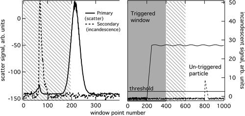
The second effect relevant to deadtime is shown in Figure 1, right panel: elevated signals on either trigger channel delay identification of new particle events until signals decrease sufficiently for the triggering to “reset”—as described in Sec. 2.1, the signal must drop below a threshold less a small hysteresis value before an exceedance can again be observed. This second case can become important when many particles cross the laser in close succession, thereby maintaining signals on either triggering channel above its respective threshold; when the background signal on a triggering-channel increases above the threshold value for that channel; or when a threshold is set to a value below the minimum signal on a channel. The last two conditions disable all triggering of detections on both channels indefinitely, even if the condition exists on only one channel. Clearly, the requirement for “positive slope triggering” across thresholds can contribute strongly to triggering bias, as it can lead to this “paralyzable deadtime” behavior (Evans 1955), in which frequent co-incidence of particle arrivals can extend deadtime greatly beyond the pre-trigger time for each triggered event in the SP2. This is the case under heavy loads and in certain configurations of the instrument, and is very relevant to this second issue under heavy particle loads. In fact, it can lead to complete loss of data! However, this does not always apply in the SP2 even with near-continuously arriving scattering particles. For example, the position-sensitive detector generates both positive and negative voltages around its baseline, and so, when used for triggering of scattering particles, does not lead to the limit of the paralyzable case with complete data loss. Note, too, that SP2 sensitivities associated with the physical process of detection under heavy loads can also affect detection under extreme aerosol loads (for example, see Zanatta et al. 2021, in which high salt concentrations quenched rBC incandescence); these possibilities are not explored here.

3. Evidence of trigger bias in SP2 data written to storage

Here, we describe an approach to assessing, in post-acquisition analysis of data, the likelihood that the triggering algorithm was significantly biased in recording particles for conditions where the simple situation described by Equation (1)(1) $$B_{\mathit{rel}}=\mathrm{}-R_S*\tau$$(1) cannot simply be trusted. Both biases that were discussed above are consequences of particles crossing the SP2 laser with little or no separation in time, hence our approach quantifies related information: first, the number fraction of particles recorded that show evidence of additional near-simultaneous contamination (“fraction contaminated,” F_C), and second, the fraction of each buffer’s data associated with triggered windows (“fraction triggered,” F_T). F_C is calculated on a per-buffer (i.e., 0.2 s data record) basis. It is derived from only the early scatter-channel data in each saved event: data that is included in the window under normal circumstances to provide a baseline for signals before a particle produces any signal in the detectors. This portion of the data is scanned for evidence of an un-triggered particle—a “contamination” generated by either a rBC-free or rBC-containing particle. Such events can only occur through the near-simultaneous sampling of at least three particles (the first that triggered the previous window, the second that occurred in the “pre-trigger” portion of the focus event that is not scanned, and the third that causes the triggering and saving of the focus event). The amount of signal change on the scatter channel necessary to be considered as contamination was chosen so as to provide sensitivity to the smallest particles clearly observable given noise and stability of the primary trigger channel. F_C of 1 indicates that every window written to disk showed evidence of additional particles before the trigger event; F_C of 0 indicates that none did.

F_T is also calculated on a per-buffer basis to avoid duty cycle issues, and represents the fraction of time in each 0.2 s buffer read that was associated with triggered window events (which is effectively not deadtime, as the data was written to disk). F_T is low when particles are few and far-between, and increasing with particle concentrations and particle passage-rates through the laser. F_T also depends on the length of each window. A fraction of 1 indicates that every measurement in the buffer was associated with a triggered window, so no data could be lost unintentionally, and there is no possibility for extensive deadtime. This is nearly an impossible fraction to achieve in practice. Fractions near 0 indicate, most probably, a low rate of particles crossing the laser (ideal conditions for the SP2). However, a fraction near or at 0 can also indicate a signal persistently above a threshold value as described above such that triggering is disabled for extended durations (relative to particle transit times). Intermediate fractions are associated with high rates of particle acquisitions and also reflect the potential for there to be significant fractions of meaningful data unconsidered for storage. The calculation of F_T must take into account intentional skipping of windows being written to disk. For example, if only one of 10 (10%) of scattering particles (no signal on the incandescent channel) are written to disk, each scattering particle in the saved data represents a total of 10 windows identified as triggered by the relevant channel and without any signals on the incandescent channel exceeding its own threshold level. F_T can be calculated from processed data from any analysis software that identifies individual saved particle events as associated merely with a scatter signal or as including incandescence signal, and maintains the system-generated timestamps for each such event. Then, for a single buffer read (all detections within a single buffer have the same value for the time stamp saved) F_T is calculated as the ratio of time associated with triggered windows to the entire buffer time: (2) $${\mathit{F}}_{\mathit{T}}=({\mathit{N}}_{\mathit{S}}*\mathit{S}\_\mathit{S}+{\mathit{}\mathit{N}}_{\mathit{I}})*{\mathit{P}}_{\mathit{w}}*\left({\mathit{t}}_{\mathit{b}}\right)/{\mathit{T}}_{\mathit{B}}$$(2) where N_s is the number of scattering particle windows saved in that buffer, S_S is the scaling to correct for intentionally skipped scatter-only particles (10 in the example above), N_I is the number of windows with incandescent signals (assuming no skipping for these), P_W is the total number of data points (for each channel of data) in the window; t_b is the length of time, in seconds, for a single measurement of the digitizer; and T_B is the length of time, in seconds, of a single buffer. The first term in Equation (2)(2) $${\mathit{F}}_{\mathit{T}}=({\mathit{N}}_{\mathit{S}}*\mathit{S}\_\mathit{S}+{\mathit{}\mathit{N}}_{\mathit{I}})*{\mathit{P}}_{\mathit{w}}*\left({\mathit{t}}_{\mathit{b}}\right)/{\mathit{T}}_{\mathit{B}}$$(2) is the total trigger rate per buffer. Here is an example of how to use Equation (2)(2) $${\mathit{F}}_{\mathit{T}}=({\mathit{N}}_{\mathit{S}}*\mathit{S}\_\mathit{S}+{\mathit{}\mathit{N}}_{\mathit{I}})*{\mathit{P}}_{\mathit{w}}*\left({\mathit{t}}_{\mathit{b}}\right)/{\mathit{T}}_{\mathit{B}}$$(2) : say we recorded 100 scatter particles in one 0.2 s buffer read with saving for non-incandescent particles set to save 1 of 5 (i.e., S_S is 5), and recorded 10 incandescent particles without any skipping of this type, with 300 points recorded for each triggered window at 5 MHz (i.e., 0.2 µs per data point). Then F_T is: (100*5 + 10)*300*0.2e − 6s/0.2s = 0.153. We can scale F_T to B_rel, the simple theoretical estimate for bias (for the case when particle co-incidence rates are not sufficient to significantly affect deadtime). We multiply FT by the ratio of deadtime to window length (i.e., pre-trigger points/total data points): (3) $${\mathit{B}}_{\text{rel}}=-\left({\mathit{P}}_{\text{PT}}/\mathit{T}\_\mathit{P}\right)*{\mathit{F}}_{\mathit{T}}$$(3) where P_PT is the number of pre-trigger points and T_P is the total points in each window. Continuing the previous example, with 150 points as the pre-trigger length, the total deadtime would be 0.153*(150/300) ∼ 0.08 of the sample time, and so the theoretical relative bias in measured concentration of rBC would be ∼−8%. For the most part in this article, we have chosen the ratio pre-trigger points/total data points to be 0.5, and we can expect a slope of −0.5 between observed bias and F_T when co-incidence rates are not significant. Note that, knowing F_T, one can bound the maximum possible bias due to unsaved data. In the worst case, all the unwritten data would be deadtime, and hence the maximum relative bias is (F_T − 1).

4. Laboratory testing of SP2 triggering under high rBC-Free particle loads

We evaluate the utility of F_T and F_C with laboratory tests using known external mixtures of rBC-containing and rBC-free aerosol. Two independent nebulizers produced either rBC aerosol (generated from fullerene soot, Alfa Aesar, Wardhill, MA) or purely scattering particles (either polydisperse salt, or more often monodisperse polystyrene latex spheres, PSLs) respectively. The rate of particle generation of each nebulizer could be independently controlled either by changing the concentration of the nebulized liquid sample, or by changing the rate of pumping of the liquid into the nebulizer. The two aerosol streams were mixed for sampling with an SP2 configured in a variety of ways and over a wide range of scatter particle concentrations:

• With either the position-sensitive channel or the scattering channel as the primary triggering channel

• With and without skipping writing of scattering particles to disk

• rBC detection rates between ∼200–400 or 800–1400 s⁻¹

• AC or DC coupling of the scattering signal

• Window length (total data points) varying from 150 to 400, with pre-trigger points set to ∼½ the window length.

• With either mono-disperse PSLs or polydisperse scattering particles as the dominant aerosol driving most bias.

For these tests, the first 1/5th of each window was analyzed for F_C as described above.

Bias was directly measured as follows: for each test condition, the number of rBC-containing particles observed in each second was observed (s⁻¹). This rate was corrected for changes in the number of buffers read each second with different particle loads to avoid sensitivity to duty cycle (as per Schwarz et al. 2010). Data was recorded both with the primary (scatter particle) threshold enabled, and disabled (i.e., by setting the primary trigger to a value above that possible to record with the analog-to-digital converter of the SP2). A bias estimate (B) was generated from the shift in rBC rate from that with the primary trigger enabled (R_PT, the biased rate) to the “correct” rate (R_Corr) without the bias generated by triggering off of scattering particles. This shift was then normalized to a relative value: (4) $$B\mathrm{}=\mathrm{}\left(R_{PT}-R_{\mathit{Corr}}\right)/R_{\mathit{Corr}}$$(4) Hence negative bias indicates the decreased detection of rBC due to the triggering algorithm. The only change made between the correct and (potentially) biased case was the change in the primary channel threshold. Hence no physical changes in detection linked to the change are possible. Additional testing with and without scattering particles with the primary trigger disabled confirmed the lack of any significant physical biases in rBC detection (for example, if so many particles existed in the laser at one time that the laser power dropped enough to reduce detection) under the conditions explored here, and negligible deadtime bias arising specifically from rBC-containing particles. This method of quantifying trigger deadtime bias can be applied in any aerosol with high total particle rates and reasonable rBC rates.

Note that the analysis approach used to process SP2 data can affect the bias in the following way: some choice must be made about what incandescent signals are considered correct detections of rBC material. For example, imagine an rBC-containing particle that was passed through the laser during a deadtime period, and only the decreasing tail of the signal was recorded at the start of the next stored window. In this case, there would be no information about the peak of the signal that is used to determine the rBC mass. In this work, any incandescent signal that peaked more than 3 points from the start or end of each window was considered sufficient for a reasonable detection of an incandescent particle, and counted toward the rBC rate. Thus, 6 points out of each window could be considered additional deadtime in the detection, and any single incandescent particle peaking within the “heart of the window” would be correctly accounted for. We believe that this reasonable approach represents the best-case tradeoff between reducing deadtime and maintaining confidence about detections of rBC.

True scatter particle concentration was determined by measuring the nebulization efficiency over the range of liquid-pump speeds used, and then applying this scaling to different (quite high) concentration liquid solutions. These concentrations were measured at low pump speed and with SP2 sample flow substantially below normal rates (i.e., to ∼0.15 cm³ s⁻¹, or 8.5 vccm, with a carefully calibrated air-flow measurement). Reducing sample flow was done to reduce the particle detection rates enough to avoid significant bias in the measurement. All test cases were sampled at a more typically used SP2 sample flow rate: 2 cm³ s⁻¹ = 120 vccm. At this flow, a rate of 20,000 scatter particles per second corresponds to 10,000 particles per cm⁻³ concentration.

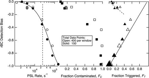
The value of these laboratory tests is in evaluating changes in measured SP2 rBC concentration due to independent changes in non-rBC particle loads and triggering parameters. Figure 2 shows results obtained with the standard SP2 setup: primary trigger from the scatter channel (DC coupled), with rBC-containing particles generating signal on the secondary trigger channel. This data was obtained with rBC concentrations of ∼500 rBC particles cm⁻³, i.e., a detection rate of ∼1000 s⁻¹. PSL particles were used for the scattering particles, with two different window lengths (i.e., total data points of 150 (solid markers, with 75 pre-trigger points) and 400 (empty markers, with 200 pre-trigger points)). By ramping up the rate of PSLs crossing the SP2 laser, the bias associated with trigger deadtime became more and more significant with higher loadings. The left-most panel shows bias magnitude increased as an exponential (fit) to nearly −1 (i.e., no detection of rBC-containing particles) as the scatter rate increased. At a PSL rate of ∼25,000 s⁻¹ (the nominal upper range of the SP2 specified by the manufacturer), the bias was ∼−40%. At the highest concentration/most severe bias, the PSL concentration was large enough to effectively disable triggering entirely for both channels, consistent with paralyzable deadtime effects for this SP2 configuration resulting from near-continuously co-incident PSLs holding the scatter signal above the threshold value. In the middle panel, it is clear that some information relevant to the excessively high particle rate was being recorded: F_C increased as bias became more and more important (middle panel). However, the relationship between F_C and bias was non-linear. Finally, the relationship between bias and F_T (right panel) was multi-valued, as the paralyzable effects of sustained high signals on the trigger channel increasingly disabled triggering and led to decreasing F_T with increasing scatter rate (as represented by the increasing marker size) even as bias magnitude increased, with almost no data saved at scattering rates of 150,000 s⁻¹. The dependence of these results on the length of each window and the pre-trigger length was very weak as paralyzable effects independent of pre-trigger length dominated deadtime. This particular setup of the SP2 is very sensitive to paralyzable deadtime under heavy particle loads because each particle raises the scatter signal over threshold for a fixed amount of time (depending on particle size and speed through the laser), and increasing particle rates increases the probability that the signal is sustained over threshold for extended periods past the point each scan for triggers begins.

Figure 2. Trigger bias measured with rBC particles externally mixed with mono-disperse rBC-free polystyrene latex (PSL) particles using the standard SP2 configuration (DC-coupled scatter signal as primary trigger channel). Empty/solid markers are for measurements with 400 or 150 points per detection respectively. Left: Bias plotted against the rate of PSLs crossing the SP2 laser. An exponential fit is shown with the solid line. The vertical dashed line shows the nominal maximum particle rate identified by the manufacturer. Center; Bias plotted against the fraction showing evidence of excessively high particle rates (as per text). Right: Bias plotted against the average fraction of buffer-time associated with triggered windows. In this plot, markers are scaled with PSL rate (between 1000 and 150,000 s⁻¹), with larger sizes corresponding to higher rates to show that the triggered fraction decreases at the largest biases/particle rates. The straight line shows the largest magnitude bias possible for a given fraction triggered, and the dashed line is the theoretical result from Equation (3)(3) $${\mathit{B}}_{\text{rel}}=-\left({\mathit{P}}_{\text{PT}}/\mathit{T}\_\mathit{P}\right)*{\mathit{F}}_{\mathit{T}}$$(3) .

SP2 deadtime sensitivity to high particle rates can be greatly reduced by reducing the probability of sustained signals. The most obvious ways to do this are by reducing sample flow and/or diluting the sample air. However, SP2 configuration choices are also important in affecting deadtime. A higher threshold value reduces the fraction of particles capable of triggering a detection and also reduces the time that a single particle causes the signal to stay above that threshold (although it would not change the calculation of F_C for the saved data). Using the position-sensitive detector to provide the primary channel of triggering is another way to accomplish this. This is effective because as a particle crosses the laser, the position sensitive detector produces both positive and negative signals, depending on the location of the particle. The negative signal contributes to bringing any threshold exceedance to an end, reducing paralyzable deadtime. Another route to reducing extended high signals is to use an AC-coupled scattering signal. AC coupling brings the signal average to the level of ground (zero potential). High particle rates lead to significant periods with non-background signal, so with the average held to zero, the result is a shift in the minimum signal (i.e., the baseline or background signal on the channel) to negative values. This, then, effectively increases the signal required to activate a triggered event (without the threshold being changed) with the benefits to deadtime that were just described. For example, imagine very few particles are transiting the laser. The AC coupling holds the background scatter signal to ∼0 volts. Now, imagine that particles enter the laser often enough that half the time there is no signal, and half the time—when a particle is in the laser—the signal is 1 V. The AC coupling brings the average to 0 V, so the background signal will be recorded as −0.5 V, and the particle signals will show up as 0.5 V. Each particle still generates a 1 V signal, but now it is referenced to a lower background level. Note that the position sensitive detector removes most background offsets due to the uniform illumination of both detection elements, and hence does not benefit from AC coupling in the same way that the scatter detector does. AC coupling the position-sensitive detector can still lead to baseline changes with particle loading as the positive and negative lobes produced by the position sensitive detector when properly set up (cross-over point at approximately the first ¼ of the laser) are different sizes. We generally use the position-sensitive detector in an AC-coupled mode.

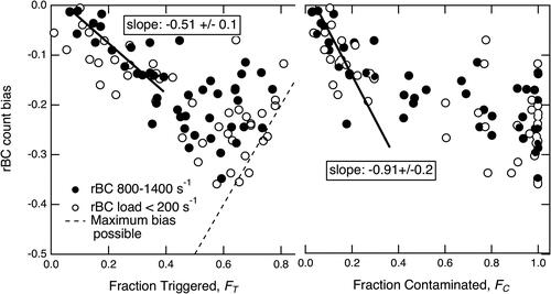
Figure 3 shows the improved range of bias observed with the primary trigger on either an AC-coupled scatter or position-sensitive channel for PSL scattering particles. The figure incorporates tests from many different configurations for sampling. The graph shows detection bias due to the primary triggering plotted against either F_T or F_C. The markers separate tests depending on the concentration of rBC used. Lower concentrations of rBC led to higher statistical uncertainties in calculating the bias, and hence show both larger scatter at most points along the abscissa and a larger magnitude bias at lower total concentrations (assumed due to the effect of statistical noise in the denominator of Equation (4)(4) $$B\mathrm{}=\mathrm{}\left(R_{PT}-R_{\mathit{Corr}}\right)/R_{\mathit{Corr}}$$(4) ). The left plot arranges the bias in terms of increasing F_T, with a fairly compact linear dependence at low to moderate F_T. On the right side, bias is plotted against F_C, with a less linear and compact dependence, suggesting that F_C is likely more useful in a qualitative rather than quantitative sense. The behavior of bias at low F_T and F_C is notable (i.e., at relatively low particle rates), because it was quite consistent with the non-paralyzable theory in all of the testing done for this study, with PSLs and polydisperse scattering aerosol, for all window lengths, trigger sources, and instrument setups (with pre-trigger points/total points held at ∼0.5). In this regime F_T and F_C can be used to constrain bias from the TA, and, in cases of need, may be suitable for removing some systematic bias. The results indicate that for F_C and F_T up to 0.3 the DC-coupled results were consistent with those shown here for AC coupling, and for the theoretical expectations (−0.5 slope for bias/F_T). Above those fractions, DC-coupled bias magnitude (Figure 2) grows more quickly than that of AC coupled or position-sensitive triggered configurations, as well as the theoretical estimate provided in Equations (1)(1) $$B_{\mathit{rel}}=\mathrm{}-R_S*\tau$$(1) and (3)(3) $${\mathit{B}}_{\text{rel}}=-\left({\mathit{P}}_{\text{PT}}/\mathit{T}\_\mathit{P}\right)*{\mathit{F}}_{\mathit{T}}$$(3) . AC-coupled and position-sensitive detector triggered bias can be even less than predicted by Equations (1)(1) $$B_{\mathit{rel}}=\mathrm{}-R_S*\tau$$(1) and (3)(3) $${\mathit{B}}_{\text{rel}}=-\left({\mathit{P}}_{\text{PT}}/\mathit{T}\_\mathit{P}\right)*{\mathit{F}}_{\mathit{T}}$$(3) or expected from paralyzable deadtime. This last is seen by the bias values in Figure 3 for F_T >∼0.5 that lie above the extrapolation of the linear fit at lower F_T, and is a consequence of the increasing probability of writing unscanned data to disk at high particle rates.

Figure 3. Bias in SP2 records of rBC particles plotted against (left) the fraction of the buffer associated with triggered windows and (right) the fraction of written windows that showed evidence of additional particle transects during the start of the window. Empty circles are for tests with relatively low rBC concentrations, and thus subject to larger relative statistical uncertainty. Filled circles were measured with high rBC concentrations and lower statistical uncertainty. The dashed line is the largest magnitude bias possible assuming that 100% of scanned windows can be associated with valid detection of an incandescent rBC-containing particle. The fits were only to high-rBC data. The fit on the left was to data <0.4 F_T and had an R² = 0.74. The fit on the right was to FC < 0.2 and had an R² of 0.6.

Choices of triggering parameters for a given scattering particle rate and rBC aerosol load can change bias with both F_T and F_C, especially at very high rates. We focus on the importance of individual factors here:

1. Window length: total data points with a fixed fraction of pre-trigger points:

   Figure 4 shows that the length of each window is important for influencing SP2 sensitivity to trigger bias, and should be minimized in conjunction with pre-trigger points for detection rates <∼10,000 s⁻¹ consistent with other constraints such as LEO-fitting window length requirements. These results are only pulled out for the case of an AC-coupled primary trigger, and for the extrema window lengths tested (150 points and 400 points), but the trends discussed here are quite consistent as a function of length in the results not shown. The shorter windows, with correspondingly shorter pre-trigger point lengths, result in lower bias at all scattering rates below ∼10,000 s⁻¹, merely due to the scaling of bias as shown in Equation (1)(1) $$B_{\mathit{rel}}=\mathrm{}-R_S*\tau$$(1) . However, at higher particle rates, longer windows performed better than shorter for the same rate. We hypothesize that this occurs because under extremely high loadings, paralyzable effects generate delays until triggering is re-enabled. With smaller windows, these delays occur more frequently than for longer windows. The result is that longer windows generate larger F_T than the shorter windows, thereby limiting the bias in BC. This is clear on the right panel for the same data (i.e., points with the same bias values in different panels are from the same test runs), where F_T extends to larger values with the longer windows and is associated with less bias for that reason. Up to F_T ∼ 0.4 the observed biases approximately match theory (Equation (3)(3) $${\mathit{B}}_{\text{rel}}=-\left({\mathit{P}}_{\text{PT}}/\mathit{T}\_\mathit{P}\right)*{\mathit{F}}_{\mathit{T}}$$(3) ) for low rates of particle coincidence. For the shorter windows, this match continues to higher F_T of ∼0.6. However, a smaller magnitude bias is observed for F_T greater than ∼0.4 for the longer-window results, where bias was capped at near −0.2 due to the reduction in bias from predictions when unscanned data is written to disk.

2. Primary trigger Source and AC/DC coupling:

   Trigger source can have an important impact on bias at very high particle rates, however, no clear differences between the different trigger sources were obvious in our tests for particle rates up to ∼8,000 s⁻¹. Above this rate, the DC-coupled scatter channel primary trigger should be avoided. For the AC-coupled channels, no significant difference in performance between the position-sensitive detector and the scatter detector was observed.

3. With and without skipping of scattering particles:

   Using skipping for primary-trigger only particles does not affect trigger bias on the secondary trigger, but does affect duty cycle (improved duty cycle occurs with skipping because the computer spends less time writing to disk) and reduces storage requirements. Note that if an incandescent signal would exceed that channel’s threshold at any point in a window, it would not be subject to consideration as a scatter-only detection.

4. On rBC concentration at fairly low concentrations:

   Testing was done at ∼500 and ∼1000 rBC particle s⁻¹ rates. No clear dependence of bias in this range was observed. At very high rBC concentrations, the same triggering algorithm problems explored for the scatter channel become relevant on the incandescent trigger channel; in that case the analyses explored here might be appropriate, but would need to be evaluated in a different way because the trigger could not simply be turned off and on to differentiate correct and potentially biased sampling. Analysis treatments for multiple incandescent peaks occurring in individual windows would likely need to be included. At such high rates of incandescent particle, the probability of physical problems (e.g., Zanatta et al. 2021) with detection increases.

5. With either mono-disperse PSLS or polydisperse scattering particles:

   A series of tests with both position-sensitive and a/c coupled scatter channel as triggering channel were conducted with a polydisperse aerosol generated by nebulizing diluted synthetic sea water. The bias observed was consistent with that measured with the monodisperse PSL tests.

Figure 4. Exploring the impact of window length on bias. This data selected only from cases of: PSL scattering particles with AC-coupled triggering for the two extreme window lengths (150 and 400 points). Markers are sized (large = long) with window length. Left: bias plotted against scatter particle rate. Right: bias plotted against the fraction triggered, which is itself a function of both particle rate and window length. The dashed line is the simple theoretical estimate of Equation (3)(3) $${\mathit{B}}_{\text{rel}}=-\left({\mathit{P}}_{\text{PT}}/\mathit{T}\_\mathit{P}\right)*{\mathit{F}}_{\mathit{T}}$$(3) .

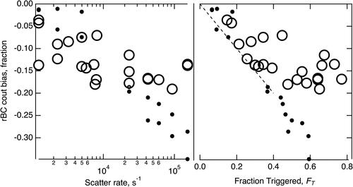
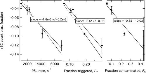
4.1. Bias at lower scatter particle rates

Of relevance to most common sampling situations with the SP2 in ambient conditions is the bias possible at the low end of scatter particle rates explored here. To address these conditions adequately in an experimental sense, statistically robust measurements of bias were conducted under a single parameter setup quite close to typical: 200 total data points with 100 pre-trigger points, primary triggering off the position-sensitive channel. For each data point, up to 10 measurements of the change of rBC rate with enabling/disabling of the primary trigger were made. To avoid bias from slow drifts in rBC concentrations from the nebulizer, bias measurements were made alternating enabling/disability or disabling/enabling in individual measurements. Average bias, F_C, and F_T were calculated with standard errors (i.e., the standard deviation divided by the square root of the number of observations less one). The results are shown in Figure 5, which shows linear dependences of bias on the rate of scattering particles, the fraction contaminated, and the fraction triggered. Comparison to Figure 3 reveals good agreement in the dependence (i.e., slope) of the bias on fraction triggered to the wider results and to the theoretical results in Equations (1)(1) $$B_{\mathit{rel}}=\mathrm{}-R_S*\tau$$(1) and (3)(3) $${\mathit{B}}_{\text{rel}}=-\left({\mathit{P}}_{\text{PT}}/\mathit{T}\_\mathit{P}\right)*{\mathit{F}}_{\mathit{T}}$$(3) (although this theory likely slightly over estimates bias at low but increasing detection rates). However, the relationship between the observed bias and the fraction contaminated is not consistent between these measurements (Figure 5, with a slope of −0.25) and those covering a much wider range of particle rate (Figure 3, with a slope of −0.91). For this reason, we identify the fraction triggered as more valuable for estimating possible bias, with the fraction contaminated being helpful for checking for the possibility of paralyzable effects when the DC coupled scattering detector is used as the primary trigger.

Figure 5. Relatively low-rate bias measured for 200 total data points, 100 pre-trigger points, position-sensitive detector providing primary scattering triggering. The solid lines are least-square fits to the data; the dashed lines are theoretical predictions based on Equations (1)(1) $$B_{\mathit{rel}}=\mathrm{}-R_S*\tau$$(1) and (3)(3) $${\mathit{B}}_{\text{rel}}=-\left({\mathit{P}}_{\text{PT}}/\mathit{T}\_\mathit{P}\right)*{\mathit{F}}_{\mathit{T}}$$(3) of the text.

5. Conclusion and recommendations

SP2 triggering algorithm bias should be considered in all measurements for which rBC absolute concentration is critical. Even under quite reasonable total particle rates (∼2000 s⁻¹) and typical choices of operational parameters, bias is detectable (∼4% low) if still lower than total SP2 uncertainty. In this range of particle rate, where particle co-incidence is rare, the simple model provided by Equations (1)(1) $$B_{\mathit{rel}}=\mathrm{}-R_S*\tau$$(1) and (3)(3) $${\mathit{B}}_{\text{rel}}=-\left({\mathit{P}}_{\text{PT}}/\mathit{T}\_\mathit{P}\right)*{\mathit{F}}_{\mathit{T}}$$(3) may be used with high confidence to assess bias (even for an aerosol dominated by rBC-containing particles). At higher rates, bias increases in magnitude. At the highest SP2 operational particle detection rate identified by the manufacturer (25,000 s⁻¹), low bias was 40% in the instrument’s typical configuration. Under extreme loadings and even higher rates, the bias can reach ∼100% for this “standard” SP2 configuration, or was capped at ∼−30% when scattering particles were triggered from the position sensitive detector.

Significant triggering bias occurs when particles cross the SP2 laser in very quick succession and/or simultaneously. These types of events leave two useful “signatures” in the stored data: the fraction of particles that show evidence of two additional particles transiting the laser shortly before them (“fraction contaminated,” F_C), and the fraction of sample time that was associated with trigger events (“fraction triggered,” F_T). These two measured parameters can be used to constrain, and in some cases, correct, the bias.

For an aerosol measurement at a given concentration, a number of SP2 configuration parameters need to be thoughtfully chosen with consideration of triggering bias. Based on the empirical laboratory results shown here, a first recommendation is that total trigger rate (a simple parameter to calculate, see Equation (2)(2) $${\mathit{F}}_{\mathit{T}}=({\mathit{N}}_{\mathit{S}}*\mathit{S}\_\mathit{S}+{\mathit{}\mathit{N}}_{\mathit{I}})*{\mathit{P}}_{\mathit{w}}*\left({\mathit{t}}_{\mathit{b}}\right)/{\mathit{T}}_{\mathit{B}}$$(2) ) be included as a basic data analysis parameter for consideration of bias potential, and automated flagging of data with high (as defined by the user) particle rate be used to ensure that bias is considered for any absolute rBC measurements. In cases where bias may or may not be significant, analysis of stored data for F_T and F_C can be used to constrain the magnitude of trigger bias with reasonable confidence. Specifically, with FC < 0.4, and F_T below ∼0.3, bias appears only weakly dependent on instrument operational parameters, and is quite compactly related to F_T as per Equation (3)(3) $${\mathit{B}}_{\text{rel}}=-\left({\mathit{P}}_{\text{PT}}/\mathit{T}\_\mathit{P}\right)*{\mathit{F}}_{\mathit{T}}$$(3) . We suggest 10% as a minimum additional uncertainty when correcting bias in this range. At F_T > ∼0.4 trigger bias varies more strongly with instrument parameters, and F_T alone can only be used to constrain maximum bias as suggested by Figure 3.

We recommend careful inspection of raw data to ensure correct sampling by the SP2 and analysis of recorded data. In laboratory conditions, changing SP2 measurement parameters and inspecting the resulting data to address bias (and other detection issues) is usually possible. For ambient sampling, any prediction of anticipated conditions (for example if sampling fresh wildfire plumes!) can be used to anticipate deadtime bias problems in advance of sampling. Trigger bias resulting from high scatter particle rates can be directly measured as was done here (given sufficient aerosol stability), even in otherwise unknown samples—this would be the most direct path to constraining the impact on the rBC measurement under stable conditions.

We recommend the following approaches to reducing the susceptibility of the SP2 rBC measurements to deadtime bias, depending on sampling needs determined by the user:

1. Disable triggering on non-rBC-containing particles by setting the threshold on the scatter or position-sensitive channel above the maximum value detected by the high-speed analog-to-digital converter of the SP2. For example, on a 5MS/s system, the digitizer maximum is 2047 counts; setting the primary threshold to e.g., 2200 disables all triggering on that channel, while still allowing the secondary channel to trigger off of incandescent signals. In this way, only particles generating signals on the incandescent channels will be recorded, and likelihood for bias will generally be greatly reduced so long as rBC concentrations are reasonable. Similarly, raising the appropriate threshold to reduce triggering rates from scatter particles will generally provide some benefit in terms of deadtimes. Note that high rates of rBC particles can also generate bias, but this situation was not dealt with in this manuscript. To use techniques such as developed here to address this, we would suggest using both the primary and secondary channel of triggering on the same incandescent channel, but with different threshold values and coupled with enabling/disabling the trigger with the lower threshold; or by comparing concentrations sampled at different sample flow rates.

2. AC-couple the scattering detector if using it for triggering on purely-scattering particles. Although this makes significant improvements in bias under extreme loads, as it helps to “break” the paralyzable deadtime effect, it does not improve biases at relatively low elevated trigger rates. We believe that using the position-sensitive detector for triggering makes better sense, as its behavior under heavy loads will be less dependent on the size distribution of the sample aerosol, and it provides triggers near a fixed position in the laser.

3. For scatter-particle detection rates up to ∼10,000/s, reduce the size of each trigger window if possible, with correspondingly shortened pre-trigger lengths. If only interested in recording incandescent signals from rBC particles, the windows can be made quite short after the scattering or position sensitive trigger is disabled, with shorter pre-trigger points than ½ the window length, reducing deadtime per trigger. As the leading edge of each incandescent peak is usually very steep, a pre-trigger of only 15 points with a 100-point window is generally reasonable starting point for recording only rBC incandescent information. For data products using LEO fitting or examination of scattering signals, a longer window and pre-trigger are both helpful for improving fit quality and necessary to capture scattering before incandescence begins. For LEO fitting, scattering particles should be saved to provide engineering data so both triggers are needed, and pre-trigger length must be maintained as well. It follows that LEO fit data-products will be more sensitive to bias and measurement artifacts from near co-incident particles than mere rBC concentrations. For scatter particle rates >10,000/s, our findings indicate that the reverse—longer windows—will be more successful in reducing deadtime.

4. Reduce the rate of sample flow into the SP2 so that a given concentration will translate to lower particle detection rates. This will also extend the time necessary to evaluate the rBC concentration and size distribution, and may cause problems due to increased particle transmission losses and flow calibration errors. Hence, we do not recommend extremely slow flows (<0.5 cm³ s⁻¹ without careful testing and calibration).

5. Dilute the sample. This will extend the time necessary to evaluate the rBC concentration and size distribution, and may cause problems associated with physical effects of dilution, dilution factor uncertainty, and increased particle transmission losses.

As always when making SP2 measurements of unusual aerosols, inspection of raw data and consideration of the broad variety of factors affecting the reliability of the data is a must.

Additional information

Funding

This work was carried out with partial support from the NASA Upper Atmosphere Composition Program and the NOAA Earth’s Radiation Budget Program.

References

- Cross, E. S., T. B. Onasch, A. Ahern, W. Wrobel, J. G. Slowik, J. Olfert, D. A. Lack, P. Massoli, C. D. Cappa, J. P. Schwarz, et al. 2010. Soot particle studies—instrument inter-comparison—project overview. Aerosol. Sci. Technol. 44 (8):592–611. doi:10.1080/02786826.2010.482113.
- Evans, R. D. 1955. The atomic nucleus. New York: McGraw-Hill.
- Feller, W. 1948. On probability problems in the theory of counters. In R. Courant anniversary volume, studies and essays, 105–15. New York: Interscience.
- Gao, R. S., J. P. Schwarz, K. K. Kelly, D. W. Fahey, L. A. Watts, T. L. Thompson, J. R. Spackman, J. G. Slowik, E. S. Cross, J.-H. Han, et al. 2007. A novel method for estimating light-scattering properties of soot aerosols using a modified single-particle soot photometer. Aerosol. Sci. Technol. 41 (2):125–35. doi:10.1080/02786820601118398.
- Katich, J. M., A. E. Perring, and J. P. Schwarz. 2017. Optimized detection of particulates from liquid samples in the aerosol phase: Focus on black carbon. Aerosol Sci. Technol. 51 (5):543–553.
- Laborde, M., P. Mertes, P. Zieger, J. Dommen, U. Baltensperger, and M. Gysel. 2012. Sensitivity of the Single Particle Soot Photometer to different black carbon types. Atmos. Meas. Tech. 5 (5):1031–43. doi:10.5194/amt-5-1031-2012.
- Schwarz, J. P., J. R. Spackman, R. S. Gao, A. E. Perring, E. Cross, T. B. Onasch, A. Ahern, W. Wrobel, P. Davidovits, J. Olfert, et al. 2010. The detection efficiency of the single particle soot photometer. Aerosol. Sci. Technol. 44 (8):612–28. doi:10.1080/02786826.2010.481298.
- Slowik, J. G., E. S. Cross, J.-H. H. Han, P. Davidovits, T. B. Onasch, J. T. Jayne, L. R. Williams, M. R. Canagaratna, D. R. Worsnop, R. K. Chakrabarty, et al. 2007. An inter-comparison of instruments measuring black carbon content of soot particles. Aerosol. Sci. Technol. 41 (3):295–314. doi:10.1080/02786820701197078.
- Zanatta, M., A. Herber, Z. Jurányi, O. Eppers, J. Schneider, and J. P. Schwarz. 2021. Technical note: Sea salt interference with black carbon quantification in snow samples using the single particle soot photometer. Atmos. Chem. Phys. 21 (12):9329–42. doi:10.5194/acp-21-9329-2021.