Molecular composition and gas-particle partitioning of indoor cooking aerosol: Insights from a FIGAERO-CIMS and kinetic aerosol modeling

Abstract

Organic aerosol emitted from cooking is a major concern for indoor air quality. During the House Observations of Microbial and Environmental Chemistry (HOMEChem) campaign, we simulated cooking, cleaning and occupancy activities in a realistic residential setting and measured resulting gas- and particle-phase emissions using a High-Resolution Time-of-Flight Chemical Ionization Mass Spectrometer with a Filter Inlet for Gases and Aerosols (FIGAERO-HR-ToF-CIMS). We identified ∼480 molecular formulas for compounds emitted on cooking-centered days and attributed them to potential sources including cooking, commercial, personal care products, and occupancy. Compounds with molecular formulas containing carbon, hydrogen, and oxygen atoms only (CHO group) composed most of the CIMS-measured molar fraction at 74-85%, with nitrogen-containing molecular formulas (CHNO group) being the second largest contributor (12-19%). We investigated the volatility of identified species based on FIGAERO-CIMS data in three ways: (1)(1) $$\mathit{Particle} \mathit{signal} \mathit{\left[}\frac{ions}{volume}\right]=\frac{\mathit{Integrated} \mathit{particle} \mathit{signal} \left[\mathit{ions}\right]}{Particle collection period \mathit{\left[}min\right]\mathit{\times }Particle collection rate \left[{\displaystyle \frac{L}{min}}\right]}$$(1) using the maximum desorption temperature from one-dimensional thermograms, T_max, (2)(2) $$\mathit{Gas} \mathit{signal}\mathit{ }\mathit{\left[}\frac{\mathit{i}\mathit{o}\mathit{n}\mathit{s}}{\mathit{s}\mathit{e}\mathit{c}}\right]=\frac{\mathit{Av}g\mathit{.} \mathit{gas} \mathit{signal} \left[\frac{\mathit{ions}}{\mathit{sec}}\right]}{\mathit{CIMS} \mathit{sampling} \mathit{rate} \left[\frac{L}{sec}\right]}$$(2) calculating gas-particle partitioning, F_p, (3)(3) $$F_p=\frac{\mathit{Particle} \mathit{signal} \left[\frac{\mathit{ions}}{\mathit{vol}}\right]}{\mathit{Gas} \mathit{signal} \left[\frac{\mathit{ions}}{\mathit{vol}}\right]+\mathit{Particle} \mathit{signal} \left[\frac{\mathit{ions}}{\mathit{vol}}\right]}$$(3) using a molecular corridor parameterization to estimate saturation concentrations based on molecular formulas. We used the kinetic multi-layer model of gas-particle interactions in aerosols and clouds (KM-GAP) to calculate equilibration timescales and found that under sampling conditions (T = 323 K), it can take up to 14 seconds for equilibrium conditions to be met, whereas sampling residence times are approximately 3 seconds. The chemical diversity and wide range of volatilities of species sampled during cooking-centered events highlight the importance of understanding aerosol emissions and partitioning in indoor spaces where people spend most of their time.

EDITOR:

• Jonathan P. Reid

1. Introduction

Small airborne particles are known to have deleterious impacts on human health, including increased risk of mortality, cardiovascular diseases, impaired lung function, and strokes (Burnett et al. 2018; Nel 2005; Anderson, Thundiyil, and Stolbach 2012; Pope and Dockery 2006). In the United States and in most of the developed world, people spend an average of 90% of their time indoors, 70% of that within residences (Klepeis et al. 2001), where pollutant levels can be orders of magnitude higher than outdoors (Klein et al. 2016). It is therefore probable that most human exposure to air pollutants occurs within the indoor environment, specifically within residential homes. Cooking, one of the most common activities carried out in a household, has been recognized as a major contributor to elevated particulate matter (PM) concentrations in indoor air (Abdullahi, Delgado-Saborit, and Harrison 2013; Nasir and Colbeck 2013; Huboyo, Tohno, and Cao 2011; Wan et al. 2011) and outdoor air in urban areas (Elser et al. 2016; Crippa et al. 2013; Mohr et al. 2012; Slowik et al. 2010; Allan et al. 2009). In most developed countries, cooking is considered the main source of primary PM in the indoor environment (Wallace 2006).

Previous studies have primarily used Aerosol Mass Spectrometers (AMS, Aerodyne Research Inc.) (DeCarlo et al. 2006; Drewnick et al. 2005; Jayne et al. 2000) or offline particle analysis for chemical characterization of cooking aerosol. High resolution aerosol mass spectrometers (HR-AMS) were used to measure emissions from meat cooking on a propane grill (Mohr et al. 2009), from seed oils heated in a metallic container (Allan et al. 2009), and from cooking oils that were photo-oxidized in a smog chamber (Liu et al. 2018). A limitation of aerosol mass spectrometers is their use of flash vaporization (at 600 °C) followed by 70 eV ionization to enable aerosol detection, which leads to fragmentation of analytes and hinders determination of the original molecular composition of sampled species. Off-line particle analysis was used to study the chemical composition of PM_2.5 emissions from four restaurants in China (Li, Wu, et al. 2021), to measure emissions from charbroiling and grilling of meats at a test kitchen (Mcdonald et al. 2003), and to measure polycyclic aromatic hydrocarbons and aldehydes released during beefsteak frying in a model kitchen (Sjaastad, Jørgensen, and Svendsen 2010). Limitations of offline techniques include their relatively low time resolution and their propensity for artifacts, such as those associated with the reaction of trace gases with the particles on the filter, or with the filter itself (Abdullahi, Delgado-Saborit, and Harrison 2013).

In this work we measured gas- and particle-phase emissions from cooking using a High-Resolution Time of Flight Chemical Ionization Mass Spectrometer (HR-ToF-CIMS) coupled with a Filter Inlet for Gases and Aerosols (FIGAERO). The FIGAERO-HR-ToF-CIMS (hereafter referred to as FIGAERO-CIMS) utilizes soft ionization to provide information on molecular chemical composition and volatility of measured species. It enables near-simultaneous sampling of the gas and particle phases, at a time resolution of 1 Hz or higher for the gas phase, and minutes to a few hours for the particle phase. The FIGAERO-CIMS has the advantage of measuring molecular composition while avoiding filter-associated artifacts and providing information on volatility through the quasi-online measurements of the gas and particle phases. A recent study used the FIGAERO-CIMS in combination with a HR-AMS to study cooking aerosol from different meals in a controlled laboratory setting (Reyes-Villegas et al. 2018).

To determine exposure and health impacts of pollutants, both their chemical composition and partitioning between the gas and particle phases need to be characterized. The bio-accessibility of PM-associated pollutants and therefore their impact on human health varies depending on particle size and partitioning of compounds between the gas and particle phases (Nováková et al. 2020). Gas-particle partitioning is determined in part by a compound’s vapor pressure or volatility (Pankow 1994, 2001). Previous studies have attempted to constrain organic aerosol (OA) volatility by thermal evaporation (thermodenuders), isothermal dilution, or a combination of both methods (Voliotis et al. 2021; Cain, Karnezi, and Pandis 2020; Louvaris et al. 2017; Karnezi, Riipinen, and Pandis 2014; Riipinen et al. 2010; Grieshop et al. 2009; Huffman et al. 2008, 2009). The FIGAERO-CIMS can provide an advantage over previous volatility measurement techniques in that it measures the contribution of individual compounds in the gas and particle phases in near-real time, allowing for a direct calculation of compound-specific partitioning values (Lopez-Hilfiker et al. 2014, 2015).

In this work, we characterized aerosol generated from cooking during the House Observations of Microbial and Environmental Chemistry (HOMEChem) experiments, which simulated cooking activities in a realistic kitchen and home setting. The campaign was a field perturbation experiment where indoor activities including cooking were carefully designed and implemented, and where external conditions such as fluctuations in meteorology and building parameters were allowed to influence sources and sinks in indoor air (Farmer et al. 2019). A variety of instrumentation provided insights into the air pollutant mixture released from cooking. Measurements of particle size distribution showed PM_2.5 concentrations exceeding 250 μg m⁻³ during cooking activities (Patel et al. 2020; Boedicker et al. 2021). Measurements of semi-volatile compounds showed that volatility and partitioning phenomena were key factors influencing SVOC concentration variability indoors (Lunderberg et al. 2020). Films over indoor surfaces – likely formed during cooking activities – were found to act as a reservoir for gas-phase species during ventilation experiments (Wang et al. 2020), and organic films analyzed using offline AMS and offline Fourier Transform Ion Cyclotron Resonance Mass Spectrometry (FT-ICR-MS) contained material similar to cooking organic aerosol measured by an online AMS, albeit more oxidized and highly viscous (O’Brien et al. 2021). Over 200 particle-phase species (predominantly fatty acids, carbohydrates, phthalates) released from cooking or sorbed into cooking particles were identified in real-time using extractive electrospray ionization mass spectrometry (Brown et al. 2021). Low volatility siloxane emissions were observed during oven use identifying certain appliances as another source of emissions (Katz, Guo, et al. 2021). Measurements from a gas-phase chemical ionization mass spectrometer showed that elevated PM concentrations that occurred due to cooking activities had implications on indoor air quality not only during the cooking event itself, but also during later cleaning activities (Mattila et al. 2020).

To the best of our knowledge, the work presented here is the first to investigate emissions from scripted cooking experiments in a highly realistic home setting using a FIGAERO-CIMS instrument, with cleaning and occupancy activities occurring in parallel. The objectives of this study were to use a FIGAERO-CIMS to: (1)(1) $$\mathit{Particle} \mathit{signal} \mathit{\left[}\frac{ions}{volume}\right]=\frac{\mathit{Integrated} \mathit{particle} \mathit{signal} \left[\mathit{ions}\right]}{Particle collection period \mathit{\left[}min\right]\mathit{\times }Particle collection rate \left[{\displaystyle \frac{L}{min}}\right]}$$(1) identify compounds emitted from cooking-centered activities, (2)(2) $$\mathit{Gas} \mathit{signal}\mathit{ }\mathit{\left[}\frac{\mathit{i}\mathit{o}\mathit{n}\mathit{s}}{\mathit{s}\mathit{e}\mathit{c}}\right]=\frac{\mathit{Av}g\mathit{.} \mathit{gas} \mathit{signal} \left[\frac{\mathit{ions}}{\mathit{sec}}\right]}{\mathit{CIMS} \mathit{sampling} \mathit{rate} \left[\frac{L}{sec}\right]}$$(2) suggest possible sources for these compounds, (3)(3) $$F_p=\frac{\mathit{Particle} \mathit{signal} \left[\frac{\mathit{ions}}{\mathit{vol}}\right]}{\mathit{Gas} \mathit{signal} \left[\frac{\mathit{ions}}{\mathit{vol}}\right]+\mathit{Particle} \mathit{signal} \left[\frac{\mathit{ions}}{\mathit{vol}}\right]}$$(3) characterize the compounds’ gas-particle partitioning indoors and (4)(4) $$C_i^{*}=\frac{(1-F_p)}{F_p}\times C_{OA}$$(4) evaluate the equilibration timescales for partitioning of organic aerosol during cooking experiments.

2. Methodology

2.1. Campaign set-up

The House Observations of Microbial and Environmental Chemistry (HOMEChem) campaign was an indoor air measurement campaign conducted in June 2018 at the University of Texas Test House (UTest House). The UTest House is a 3-bedroom, 2-bathroom, premanufactured home located at the J. J. Pickle Research Campus in Austin, TX. It has a surface area of 111 m,² volume of 250 m,³ and heating ventilation and air conditioning (HVAC) systems which provided a constant outdoor air flow of ∼0.5 ACH (air changes per hour) for the duration of the campaign. A description of the test house floor plan and other campaign set-up details can be found in Farmer et al. (2019). Some instrumentation was located inside the UTest House, while most instruments (including the FIGAERO-CIMS used in this study) were in air-conditioned trailers beside the test house at an approximate distance of 5 meters. In this study, we measured gas- and particle- phase species using a FIGAERO-CIMS which had four separate inlets for indoor/outdoor switching and gas-/particle-phase sampling. We used 1/4" PFA tubing for the gas-phase inlets and 3/8" O.D. stainless steel tubing for the particle phase inlets. The indoor inlet lengths from the kitchen to the instrument were 8.4 m and the outdoor inlet lengths from the outdoor sampling point (top of trailer) to the instrument were 2.1 m. Flow rates through the inlets were ∼6 L min⁻¹ for the gas phase and ∼11 L min⁻¹ for the particle phase lines. This is equivalent to residence times of 1.5 and 2.7 seconds for indoor gas and particle sampling, respectively.

The campaign included activities of cooking, cleaning, and human occupancy. The focus of this study is cooking-centered days, specifically “Layered days” and “Thanksgiving days”. Layered days involved the preparation of breakfast (English breakfast), lunch (vegetable stir fry), and dinner (beef chili) with cleaning activities occurring throughout the day (e.g., wiping down counters with disinfectant wipes, mopping floors with various cleaning solutions). The Thanksgiving days involved preparation of various dishes including a Thanksgiving turkey, sweet potato casserole, roasted brussels sprouts, and mulled wine, also with intermittent cleaning activities. Both days included emissions from occupants who conducted the cooking and cleaning activities (Farmer et al. 2019). The subsequent analysis will focus mainly on cooking events during these days. We limit the analysis to experiment days in the second half of the HOMEChem campaign when FIGAERO-CIMS sensitivity was optimal.

2.2. Iodide FIGAERO-CIMS

The High-Resolution Time of Flight Chemical Ionization Mass Spectrometer (CIMS, Aerodyne Research) ran in iodide (I^-) mode which provides good sensitivity toward organic species that are slightly to highly oxidized, chlorinated (or halogenated) species, and nitrogenated species (Lee et al. 2014). Ultra-high purity nitrogen gas (UHP N₂) passed through a bubbler to humidify the reagent gas stream, then through a methyl iodide (CH₃I) permeation tube, and the resulting humidified reagent gas stream passed through a Po-210 source to generate I^- and (H₂O)I^- ions. The I^- and (H₂O)I^- ions encounter the gas-phase analyte (M) stream in the ion molecule reaction (IMR) region of the CIMS, forming M.I^- or M.I(H₂O)^- adducts. Deprotonation products of inorganic acids and small organic acids are also present (Lee et al. 2014), but for this study we focus only on I^- adducts. These adducts then transfer to the Time of Flight (ToF) chamber in the CIMS where their time of flight is determined, which is related to their mass-to-charge ratio (m/z).

The FIGAERO inlet on the CIMS enables particle-phase measurements. Briefly, we collected particles onto a 1.0 µm polytetrafluoroethylene (PTFE) filter (Pall Corporation) during online gas-phase measurements. The particle collection period varied from 20-60 min based on the organic aerosol loading conditions (C_OA) inside of the house. We standardized the particle collection start time to align with a start time at the top of the hour, which matched up with the start of the cooking events. The filter material and treatment sequence (e.g., temperature ramp-up rate) remained consistent for all experiments analyzed to ensure thermogram reproducibility. After the simultaneous particle collection and online gas-phase measurement period, the filter with deposited particles was moved via an actuator to align with the HR-ToF-CIMS inlet. During particle-phase measurement, heated UHP N₂ gas passed through the PTFE filter to volatilize the sampled particles. Particle desorption took place over 40 min during which no gas-phase measurements were taken. The desorption routine included 2 min of room temperature desorption, 18 min of a temperature ramp from 25-200 °C, 5 min of filter soaking at 200 °C, and 10 min of cooling back to 25 °C. The FIGAERO-CIMS provided hourly particle-phase measurements and, outside the aerosol desorption period, online (1 Hz) gas-phase measurements. A detailed description of the working mechanism of the FIGAERO-CIMS is presented by Lopez-Hilfiker et al. (2014).

2.3. Data analysis

We analyzed the FIGAERO-CIMS data using Tofware v2.5.11 (Tofwerk, AG) in Igor Pro v6.37 (Wavemetrics Inc.). The conversion of ion time-of-flight to mass-to-charge (m/z) was based on 3 calibrants: I^-, (H₂O)I^- and I₃^-. The exact m/z values were subsequently used to assign elemental formulas to detected analytes. We report ions consistent with iodide-adducts of closed-shell products in Table S2 and use these for subsequent analyses. Detection of radical species is unlikely considering the sampling line length. Although the FIGAERO-CIMS cannot resolve isomeric ions, a priori information about the emission source and activities facilitated ion assignment. For instance, oils used in cooking are more likely to release organics including fatty acids, while cleaning events that use bleach are likely to emit chlorine-containing compounds. We cross-referenced identified species with publicly available databases (e.g., Pubchem) whenever possible. We corrected the high-resolution time-series for background (see Section S1 in Supplement for more details) and normalized signals by the dominant reagent ion (I^-) to account for changes in instrument sensitivity. For each compound, we converted the gas- and particle-phase signals to counts per volume of air sampled as shown in Equations (1)(1) $$\mathit{Particle} \mathit{signal} \mathit{\left[}\frac{ions}{volume}\right]=\frac{\mathit{Integrated} \mathit{particle} \mathit{signal} \left[\mathit{ions}\right]}{Particle collection period \mathit{\left[}min\right]\mathit{\times }Particle collection rate \left[{\displaystyle \frac{L}{min}}\right]}$$(1) and (2)(2) $$\mathit{Gas} \mathit{signal}\mathit{ }\mathit{\left[}\frac{\mathit{i}\mathit{o}\mathit{n}\mathit{s}}{\mathit{s}\mathit{e}\mathit{c}}\right]=\frac{\mathit{Av}g\mathit{.} \mathit{gas} \mathit{signal} \left[\frac{\mathit{ions}}{\mathit{sec}}\right]}{\mathit{CIMS} \mathit{sampling} \mathit{rate} \left[\frac{L}{sec}\right]}$$(2) . We estimated gas-particle partitioning, F_p, as shown in Equation (3)(3) $$F_p=\frac{\mathit{Particle} \mathit{signal} \left[\frac{\mathit{ions}}{\mathit{vol}}\right]}{\mathit{Gas} \mathit{signal} \left[\frac{\mathit{ions}}{\mathit{vol}}\right]+\mathit{Particle} \mathit{signal} \left[\frac{\mathit{ions}}{\mathit{vol}}\right]}$$(3) from Stark et al. (2017). Equation (4)(4) $$C_i^{*}=\frac{(1-F_p)}{F_p}\times C_{OA}$$(4) enables calculation of saturation concentration from partitioning numbers and vice versa. Our analysis of F_p is limited to compounds exhibiting unimodal desorption behavior due to the complexity of separating two (or more) integrals in a multimodal desorption profile, and to limit the influence of fragmentation products. (1) $$\mathit{Particle} \mathit{signal} \mathit{\left[}\frac{ions}{volume}\right]=\frac{\mathit{Integrated} \mathit{particle} \mathit{signal} \left[\mathit{ions}\right]}{Particle collection period \mathit{\left[}min\right]\mathit{\times }Particle collection rate \left[{\displaystyle \frac{L}{min}}\right]}$$(1) (2) $$\mathit{Gas} \mathit{signal}\mathit{ }\mathit{\left[}\frac{\mathit{i}\mathit{o}\mathit{n}\mathit{s}}{\mathit{s}\mathit{e}\mathit{c}}\right]=\frac{\mathit{Av}g\mathit{.} \mathit{gas} \mathit{signal} \left[\frac{\mathit{ions}}{\mathit{sec}}\right]}{\mathit{CIMS} \mathit{sampling} \mathit{rate} \left[\frac{L}{sec}\right]}$$(2) (3) $$F_p=\frac{\mathit{Particle} \mathit{signal} \left[\frac{\mathit{ions}}{\mathit{vol}}\right]}{\mathit{Gas} \mathit{signal} \left[\frac{\mathit{ions}}{\mathit{vol}}\right]+\mathit{Particle} \mathit{signal} \left[\frac{\mathit{ions}}{\mathit{vol}}\right]}$$(3) (4) $$C_i^{*}=\frac{(1-F_p)}{F_p}\times C_{OA}$$(4)

One-dimensional thermograms, which are plots of desorption signal versus temperature, provide insight into the volatility of individual species. The use of T_max – the temperature at which the highest signal is observed in a desorption thermogram – has been proposed as a method of inferring volatility from FIGAERO-CIMS data (Bannan et al. 2018; Schobesberger et al. 2018; Lopez-Hilfiker et al. 2014). We determined T_max for every compound from its one-dimensional thermogram. For compounds exhibiting multimodal behavior in their thermograms, we used the first (lowest) T_max value for subsequent analysis. Multimodal desorption behavior may indicate either a decomposition product from a parent ion, or presence of isomers with different vapor pressures (Buchholz et al. 2019; Wang and Hildebrandt Ruiz 2018; Stark et al. 2017; Lopez-Hilfiker et al. 2015). A limitation of this analysis is that some low-concentration compounds had broad thermograms, making it challenging to determine a distinct T_max. Additionally, T_max can depend on filter loading (Masoud and Hildebrandt Ruiz 2021; Huang et al. 2018; Wang and Hildebrandt Ruiz 2017), which introduces uncertainty when inferring vapor pressures from T_max.

We also used two-dimensional thermograms to visualize the volatility of the entire mass spectrum (Wang and Hildebrandt Ruiz 2018). Creating two-dimensional thermograms involves compiling one-dimensional plots of particle signal (normalized to its maximum value) versus desorption temperature at each m/z into a single 2 D plot where the vertical axis is the unit m/z, the horizontal axis is desorption temperature (°C), and the plot is colored by normalized signal intensity.

2.4. KM-GAP model setup

We used the kinetic multi-layer model of gas-particle interactions in aerosols and clouds (KM-GAP) to calculate equilibration timescales (τ_eq) in gas-particle partitioning and to simulate the partitioning number (F_p) for individual compounds with different saturation concentrations (C⁰) (Shiraiwa et al. 2012). The multiple model compartments and layers in KM-GAP include a gas phase, a near-surface gas phase, a sorption layer, a surface layer, and a number of bulk layers. The gas phase diffusion, adsorption/desorption, surface-bulk exchange, and bulk diffusion were treated as temperature-dependent (Li and Shiraiwa 2019). Table 1 shows the parameters and their values which were inputs to the model.

Table 1. Parameters and their values used in KM-GAP simulations for a specific cooking event.

Parameter (Unit)	Description	Values
Tg,org (K)	Tg of organic particles under dry conditions	276
RH (%)	Relative humidity	28
T (K)	Temperature	322.8 (average temperature during event) 298 (room temperature)
COA (μg m^−3)	Mass concentration of total organic aerosols	134 1000 (for sensitivity simulations)
C^0 (μg m^−3)	Saturation mass concentration of the partitioning compounds	varied over the range of 10^−2–10^6
η (Pa s)	Viscosity of organic particles	2.2 × 10^3 at measured RH and T 5.7 × 10^5 at measured RH and room T
Db (cm^2 s^−1)	Bulk diffusion coefficient	3 × 10^−12 at measured RH and T 1 × 10^−14 at measured RH and room T
αs,0	Surface accommodation coefficient on free-substrate	1

The particle phase state strongly affects gas-particle partitioning. The viscosity (η) of organic particles can be characterized by the glass transition temperature (T_g), at which the phase transition between amorphous solid and semi-solid states occurs (Koop et al. 2011). We predicted the T_g of a compound i with a single T_max (i.e., T_max for unimodal desorption behavior) using the parameterization of DeRieux et al. (2018): (6) $$T_{g,i}=(n_C^0 +ln\left(n_C\right))b_C+ln\left(n_H\right)b_H+ln\left(n_C\right)ln\left(n_H\right)b_{CH}+ln\left(n_O\right)b_O+ln\left(n_C\right)ln\left(n_O\right)b_{CO}$$(6) n_C, n_H, and n_O represent the number of carbon, hydrogen, and oxygen atoms, respectively. Values of the coefficients [$n_C^0,$ b_C, b_H, b_CH, b_O, and b_CO] are [12.13, 10.95, −41.82, 21.61, 118.96, −24.38] for CHO compounds. The analysis excluded compounds containing other heteroatoms (i.e., N or S). We estimated T_g of organic particles under dry conditions (T_g,org) using the Gordon-Taylor equation with the Gordon-Taylor constant (k_GT) of 1 (Dette et al. 2014), which resulted in a predicted T_g,org of 276 K (Table 1). We assumed that the relative mass concentration of each compound is proportional to its relative intensity in the mass spectrum.

The phase state of organic particles under humid conditions depends on the water content in particles (Mikhailov et al. 2009; Koop et al. 2011). To calculate the viscosity of organic-water mixtures, we used the effective hygroscopicity parameter (κ) – assumed to be 0.1 for cooking OA based on a previous study (Li et al. 2018) – to estimate the water content in organic particles (Petters and Kreidenweis 2007). We calculated T_g of organic-water mixtures (T_g,mix) using the Gordon-Taylor equation with k_GT of 2.5 (Koop et al. 2011; Zobrist et al. 2008). We then used T_g,mix to compute the temperature-dependence of viscosity using the Vogel-Tammann-Fulcher (VTF) equation, with the fragility parameter (D) assumed to be 10 based on our previous work (DeRieux et al. 2018). The viscosity calculated based on the average temperature measured during the simulated cooking event provides insight into the phase state of the cooking OA. Note that the estimated viscosity can be regarded as a lower bound as we excluded compounds with multimodal behavior (i.e., multiple T_max values) or nitrogen-containing compounds which may have high T_g. The Stokes–Einstein equation gives the value for the bulk diffusion coefficient D_b, and it was demonstrated to work well for organic molecules diffusing through materials with viscosity below ∼10³ Pa s (Chenyakin et al. 2017). We also computed the viscosity and D_b at room temperature to investigate the effect of viscosity on τ_eq. We investigated the effect of C⁰ on τ_eq by varying C⁰ from 10⁻² – 10⁶ μg m⁻³.

The measured average particle number size distribution (Figure S1) and the mass concentration of total organic aerosols during the simulated cooking event were inputs to the KM-GAP model. We did not consider particles with diameter < 20 nm. Their number concentrations decreased with time during cooking events (e.g., 14:05-14:25 shown in Figure S2), indicating that these small particles underwent coagulation, which was not considered in KM-GAP. To investigate the effect of C_OA on τ_eq, we ran sensitivity simulations at C_OA of 10³ μg m⁻³ by increasing the particle number in each particle size bin (Figures S3 and S4). A closed system was considered, in which condensation of compound i leads to a decrease in its gas-phase mass concentration and an increase in its particle-phase mass concentration.

Figure 1. "Signature" emissions observed during (a) layered day 4 (b) Thanksgiving day 2. The main cooking events occurred in the middle time period shown (i.e., beef chili at 16:05-16:25 and sweet potato casserole at 14:05-14:25). The bars are clustered, with signals for all three time periods starting at zero.

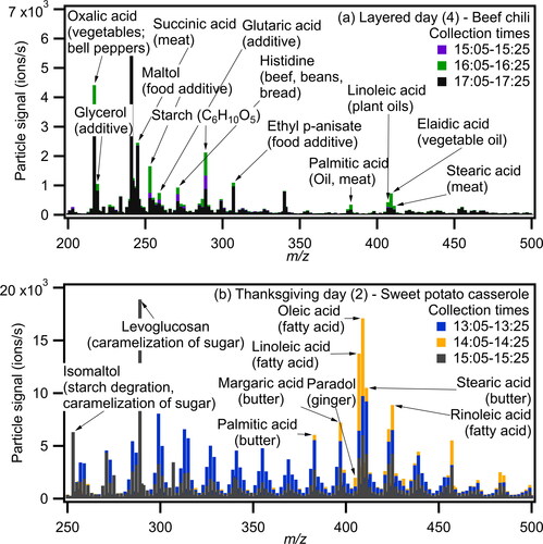
Figure 2. Distribution of measured particle-phase compounds by elemental groups: CHO, CHNO, CHClO, CHClNO, CHN, CHSO, CHNSO. The distributions are shown for (a) L3_VS: Layered day 3 – Vegetable stir fry 11:35-12:35, (b) L4_EB: Layered day 4 – English breakfast 9:05-9:25, (c) L4_VS: Layered day 4 – Vegetable stir fry 12:05-12:25, (d) L4_BC: Layered day 4 – Beef chili 16:05-16:25, (e) TG1: Thanksgiving day 1 – 14:30-15:30, (f) TG2: Thanksgiving day 2 – 14:05-14:25, (g) TG2_cat: Distribution by source category for Thanksgiving day 2 – 14:05-14:25. NO_x concentrations are shown on the top panel in units of ppb_v.

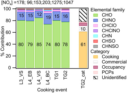
Figure 3. Aggregated signal separated by carbon and oxygen number for (a) CHO for L4_EB (b) CHNO for L4_EB (c) CHO for TG2 (14:05-14:25) (d) CHNO for TG2 (14:05-14:25). Labeled signals are for identified compounds with the highest abundance within each category.

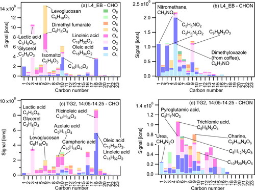
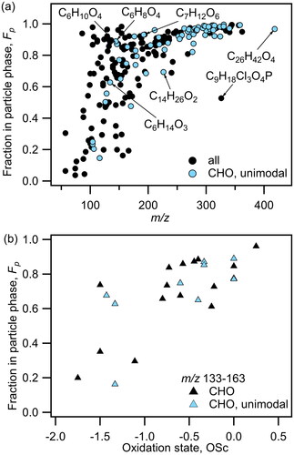
Figure 4. a) Fraction of HR-identified compounds in the particle phase versus molar mass (m/z) for TG2, particle collection period of 14:05-14:25. Compounds shown in black are all HR-identified compounds for this time-period. Compounds shown in blue are CHO-only unimodal compounds. (b) F_p of non-nitrogenated compounds in m/z region 133-163 from (a) versus their oxidation states (OSc).

The full equilibration timescale (τ_eq) is calculated when the following criterion is met, (7) $$\frac{\left|C_p\left(t\right)-C_p,eq\right|}{C_{p,0}-C_p,eq}<1\%$$(7) where C_p,0 and C_p,eq are the initial and equilibrium mass concentration of the partitioning compound in the particle phase, respectively.

These methods to estimate saturation mass concentration (C₀) and glass transition temperature (T_g) do not consider the effects of isomers. While C₀ and T_g are generally well characterized by molecular size and elemental composition (Murphy et al. 2011; Donahue et al. 2011), we acknowledge that molecular structure and functionality can also impact these properties (Koop et al. 2011). The FIGAERO-CIMS is unable to measure functionality or structure, which presents a limitation of this study.

3. Results and discussion

We present the results of various cooking events including a sequential stir fry, two Thanksgiving days, and three layered days (which included an English breakfast, stir fry lunch and chili dinner). Table S1 summarizes the cooking events discussed in this work and the analysis conducted for each event.

3.1. Molecular composition

Following the procedure outlined in Section 2.3, we identified 481 compounds in the gas and particle phases from the FIGAERO-CIMS spectra, 169 of which are compounds we attribute to cooking activities. Results are illustrated in Figures 1 and 2, and a list of all identified species and their presumed sources is provided in Table S2. We use the particle-phase mass spectra from the FIGAERO-CIMS to identify signature emissions, which we find to be consistent with the corresponding cooking events. When occupants prepared beef chili, we observed signature compounds including C₆H₉N₃O₂ which is the molecular formula of histidine, potentially released from beef and beans (Holeček 2020), and C₂H₂O₄ which is the molecular formula of oxalic acid, potentially released from bell peppers (Luning et al. 1995; as shown in Figure 1a which captures the period before, during and after the chili was cooked).

Figure 1b shows the particle phase mass spectra before, during and after a sweet potato casserole was cooked. We observed notable signals which include C₆H₆O₃, likely isomaltol, which is released from caramelization of sugar (Ito 1977), C₁₇H₂₆O₃, likely paradol, which is released from ginger (Shi et al. 2021), and several compounds associated with butter such as C₁₇H₃₄O₂ (potentially margaric acid), C₁₆H₃₂O₂ (potentially palmitic acid), and C₁₈H₃₆O₂ (potentially stearic acid) (Pădureţ 2021).

We group the identified molecular formulas into the following elemental groups: CHO (i.e., the group of compounds containing only C, H, and O atoms), CHNO, CHClO, CHNClO, CHSO, CHN, and CHNSO. Figure 2 summarizes the molar distribution of identified compounds in the particle phase based on elemental groups. The distribution is based on the integrated particle phase signal which is proportional to molar concentration, assuming uniform mass-dependent transmission efficiency and uniform sensitivity. For all reported cooking events, the CHO group has the highest contribution overall (∼74% to 85%), followed by CHNO (∼12% to 19%). The prevalence of the CHO group is consistent with most (I^- CIMS-detectible) cooking emissions being oxidized hydrocarbons such as fatty acids.

The nitrogen content in organic PM may relate to the composition of the food being cooked and/or the concentration of NO_x within the kitchen at the time of cooking. Comparing the elemental distribution of different cooking events on Layered Day 4 (English breakfast, vegetable stir-fry lunch and beef chili dinner, i.e., L4_EB, L4_VS, L4_BC panels respectively in Figure 2), we find that the CHNO group contribution varies from 11.9-18.8%. Indoor NO_x levels (associated with the gas stove pilot lights) were 95.5, 153 and 203 ppb_v for the breakfast, lunch, and dinner respectively (Farmer et al. 2019). Based on the ingredients being cooked (i.e., the meat and plant-based protein content in the food), we presume that the level of protein was highest for the chili dinner (which contained beef and beans), followed by the English breakfast (which contained sausage), followed by the vegetable stir fry (which included white rice and vegetables). The CHNO group contribution for the different meals followed the trend of the presumed nitrogen content of the food, not the trend of the NO_x concentration inside of the house, suggesting that food nitrogen content impacts the CHNO contribution to organic aerosol from cooking.

Given the continuous cooking activity that took place on the simulated Thanksgiving days (shown in panels TG1 and TG2 in Figure 2), we further studied the categorical distribution of observed compounds from Thanksgiving day 2 at 14:05-14:25 (which is the time period with the highest PM concentration). While the CIMS cannot resolve isomeric ions, we infer the source category of molecular formulas based on the event during which they are released. For instance, for a time-period on “Thanksgiving Day” when no active cooking took place and people occupied the space, the CIMS measured a molecular formula of C₁₃H₂₂O₃, potentially corresponding to methyl dihydrojasmonate, which has a jasmine scent and is used in the fragrance formulation of personal care products. We also detected decamethylcyclopentasiloxane (D₅), which is an emerging pollutant of interest (Charan et al. 2022; Jiménez-Guerrero and Ratola 2021; Fu et al. 2020; Coggon et al. 2018; D’Ambro et al. 2017; Yucuis, Stanier, and Hornbuckle 2013) and is used in personal care products for its lubricating and sealing properties. Nonetheless, concentrations of D₅ were fairly low, and ions attributed to the personal care products category constituted only a small fraction of PM during these cooking-centered events. The right-most panel in Figure 2 shows the molar distribution of identified compounds based on assigned category (cooking, commercial, personal care products, occupancy, unidentified). The commercial category mainly comprises cleaning products, with some contribution from building-related materials such as plasticizers, dyes, and flame retardants. The personal care products category includes emissions from fragrances, sunscreen, etc. The occupancy category includes emissions from human skin or breath. Chemicals were assigned to the unidentified category when we were able to identify a chemically stable elemental formula but were unable to infer a potential structural identity (or when we could not narrow down potential uses of the compounds based on the current literature). These compounds may be fragments of larger analytes which further complicates attempts to infer their molecular identity and/or potential source. The cooking category had the highest contribution (61%) to the organic aerosol molar concentration, followed by the commercial emissions category (10%, presumably primarily cleaning products). This is expected as the distribution is analyzed for a time during which continuous cooking of different Thanksgiving dishes took place over the entire morning and early afternoon period, with some cleaning activity in between.

Within the CHO and CHNO elemental groups shown in Figure 2, we observe that certain compounds dominate the distribution. For example, on Thanksgiving day 2 at 14:05-14:25, and for the English breakfast prepared on Layered day 4, contributions from C₃, C₆, C₁₀ and C₁₈ compounds are among the most prominent within the CHO group (as seen in Figure 3 which shows the aggregated particle-phase signal split by carbon and oxygen number for the CHO (3 a, c) and CHNO groups (3 b, d)). During these two cooking events, we measured high levels of C₆H₁₀O₅ which has an elemental formula corresponding to levoglucosan which is widely used as a tracer for biomass burning (Yumin Li, Fu, et al. 2021). This ion was potentially released from the pyrolysis of starch from toasting of bread during the English breakfast (Bergauff 2010), and from the baking of the sweet potato casserole during the Thanksgiving dinner. C₁₈H₃₂O₂ and C₁₈H₃₄O₂, which have formulas corresponding to linoleic and oleic acids respectively, are measured on both days with slightly higher concentrations observed on the Thanksgiving day. This is consistent with more fatty acid emissions from the meals prepared on that day (such as the Thanksgiving turkey or cooking oils/butter used in preparation of the gravy (Pădureţ 2021)). Within the CHNO group, C₅ compounds are the most prominent for both events, and compounds with 1-4 oxygen atoms dominate the overall distribution. The labeled compounds in Figure 3 are the highest contributors in their respective category – the variety in these compounds highlights the diversity of chemical species that are released during different cooking events.

3.2. Measuring gas-particle partitioning using FIGAERO-CIMS

We calculate the partitioning number (F_p) for every compound based on its gas- and particle-phase signal (as described in Section 2.3) to quantify gas-particle partitioning of sampled species. We focus our analysis on various periods during Thanksgiving day 2, an experiment day during which organic PM levels were notably high with concentrations reaching ∼200 μg m⁻³ (Katz, Guo, et al. 2021). As seen in Figure 4a, F_p is generally higher for molecules of higher m/z, consistent with larger molecules having a lower vapor pressure. There is a stronger positive correlation in the lower m/z range (73-193) after which the slope decreases as m/z reaches 200, until the compounds reach the maximum possible partitioning number at F_p=1.0 (m/z 303 and above). Although the general trend is consistent for unimodal (having one T_max) and multimodal compounds, there is some scatter observed especially in the lower m/z region. Figure 4b illustrates F_p as a function of oxidation state (calculated from molecular composition) for all non-nitrogenated compounds in m/z region 133-163 (Kroll et al. 2015). We chose a limited m/z region to distinguish between the molecular weight effect and the functional groups effect, and focused on non-nitrogenated compounds to eliminate the effect of nitrogen atoms on calculated oxidation state (see Section S6 and Figure S5 in Supplement). F_p increases with oxidation state, consistent with compounds of a higher oxidation state having lower volatilities. The scatter observed in the lower m/z region of Figure 4a is therefore likely the result of varied functional groups within a small m/z range affecting volatility behavior. By definition, F_p=1 is the maximum possible partitioning fraction so compounds that exceed a certain vapor pressure will all fall in the plateau region approaching F_p=1 (for a certain concentration of organic aerosol C_OA).

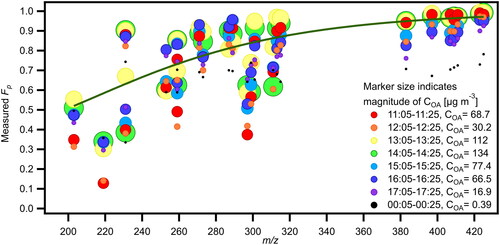
Figure 5. F_p versus m/z for a group of abundant compounds during 8 consecutive sampling periods under different OA loading conditions on TG2. Size of markers indicates magnitude of C_OA and their color indicates the sampling period. The solid (green) line is a fit based on 14:05-14:25 and is added to guide the eye.

An additional method of inferring volatility from FIGAERO-CIMS data is the use of maximum desorption temperature, T_max (Bannan et al. 2018; Lopez-Hilfiker et al. 2014). We compared T_max values to partitioning numbers, F_p, for HR-identified species (Figure S6) and for unit mass resolution (UMR) data (Figure S7) and found that even though there is a positive correlation between both measures of volatility, the correlation is fairly poor, especially for UMR data. The correlation is slightly stronger for high-resolution data, but with considerable scatter especially for species within the F_p range of 0.8 to 1.0 (presumably lower volatility species). One benefit of using both measures is that thermal decomposition products (compounds with high T_max and low F_p) are visually identifiable (see Figure S6).

Figure 6. (a): F_p versus log(C⁰) obtained from Li, Pöschl, and Shiraiwa (2016) correlation for two events: a high activity and a low activity period on Thanksgiving Day 2 (TG2). The black line indicates expected partitioning behavior at C_OA = 100 μg m³ whereas actual C_OA = 133.9 (b) Experimental log(C*) from FIGAERO-CIMS (calculated from F_p) versus log(C⁰) from Li, Pöschl, and Shiraiwa (2016) parameterization based on elemental formulas of HOMEChem compounds, for seven different cooking events.

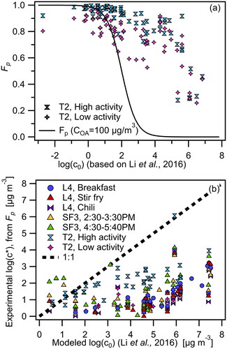
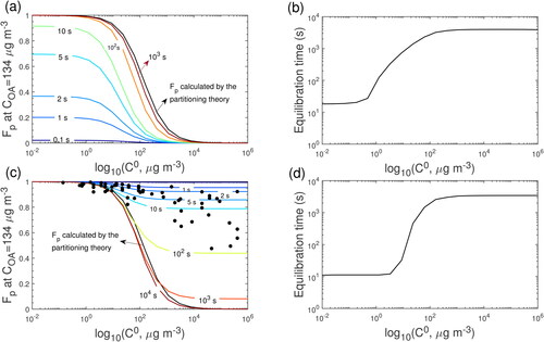
Figure 7. Predicted F_p variations with time for (a-b) condensation and (c-d) evaporation in the closed system and the F_p calculated by partitioning theory. C_OA is 134 μg m⁻³; T is 322.8 K and D_b is 3 × 10⁻¹² cm² s⁻¹.

An interesting feature of two-dimensional thermograms from HOMEChem is the trend in T_max versus m/z. There is a noticeable increase in T_max with increasing m/z, from m/z 250-800. This differs from 2 D-thermograms from environmental chamber data (Masoud and Hildebrandt Ruiz 2021; Wang and Hildebrandt Ruiz 2018) where T_max appears independent of m/z (up to m/z 350) and where thermal decomposition products (characterized by low m/z and high T_max) are clearly visible (see Figure S8). This is likely due to the difference in formation mechanisms for the observed products: for environmental chamber experiments, products are formed from photochemical reactions that occur at room temperature (25 °C), whereas for cooking experiments at HOMEChem, particle-phase products were likely emitted directly from cooking at high temperatures which makes them inherently more thermally stable. The chamber experiments were also highly controlled (a single VOC precursor was used) whereas during HOMEChem, a large variety of VOCs were present, which have different volatility behaviors.

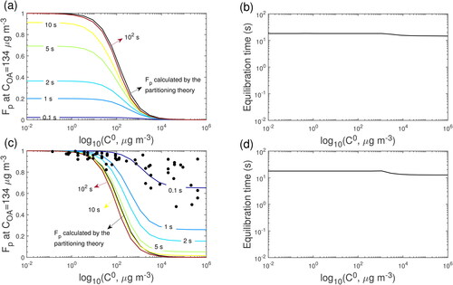
Figure 8. Predicted F_p variations with time for (a-b) condensation and (c-d) evaporation in the closed system and the F_p calculated by the partitioning theory. C_OA is 134 μg m⁻³; T is 298 K and D_b is 1 × 10⁻¹⁴ cm² s⁻¹.

3.2.1. Effect of dilution on partitioning

To study dilution effects on partitioning of compounds between gas and particle phases, we focused on one Thanksgiving Day (TG2) where cooking and cleaning activities were spaced out throughout the day and organic aerosol concentrations changed according to activity levels. We focused the analysis on select non-nitrogenated compounds that had the highest overall concentrations (in the gas and particle phases) during 8 consecutive sampling periods on TG2 (11:00AM to midnight the next day). The marker size in Figure 5 indicates organic aerosol concentration during the sampling period (C_OA range from 0.4-134 µg m⁻³) (Katz, Guo, et al. 2021), and the marker color indicates the time of day during which the particles were collected. As seen in Figure 5, as the concentration of organic aerosol increased, the partitioning number for compounds of the same saturation concentration generally increased as well, consistent with absorptive partitioning. The trend is particularly evident in the higher m/z range where F_p≥0.7. A closer examination of three time periods (14:05-14:25, 17:05-17:25, 00:05-00:25 (next day)) when C_OA values were about an order of magnitude apart (see Figure S9) shows that decreasing C_OA leads to correspondingly decreasing F_p values. The observable effect of dilution on partitioning suggests that FIGAERO-CIMS-measured F_p is a reliable indicator of partitioning behavior. This behavior also points to the importance of dilution in decreasing particle phase concentrations: increasing ventilation in the indoor environment can reduce particulate matter levels by adding cleaner air and by driving partitioning of compounds back into the gas phase due to lower concentrations. A similar analysis to Figure 5 with marker size corresponding to total particle signal from the FIGAERO is presented in Figure S10a, and reasonable correlation is seen between the FIGAERO total particle signal [ions/s] and AMS C_OA values [μg m⁻³] (Figure S10b).

3.2.2. Comparing partitioning values to saturation concentration

Given the inability of FIGAERO-CIMS data to provide structural information, we use an empirical parameterization by Li, Pöschl, and Shiraiwa (2016) to calculate saturation concentration C⁰ values based on elemental compositions, using the subset of measured species which contain C, H, and O atoms only and exhibit unimodal desorption behavior (see Sec. 3.2.1). The parameterization was developed by plotting the molar masses of a large number of compounds against their saturation concentration values predicted by EPI Suite. A “molecular corridor” is established accordingly, and parameters are fit so that we can estimate the saturation of a compound given its molar mass (see Section S9 and Figure S11). We use this method to calculate C⁰ values for a list of compounds that were emitted at high concentrations during 2 time periods on Thanksgiving day 2 – a high activity period (cooking, occupancy, cleaning) from 14:05-14:25, and a low activity period (unoccupied house) from 17:05-17:25. For the two time periods shown in Figure 6a, we added the gas and particle concentrations of each compound and determined the highest overall concentrations for each time period. We focused the analysis on ∼40 compounds which had the highest concentrations from each event and which together constituted 65% of the total signal during this time. We calculated partitioning numbers F_p for these compounds and plotted those against their corresponding empirically calculated saturation concentration, log(C⁰). As the saturation concentration of a compound, log(C⁰), increases, its partitioning number, F_p, decreases. The trend follows expected partitioning behavior where compounds with lower saturation concentration (i.e., lower volatility) preferentially partition into the particle phase. However, the points do not fall on the expected F_p at C_OA=100 μg m⁻³ line (black line) indicating that equilibrium conditions are not met. Note that the actual C_OA during the high activity and low activity periods were 134 and 16.9 μg m⁻³ respectively.

We calculated the experimental effective saturation concentration, C*, from measured F_p values based on Equation (4)(4) $$C_i^{*}=\frac{(1-F_p)}{F_p}\times C_{OA}$$(4) for the identified compounds and compared these values to the predicted saturation concentration, C⁰, from the Li, Pöschl, and Shiraiwa (2016) correlation, as seen in Figure 6b. The analysis includes seven time periods from three different days during the campaign. Several compounds that were observed during TG2 (high activity period) with C⁰ ≤10² µg m⁻³ fall on the 1:1 line. However, for most of the events, the points fall below the 1:1 line, which indicates that their experimental effective saturation concentration (based on measured partitioning, F_p) is lower than the predicted saturation concentration (based on the elemental formula parameterization (Li, Pöschl, and Shiraiwa 2016)). This indicates that the measured mass fraction of OA is higher than what would be expected based on predicted equilibrium partitioning. One explanation for this behavior is that the equilibration timescales for the events were longer than sampling timescales. The sampling inlet was placed at close proximity to the source which means that some compounds may have been sampled before fully partitioning. Another explanation for the difference between C⁰ (pure compound saturation concentration) and C* (effective saturation concentration, where C*=γC⁰) is the assumption of ideal thermodynamic mixing conditions, where the activity coefficient γ is assumed to be unity. This assumption does not take into account mixing effects of different organics (their activity coefficients), interactions with water, and interactions with other inorganic constituents of the sampled aerosol (Donahue et al. 2014; Shiraiwa et al. 2013; Zuend and Seinfeld 2012). A brief comparison of experimentally measured F_p values and literature-based saturation concentrations (assuming a specific structural formula) is presented in Sec. S10 (Figure S12). While F_p and saturation concentration values show a negative correlation, they do not follow the expected trend based on absorptive partitioning theory (Donahue et al. 2006) likely due to the assumptions of structural identity, and general difficulty in obtaining experimental vapor pressures for low volatility compounds.

3.2.3. Equilibration timescales and particle phase states

To investigate equilibration timescales, we used KM-GAP to simulate gas-particle partitioning of measured compounds dominated by condensation or evaporation. The condensation scenarios are simulated with initial conditions of C_p,0 (concentration in the particle phase) = 0 μg m⁻³ and C_g,0 (concentration in the gas phase) = 22 μg m⁻³. Figure 7a shows the temporal evolution of the predicted F_p for condensing compounds with C⁰ varied from 10⁻² to 10⁶ μg m⁻³ at measured C_OA of 134 μg m⁻³ and T of 322.8 K (conditions at Thanksgiving 2 from 14:05-14:25). The calculated viscosity is 2.2 × 10³ Pa s, indicating that the cooking OA adopts a semi-solid state. We note that the directly measured viscosity of organic mixtures collected from the surface near the stove during HOMEChem was <10⁴ Pa s (O’Brien et al. 2021). The sampled film contained organic material with similar composition to cooking OA measured via an online AMS during HOMEChem, indicating that cooking OA may adopt a low viscosity semi-solid phase state similar to the observed viscosity of organic films (O’Brien et al. 2021). We show equilibrium F_p values calculated by partitioning theory (Pankow 1994) at C_OA of 134 μg m⁻³, assuming ideal mixing conditions. When the system reaches full equilibrium, the predicted F_p should be very close to the F_p calculated by partitioning theory. Figure 7b shows the simulated τ_eq as a function of C⁰ showing that τ_eq is ∼18 s. Figure 7c shows the evaporation scenarios with initial conditions of C_p,0 = 20 μg m⁻³ and C_g,0 = 0 μg m⁻³. The experimentally detected compounds with measured F_p and C⁰ estimated by Li, Pöschl, and Shiraiwa (2016) are shown in black dots. Interestingly, the measured F_p of IVOC is close to the simulated F_p at t = 0.1 s. The simulated τ_eq is very close to the τ_eq in the condensation scenarios (Figure 7d).

We ran sensitivity simulations at room temperature (T = 25 °C) with D_b of 1 × 10⁻¹⁴ cm² s⁻¹ as seen in Figure 8. At C_OA of 134 μg m⁻³, comparing with the scenarios at T of 322.8 K (Figure 7), τ_eq of compounds with C⁰ > 1 μg m⁻³ significantly increases and can be longer than 10³ s (Figure 8b), indicating that gas-particle partitioning of these compounds is limited by bulk diffusion. For compounds with C⁰ < 1 μg m⁻³, τ_eq does not increase when T decreases, as the gas-particle partitioning of these lower volatility compounds is in the interfacial-transport limited regime (Mai et al. 2015). For the evaporation scenarios, the measured F_p of IVOC are mainly between the simulated F_p at t = 1 s and 10 s (Figure 8c).

The simulations indicate that timescales for partitioning compounds to reach equilibrium may be up to ∼14 s at 322.8 K and up to 15 min at 298 K. Thus, the particles could be out of equilibrium since the cooking activities were highly dynamic in nature (i.e., compounds were emitted in an intermittent manner) and the residence time in the lines (2.7 seconds) was shorter than this equilibration timescale. This may partly explain the discrepancy between the measured and estimated saturation concentrations (Figure 6b) which assumed equilibrium partitioning. Gas-particle partitioning of higher volatility compounds is limited mainly by the bulk diffusion in the semi-solid matrix.

4. Conclusion

We identified ∼480 unique molecular formulas measured by the FIGAERO-CIMS during several cooking events at the HOMEChem campaign and presented for the first time FIGAERO-CIMS-measured partitioning values for cooking aerosol generated in a realistic home environment. Molecular formulas containing C, H, O, N, Cl, and S atoms were identified and attributed to potential sources. Compounds containing C, H, O atoms only (CHO group) constituted the majority of emissions in the particle phase (∼74-85%), followed by the CHNO group (∼12-19%). Gas-particle partitioning of species showed a dependence on molecular weight, functional groups, and dilution, which was correlated with a decrease in PM concentration and fraction of measured compounds in the particle phase. Partitioning values, F_p, provided useful insight into volatility, and their use in tandem with T_max helped with the identification of thermal decomposition products. F_p values were generally well correlated with saturation concentration values obtained from the Li, Pöschl, and Shiraiwa (2016) parameterization based on elemental formulas. However, our comparison of experimentally determined saturation vapor concentrations (calculated from FIGAERO-CIMS-measured F_p) to saturation vapor concentration values obtained from the parameterization showed a discrepancy between the two methods, likely related to the assumption of equilibrium conditions at the time of sampling. We ran the KM-GAP model to investigate equilibration timescales at different organic aerosol concentrations and sampling temperatures, and found that it can take up to 14 seconds to reach equilibrium at the experimental conditions (T = 322 K) (up to 15 min at T = 298 K), whereas sampling timescales were shorter (2.7 seconds). Comparison of experimentally and empirically derived saturation concentrations suggests that compounds may have been released primarily in the particle phase during cooking events and were sampled before they fully equilibrated with the gas phase. The results presented in this work highlight the utility of data from the FIGAERO-CIMS in that it provided data on molecular composition, partitioning, and valuable inputs for kinetic and viscosity modeling. Overall, our analysis highlights the rich variety of compounds a person may be exposed to while cooking in their home. The impact of dilution on reducing cooking aerosol concentrations indicates the importance of increasing ventilation indoors (e.g., by opening windows) to reduce human exposure to particle-phase pollutants. The high concentrations of organic aerosol and the large variety of compounds present during cooking events emphasizes the importance of considering human exposure to pollutants in indoor air, especially in homes, and motivates further investigation into indoor air pollution mitigation measures.

Disclosure statement

The authors report there are no competing interests to declare.

Additional information

Funding

This work was supported in part by the Alfred P. Sloan Foundation (G2018-11366; G-2017-9944; G-2019-12306; G-2020-13912), by the National Science Foundation under grant No. 165362 and by the Welch Foundation (F-1925-20170325; F-1925-20200401). We thank all sponsors for their support. We also thank Dr. Atila Novoselac, Dr. Steve Bourne, Logan Hageman, and the entire HOMEChem Science team for their support during the project.

References

- Abdullahi, K. L., J. M. Delgado-Saborit, and R. M. Harrison. 2013. Emissions and indoor concentrations of particulate matter and its specific chemical components from cooking: A review. Atmos. Environ. 71:260–94. doi:10.1016/j.atmosenv.2013.01.061.
- Allan, J. D., P. I. Williams, W. T. Morgan, C. L. Martin, M. J. Flynn, J. Lee, E. Nemitz, G. J. Phillips, M. W. Gallagher, and H. Coe. 2009. Contributions from transport, solid fuel burning and cooking to primary organic aerosols in two UK cities. Atmos. Chem. Phys. 9 (5):19103–57.
- Anderson, J. O., J. G. Thundiyil, and A. Stolbach. 2012. Clearing the air: A review of the effects of particulate matter air pollution on human health. J. Med. Toxicol. 8 (2):166–75. doi:10.1007/s13181-011-0203-1.
- Bannan, T. J., M. Le Breton, M. Priestley, S. D. Worrall, A. Bacak, N. A. Marsden, A. Mehra, J. Hammes, M. Hallquist, M. R. Alfarra, et al. 2018. A method for extracting calibrated volatility information from the FIGAERO-HR-ToF-CIMS and its experimental application. Atmos. Meas. Tech. 12 (3):1429–39.
- Bergauff, M. A. 2010. Quantification and reduction of exposure to residential woodsmoke particulate matter. Graduate Student Theses, Dissertations, & Professional Papers, 789, The University of Montana. https://scholarworks.umt.edu/etd/789
- Boedicker, E. K., E. W. Emerson, G. R. McMeeking, S. Patel, M. E. Vance, and D. K. Farmer. 2021. Fates and spatial variations of accumulation mode particles in a multi-zone indoor environment during the HOMEChem campaign. Environ. Sci: Processes Impacts 23 (7):1029–39. doi:10.1039/D1EM00087J.
- Brown, W. L., D. A. Day, H. Stark, D. Pagonis, J. E. Krechmer, X. Liu, D. J. Price, E. F. Katz, P. F. DeCarlo, C. G. Masoud, et al. 2021. Real-time organic aerosol chemical speciation in the indoor environment using extractive electrospray ionization mass spectrometry. Indoor Air. 31 (1):141–55. doi:10.1111/ina.12721.
- Buchholz, A., A. Ylisirniö, W. Huang, C. Mohr, M. Canagaratna, D. R. Worsnop, S. Schobesberger, and A. Virtanen. 2019. Deconvolution of FIGAERO-CIMS thermal desorption profiles using positive matrix factorisation to identify chemical and physical processes during particle evaporation. Atmos. Chem. Phys. 2019 (November):1–36.
- Burnett, R., H. Chen, M. Szyszkowicz, N. Fann, B. Hubbell, C. A. Pope, J. S. Apte, M. Brauer, A. Cohen, S. Weichenthal, et al. 2018. Global estimates of mortality associated with long-term exposure to outdoor fine particulate matter. Proc. Natl. Acad. Sci. U S A 115 (38):9592–7. doi:10.1073/pnas.1803222115.
- Cain, K. P., E. Karnezi, and S. N. Pandis. 2020. Challenges in determining atmospheric organic aerosol volatility distributions using thermal evaporation techniques. Aerosol Sci. Technol. 54 (8):941–57. doi:10.1080/02786826.2020.1748172.
- Charan, S. M., Y. Huang, R. S. Buenconsejo, Q. Li, D. R. Cocker, and J. H. Seinfeld. 2022. Secondary organic aerosol formation from the oxidation of decamethylcyclopentasiloxane at atmospherically relevant OH concentrations. Atmos. Chem. Phys. 22 (2):917–28. doi:10.5194/acp-22-917-2022.
- Chenyakin, Y., A. D. Ullmann, E. Evoy, L. Renbaum-Wolff, S. Kamal, and K. A. Bertram. 2017. Diffusion coefficients of organic molecules in sucrose-water solutions and comparison with Stokes-Einstein predictions. Atmos. Chem. Phys. 17 (3):2423–35. doi:10.5194/acp-17-2423-2017.
- Coggon, M. M., B. C. McDonald, A. Vlasenko, P. R. Veres, F. Bernard, A. R. Koss, B. Yuan, J. B. Gilman, J. Peischl, K. C. Aikin, et al. 2018. Diurnal variability and emission pattern of decamethylcyclopentasiloxane (D5) from the application of personal care products in two north American cities. Environ. Sci. Technol. 52 (10):5610–8. doi:10.1021/acs.est.8b00506.
- Crippa, M., P. F. Decarlo, J. G. Slowik, C. Mohr, M. F. Heringa, R. Chirico, L. Poulain, F. Freutel, J. Sciare, J. Cozic, et al. 2013. Wintertime aerosol chemical composition and source apportionment of the organic fraction in the metropolitan area of Paris. Atmos. Chem. Phys. 13 (2):961–81. doi:10.5194/acp-13-961-2013.
- D’Ambro, E. L., B. H. Lee, J. Liu, J. E. Shilling, C. J. Gaston, F. D. Lopez-Hilfiker, S. Schobesberger, R. A. Zaveri, C. Mohr, A. Lutz, et al. 2017. Molecular composition and volatility of isoprene photochemical oxidation secondary organic aerosol under low- and high-NOx conditions. Atmos. Chem. Phys. 17 (1):159–74. doi:10.5194/acp-17-159-2017.
- DeCarlo, P. F., J. R. Kimmel, A. Trimborn, M. J. Northway, J. T. Jayne, A. C. Aiken, M. Gonin, K. Fuhrer, T. Horvath, K. S. Docherty, et al. 2006. Field-deployable, high-resolution, time-of-flight aerosol mass spectrometer. Anal. Chem. 78 (24):8281–9. doi:10.1021/ac061249n.
- DeRieux, W. S. W., Y. Li, P. Lin, J. Laskin, A. Laskin, A. K. Bertram, S. A. Nizkorodov, and M. Shiraiwa. 2018. Predicting the glass transition temperature and viscosity of secondary organic material using molecular composition. Atmos. Chem. Phys. 18 (9):6331–51. doi:10.5194/acp-18-6331-2018.
- Dette, H. P., M. Qi, D. C. Schröder, A. Godt, and T. Koop. 2014. Glass-forming properties of 3-methylbutane-1,2,3-tricarboxylic acid and its mixtures with water and pinonic acid. J. Phys. Chem. A 118 (34):7024–33.
- Donahue, N. M., S. A. Epstein, S. N. Pandis, and A. L. Robinson. 2011. A two-dimensional volatility basis set: 1. organic-aerosol mixing thermodynamics. Atmos. Chem. Phys. 11 (7):3303–18. doi:10.5194/acp-11-3303-2011.
- Donahue, N. M., A. L. Robinson, C. O. Stanier, and S. N. Pandis. 2006. Coupled partitioning, dilution, and chemical aging of semivolatile organics. Environ. Sci. Technol. 40 (8):2635–43.
- Donahue, N. M., A. L. Robinson, E. R. Trump, I. Riipinen, and J. H. Kroll. 2014. Volatility and aging of atmospheric organic aerosol. In Atmospheric and aerosol chemistry. Topics in current chemistry (V339), ed. V.F. McNeill, P.A. Ariya, 97–143. Berlin, Heidelberg: Springer.
- Drewnick, F., S. S. Hings, P. DeCarlo, J. T. Jayne, M. Gonin, K. Fuhrer, S. Weimer, J. L. Jimenez, K. L. Demerjian, S. Borrmann, et al. 2005. A new time-of-flight aerosol mass spectrometer (TOF-AMS) – Instrument description and first field deployment. Aerosol Sci. Technol. 39 (7):637–58. doi:10.1080/02786820500182040.
- Elser, M., R. J. Huang, R. Wolf, J. G. Slowik, Q. Wang, F. Canonaco, G. Li, C. Bozzetti, K. R. Daellenbach, Y. Huang, et al. 2016. New insights into PM2.5 chemical composition and sources in two major cities in China during extreme haze events using aerosol mass spectrometry. Atmos. Chem. Phys. 16 (5):3207–25. doi:10.5194/acp-16-3207-2016.
- Farmer, D. K., M. E. Vance, J. P. D. Abbatt, A. Abeleira, M. R. Alves, C. Arata, E. Boedicker, S. Bourne, F. Cardoso-Saldaña, R. Corsi, et al. 2019. Overview of HOMEChem: House observations of microbial and environmental chemistry. Environ. Sci. Process. Impacts. 21 (8):1280–300.
- Fu, Z., H. B. Xie, J. Elm, X. Guo, Z. Fu, Z. Fu, and J. Chen. 2020. Formation of low-volatile products and unexpected high formaldehyde yield from the atmospheric oxidation of methylsiloxanes. Environ. Sci. Technol. 54 (12):7136–45.
- Grieshop, A. P., M. A. Miracolo, N. M. Donahue, and A. L. Robinson. 2009. Constraining the volatility distribution and gas-particle partitioning of combustion aerosols using isothermal dilution and thermodenuder measurements. Environ. Sci. Technol. 43 (13):4750–6.
- Holeček, M. 2020. Histidine in health and disease: Metabolism, Physiological importance, and use as a supplement. Nutrients 12 (3):848. doi:10.3390/nu12030848.
- Huang, W., H. Saathoff, A. Pajunoja, X. Shen, K.-H. Naumann, R. Wagner, A. Virtanen, T. Leisner, and C. Mohr. 2018. α-Pinene secondary organic aerosol at low temperature: Chemical composition and implications for particle viscosity. Atmos. Chem. Phys. 18 (4):2883–98. doi:10.5194/acp-18-2883-2018.
- Huboyo, H. S., S. Tohno, and R. Cao. 2011. Indoor PM2.5 characteristics and CO concentration related to water-based and oil-based cooking emissions using a gas stove. Aerosol Air Qual. Res. 11 (4):401–11. doi:10.4209/aaqr.2011.02.0016.
- Huffman, J. A., K. S. Docherty, A. C. Aiken, M. J. Cubison, I. M. Ulbrich, P. F. Decarlo, D. Sueper, J. T. Jayne, D. R. Worsnop, P. J. Ziemann, et al. 2009. Chemically-resolved aerosol volatility measurements from two megacity field studies. Atmos. Chem. Phys. 9 (18):7161–82. doi:10.5194/acp-9-7161-2009.
- Huffman, J. A., P. J. Ziemann, J. T. Jayne, D. R. Worsnop, and J. L. Jimenez. 2008. Development and characterization of a fast-stepping/scanning thermodenuder for chemically-resolved aerosol volatility measurements. Aerosol Sci. Technol. 42 (5):395–407. doi:10.1080/02786820802104981.
- Ito, H. 1977. The formation of maltol and isomaltol through degradation of sucrose. Agric. Biol. Chem. 41 (7):1307–8.
- Jayne, J. T., D. C. Leard, X. Zhang, P. Davidovits, K. A. Smith, C. E. Kolb, and D. R. Worsnop. 2000. Development of an aerosol mass spectrometer for size and composition analysis of submicron particles. Aerosol Sci. Technol. 33 (1–2):49–70. doi:10.1080/027868200410840.
- Jiménez-Guerrero, P, and N. Ratola. 2021. Characterizing the regional concentrations and seasonality of the emerging pollutant decamethylcyclopentasiloxane (D5) using a WRFþCHIMERE modeling approach. Elementa, 9 (1):00137.
- Karnezi, E., I. Riipinen, and S. N. Pandis. 2014. Measuring the atmospheric organic aerosol volatility distribution: A theoretical analysis. Atmos. Meas. Tech. 7 (9):2953–65. doi:10.5194/amt-7-2953-2014.
- Katz, E. F., H. Guo, P. Campuzano-Jost, D. A. Day, W. L. Brown, E. Boedicker, M. Pothier, D. M. Lunderberg, S. Patel, K. Patel, et al. 2021. Quantification of cooking organic aerosol in the indoor environment using aerodyne aerosol mass spectrometers. Aerosol Sci. Technol. 55 (10):1099–114. doi:10.1080/02786826.2021.1931013.
- Katz, E. F., D. M. Lunderberg, W. L. Brown, D. A. Day, J. L. Jimenez, W. W. Nazaroff, A. H. Goldstein, and P. F. Decarlo. 2021. Large emissions of low-volatility siloxanes during residential oven use. Environ. Sci. Technol. Lett. 8 (7):519–24. doi:10.1021/acs.estlett.1c00433.
- Klein, F., N. J. Farren, C. Bozzetti, K. R. Daellenbach, D. Kilic, N. K. Kumar, S. M. Pieber, J. G. Slowik, R. N. Tuthill, J. F. Hamilton, et al. 2016. Indoor terpene emissions from cooking with herbs and pepper and their secondary organic aerosol production potential. Sci. Rep. 6:36623.
- Klepeis, N. E., W. C. Nelson, W. R. Ott, J. P. Robinson, A. M. Tsang, P. Switzer, J. V. Behar, S. C. Hern, and W. H. Engelmann. 2001. The national human activity pattern survey. Lawrence Berkeley Natl. Lab 11 (3):231–52.
- Koop, T., J. Bookhold, M. Shiraiwa, and U. Pöschl. 2011. Glass transition and phase state of organic compounds: Dependency on molecular properties and implications for secondary organic aerosols in the atmosphere. Phys. Chem. Chem. Phys. 13 (43):19238–55.
- Kroll, J. H., C. Y. Lim, S. H. Kessler, and K. R. Wilson. 2015. Heterogeneous oxidation of atmospheric organic aerosol: Kinetics of changes to the amount and oxidation state of particle-phase organic carbon. J. Phys. Chem. A 119 (44):10767–83. doi:10.1021/acs.jpca.5b06946.
- Lee, B. H., F. D. Lopez-Hilfiker, C. Mohr, T. Kurtén, D. R. Worsnop, and J. A. Thornton. 2014. An iodide-adduct high-resolution time-of-flight chemical-ionization mass spectrometer: Application to atmospheric inorganic and organic compounds. Environ. Sci. Technol. 48 (11):6309–17. doi:10.1021/es500362a.
- Li, Y., T. M. Fu, J. Z. Yu, X. Feng, L. Zhang, J. Chen, S. K. R. Boreddy, K. Kawamura, P. Fu, X. Yang, et al. 2021. Impacts of chemical degradation on the global budget of atmospheric levoglucosan and its use as a biomass burning tracer. Environ. Sci. Technol. 55 (8):5525–36.
- Li, Y., U. Pöschl, and M. Shiraiwa. 2016. Molecular corridors and parameterizations of volatility in the chemical evolution of organic aerosols. Atmos. Chem. Phys. 16 (5):3327–44. doi:10.5194/acp-16-3327-2016.
- Li, Y, and M. Shiraiwa. 2019. Timescales of secondary organic aerosols to reach equilibrium at various temperatures and relative humidities. Atmos. Chem. Phys. 19 (9):5959–71. doi:10.5194/acp-19-5959-2019.
- Li, Y., A. Tasoglou, A. Liangou, K. P. Cain, L. Jahn, P. Gu, E. Kostenidou, and S. N. Pandis. 2018. Cloud condensation nuclei activity and hygroscopicity of fresh and aged cooking organic aerosol. Atmos. Environ. 176:103–9. doi:10.1016/j.atmosenv.2017.11.035.
- Li, Y., Y. Wu, J. Xu, A. Wu, Z. Zhao, M. Tong, and S. Luan. 2021. Chemical characterization of particulate organic matter from commercial restaurants: Alkyl PAHs as new tracers for cooking. Sci. Total Environ. 770:145308. doi:10.1016/j.scitotenv.2021.145308.
- Liu, T., Z. Wang, X. Wang, and C. K. Chan. 2018. Primary and secondary organic aerosol from heated cooking oil emissions. Atmos. Chem. Phys. 18 (15):11363–74. doi:10.5194/acp-18-11363-2018.
- Lopez-Hilfiker, F. D., C. Mohr, M. Ehn, F. Rubach, E. Kleist, J. Wildt, T. F. Mentel, A. J. Carrasquillo, K. E. Daumit, J. F. Hunter, et al. 2015. Phase partitioning and volatility of secondary organic aerosol components formed from α-pinene ozonolysis and OH oxidation: The importance of accretion products and other low volatility compounds. Atmos. Chem. Phys. 15 (14):7765–76. doi:10.5194/acp-15-7765-2015.
- Lopez-Hilfiker, F. D., C. Mohr, M. Ehn, F. Rubach, E. Kleist, J. Wildt, T. F. Mentel, A. Lutz, M. Hallquist, D. Worsnop, et al. 2014. A novel method for online analysis of gas and particle composition: Description and evaluation of a filter inlet for gases and AEROsols (FIGAERO). Atmos. Meas. Tech. 7 (4):983–1001. doi:10.5194/amt-7-983-2014.
- Louvaris, E. E., E. Karnezi, E. Kostenidou, C. Kaltsonoudis, and S. N. Pandis. 2017. Estimation of the volatility distribution of organic aerosol combining thermodenuder and isothermal dilution measurements. Atmos. Meas. Tech. 10 (10):3909–18. doi:10.5194/amt-10-3909-2017.
- Lunderberg, D. M., K. Kristensen, Y. Tian, C. Arata, P. K. Misztal, Y. Liu, N. Kreisberg, E. F. Katz, P. F. Decarlo, S. Patel, et al. 2020. Surface emissions modulate indoor SVOC concentrations through volatility-dependent partitioning. Environ. Sci. Technol. 54 (11):6751–60.
- Luning, P. A., T. Ebbenhorst‐Seller, T. de Rijk, and J. P. Roozen. 1995. Effect of hot-air drying on flavour compounds of bell peppers (Capsicum annuum). J. Sci. Food Agric. 68 (3):355–65. doi:10.1002/jsfa.2740680315.
- Mai, H., M. Shiraiwa, R. C. Flagan, and J. H. Seinfeld. 2015. Under what conditions can equilibrium gas–particle partitioning be expected to hold in the atmosphere?. Environ. Sci. Technol. 49 (19):11485–91. doi:10.1021/acs.est.5b02587.
- Masoud, C. G, and L. Hildebrandt Ruiz. 2021. Chlorine-initiated oxidation of α-pinene: Formation of secondary organic aerosol and highly oxygenated organic molecules. ACS Earth Space Chem. 5 (9):2307–19. doi:10.1021/acsearthspacechem.1c00150.
- Mattila, J. M., P. S. J. Lakey, M. Shiraiwa, C. Wang, J. P. D. Abbatt, C. Arata, A. H. Goldstein, L. Ampollini, E. F. Katz, P. F. Decarlo, et al. 2020. Multiphase chemistry controls inorganic chlorinated and nitrogenated compounds in indoor air during bleach cleaning. Environ. Sci. Technol. 54 (3):1730–9. doi:10.1021/acs.est.9b05767.
- Mcdonald, J. D., B. Zielinska, E. M. Fujita, J. C. Sagebiel, J. C. Chow, and J. G. Watson. 2003. Emissions from charbroiling and grilling of chicken and beef. J. Air Waste Manage. Assoc. 53 (2):185–94. doi:10.1080/10473289.2003.10466141.
- Mikhailov, E., S. Vlasenko, S. T. Martin, T. Koop, and U. Pöschl. 2009. Amorphous and crystalline aerosol particles interacting with water vapor: Conceptual framework and experimental evidence for restructuring, phase transitions and kinetic limitations. Atmos. Chem. Phys. 9 (24):9491–522. doi:10.5194/acp-9-9491-2009.
- Mohr, C., P. F. DeCarlo, M. F. Heringa, R. Chirico, J. G. Slowik, R. Richter, C. Reche, A. Alastuey, X. Querol, R. Seco, et al. 2012. Identification and quantification of organic aerosol from cooking and other sources in Barcelona using aerosol mass spectrometer data. Atmos. Chem. Phys. 12 (4):1649–65. doi:10.5194/acp-12-1649-2012.
- Mohr, C., J. A. Huffman, M. J. Cubison, A. C. Aiken, K. S. Docherty, J. R. Kimmel, I. M. Ulbrich, M. Hannigan, and J. L. Jimenez. 2009. Characterization of primary organic aerosol emissions from meat cooking, trash burning, and motor vehicles with high-resolution aerosol mass spectrometry and comparison with ambient and chamber observations. Environ. Sci. Technol. 43 (7):2443–9. doi:10.1021/es8011518.
- Murphy, B. N., N. M. Donahue, C. Fountoukis, and S. N. Pandis. 2011. Simulating the oxygen content of ambient organic aerosol with the 2D volatility basis set. Atmos. Chem. Phys. 11 (15):7859–73. doi:10.5194/acp-11-7859-2011.
- Nasir, Z. A, and I. Colbeck. 2013. Particulate pollution in different housing types in a UK suburban location. Sci. Total Environ. 445–446:165–76. doi:10.1016/j.scitotenv.2012.12.042.
- Nel, A. 2005. Air pollution–related illness: Effects of particles. Science 308 (5723):804–6. doi:10.1126/science.1108752.
- Nováková, Z., J. Novák, Z. Kitanovski, P. Kukučka, M. Smutná, M. Wietzoreck, G. Lammel, and K. Hilscherová. 2020. Toxic potentials of particulate and gaseous air pollutant mixtures and the role of PAHs and their derivatives. Environ. Int. 139:105634
- O’Brien, R. E., Y. Li, K. J. Kiland, E. F. Katz, V. W. Or, E. Legaard, E. Q. Walhout, C. Thrasher, V. H. Grassian, P. F. DeCarlo, et al. 2021. Emerging investigator series: Chemical and physical properties of organic mixtures on indoor surfaces during HOMEChem. Environ. Sci: Processes Impacts 23 (4):559–68. doi:10.1039/D1EM00060H.
- Pankow, J. F. 2001. A consideration of the role of gas/particle partitioning in the deposition of nicotine and other tobacco smoke compounds in the respiratory tract. Chem. Res. Toxicol. 14 (11):1465–81. doi:10.1021/tx0100901.
- Pankow, J. F. 1994. An absorption model of the gas/aerosol partitioning involved in the formation of secondary organic aerosol. Atmos. Environ. 28 (2):189–93. doi:10.1016/1352-2310(94)90094-9.
- Patel, S., S. Sankhyan, E. K. Boedicker, P. F. Decarlo, D. K. Farmer, A. H. Goldstein, E. F. Katz, W. W. Nazaroff, Y. Tian, J. Vanhanen, et al. 2020. Indoor particulate matter during HOMEChem: Concentrations, size distributions, and exposures. Environ. Sci. Technol. 54 (12):7107–16.
- Petters, M. D, and S. M. Kreidenweis. 2007. A single parameter representation of hygroscopic growth and cloud condensation nucleus activity. Atmos. Chem. Phys. 7 (8):1961–71. doi:10.5194/acp-7-1961-2007.
- Pope, C. A, and D. W. Dockery. 2006. Health effects of fine particulate air pollution: Lines that connect. J. Air Waste Manag. Assoc. 56 (6):709–42. doi:10.1080/10473289.2006.10464485.
- Reyes-Villegas, E., T. Bannan, M. Le Breton, A. Mehra, M. Priestley, C. Percival, H. Coe, and J. D. Allan. 2018. Online chemical characterization of food-cooking organic aerosols: Implications for source apportionment. Environ. Sci. Technol. 52 (9):5308–18. doi:10.1021/acs.est.7b06278.
- Riipinen, I., J. R. Pierce, N. M. Donahue, and S. N. Pandis. 2010. Equilibration time scales of organic aerosol inside thermodenuders: Evaporation kinetics versus thermodynamics. Atmos. Environ. 44 (5):597–607. doi:10.1016/j.atmosenv.2009.11.022.
- Schobesberger, S., E. L. Ambro, F. D. Lopez-Hilfiker, C. Mohr, and J. A. Thornton. 2018. A model framework to retrieve thermodynamic and kinetic properties of organic aerosol from composition-resolved thermal desorption measurements. Atmos. Chem. Phys. 18 (20):14757–85. doi:10.5194/acp-18-14757-2018.
- Shiraiwa, M., C. Pfrang, T. Koop, and U. Pöschl. 2012. Kinetic multi-layer model of gas-particle interactions in aerosols and clouds (KM-GAP): Linking condensation, evaporation and chemical reactions of organics, oxidants and water. Atmos. Chem. Phys. 12 (5):2777–94. doi:10.5194/acp-12-2777-2012.
- Shiraiwa, M., A. Zuend, A. K. Bertram, and J. H. Seinfeld. 2013. Gas-particle partitioning of atmospheric aerosols: Interplay of physical state, non-ideal mixing and morphology. Phys. Chem. Chem. Phys. 15 (27):11441–53.
- Sjaastad, A. K., R. B. Jørgensen, and K. Svendsen. 2010. Exposure to polycyclic aromatic hydrocarbons (PAHs), mutagenic aldehydes and particulate matter during pan frying of beefsteak. Occup. Environ. Med. 67 (4):228–32. doi:10.1136/oem.2009.046144.
- Slowik, J. G., Vlasenko, A. McGuire, M., Evans, G. J. Abbatt, and J. P. D. 2010. Simultaneous factor analysis of organic particle and gas mass spectra: AMS and PTR-MS measurements at an urban site. Atmos. Chem. Phys. 10 (4):1969–88. doi:10.5194/acp-10-1969-2010.
- Shi, X., T. Xia, B. E. McKamey, X. Wu, Y. Sun, W. Zhou, and G. Zhang. 2021. Concise and efficient synthesis of [6]-paradol. Org. Process Res. Dev. 25 (6):1360–5. doi:10.1021/acs.oprd.0c00553.
- Stark, H., R. L. N. Yatavelli, S. L. Thompson, H. Kang, J. E. Krechmer, J. R. Kimmel, B. B. Palm, W. Hu, P. L. Hayes, D. A. Day, et al. 2017. Impact of thermal decomposition on thermal desorption instruments: advantage of thermogram analysis for quantifying volatility distributions of organic species. Environ. Sci. Technol. 51 (15):8491–500. doi:10.1021/acs.est.7b00160.
- Voliotis, A., Y. Wang, Y. Shao, M. Du, T. Bannan, C. Percival, S. Pandis, M. R. Alfarra, and G. McFiggans. 2021. Exploring the composition and volatility of secondary organic aerosols in mixed anthropogenic and biogenic precursor systems. Atmos. Chem. Phys. 21 (18):14251–73. doi:10.5194/acp-21-14251-2021.
- Wallace, L. 2006. Indoor sources of ultrafine and accumulation mode particles: Size distributions, size-resolved concentrations, and source strengths. Aerosol Sci. Technol. 40 (5):348–60. doi:10.1080/02786820600612250.
- Wan, M. P., C. L. Wu, G. N. Sze To, T. C. Chan, and C. Y. H. Chao. 2011. Ultrafine particles, and PM2.5 generated from cooking in homes. Atmos. Environ. 45 (34):6141–8. doi:10.1016/j.atmosenv.2011.08.036.
- Wang, C., D. B. Collins, C. Arata, A. H. Goldstein, J. M. Mattila, D. K. Farmer, L. Ampollini, P. F. DeCarlo, A. Novoselac, M. E. Vance, et al. 2020. Surface reservoirs dominate dynamic gas-surface partitioning of many indoor air constituents. Sci. Adv. 6 (8):8973. doi:10.1126/sciadv.aay8973.
- Wang, D. S, and L. Hildebrandt Ruiz. 2018. Chlorine-initiated oxidation of alkanes under high-NO conditions: Insights into secondary organic aerosol composition and volatility using a FIGAERO-CIMS. Atmos. Chem. Phys. 18 (21):15535–53. doi:10.5194/acp-18-15535-2018.
- Wang, D. S, and L. Hildebrandt Ruiz. 2017. Secondary organic aerosol from chlorine-initiated oxidation of isoprene. Atmos. Chem. Phys. 17 (22):13491–508. doi:10.5194/acp-17-13491-2017.
- Yucuis, R. A., C. O. Stanier, and K. C. Hornbuckle. 2013. Cyclic siloxanes in air, including identification of high levels in Chicago and distinct diurnal variation. Chemosphere 92 (8):905–10. doi:10.1016/j.chemosphere.2013.02.051.
- Zobrist, B., C. Marcolli, D. A. Pedernera, and T. Koop. 2008. Do atmospheric aerosols form glasses? Atmos. Chem. Phys. 8 (17):5221–44. doi:10.5194/acp-8-5221-2008.
- Zuend, A, and J. H. Seinfeld. 2012. Modeling the gas-particle partitioning of secondary organic aerosol: The importance of liquid-liquid phase separation. Atmos. Chem. Phys. 12 (9):3857–82. doi:10.5194/acp-12-3857-2012.