Constraining the complex refractive index of black carbon particles using the complex forward-scattering amplitude

Abstract

Black carbon is the largest contributor to global aerosol’s shortwave absorption in the current atmosphere and is an important positive climate forcer. The complex refractive index, m = m_r + im_i, the primary determinant of the absorbed and scattered energies of incident radiation per unit volume of particulate material, has not been accurately known for atmospheric black carbon material. An accurate value at visible wavelengths has been difficult to obtain due to the black carbon’s wavelength-scale irregularity and variability of aggregate shape, distribution in particle size, and mixing with other aerosol compounds. Here, we present a method to constrain a plausible (m_r, m_i) domain for black carbon from the observed distribution of the complex forward-scattering amplitude S(0°). This approach suppresses the biases due to the above-mentioned complexities. The S(0°) distribution of black carbon is acquired by performing single particle S(0°) measurements in a water medium after collecting atmospheric aerosols into water. We demonstrate the method operating at λ = 0.633 μm for constraining the refractive index of black carbon aerosols in the north-western Pacific boundary layer. From the plausible (m_r, m_i) domain consistent with the observed S(0°) distributions and the reported range of mass absorption cross-section, we conservatively select 1.95 + 0.96i as a recommendable value of the refractive index for uncoated black carbon at visible wavelengths. The recommendable value is 0.17 larger in m_i than the widely used value 1.95 + 0.79i in current aerosol-climate models, implying a ∼16% underestimate of shortwave absorption by black carbon aerosols in current climate simulations.

Editor:

• Hans Moosmüller

1. Introduction

Black carbon (BC) emitted as an aerosol byproduct of the combustion of fossil fuels and biomasses, is one of the major anthropogenic contributors to positive climate forcing (Bond et al. 2013). In the present atmosphere, BC is estimated to generate the largest contribution to global aerosol shortwave absorption (Samset et al. 2018; Sand et al. 2021). In climate simulations, the remaining large uncertainty in aerosol shortwave absorption dominates the predictive uncertainty for precipitation (Samset 2022). BC is estimated to be the second largest contributor to positive effective radiative forcing among all greenhouse gases and aerosols over the Arctic, partly due to the effects of BC deposition on snow on surface albedo reduction (Oshima et al. 2020).

Freshly emitted BC particles can rapidly undergo internal mixing with other major aerosol components (e.g., sulfate, organics, water) through coagulation, condensation, and cloud processing to form “BC-containing particles” (Wang et al. 2017; Adachi et al. 2014, 2021). Here, we use the term BC to refer to the strongly light-absorbing insoluble carbonaceous material (Bond et al. 2013), which will be more rigorously defined as “ns-soot” according to electron microscopic analyses (Buseck et al. 2014) or as “soot-BC” according to the classification of ambient light-absorbing carbonaceous particles by Corbin et al. (2019). In this paper, we use the terms “BC particles”, and “BC aggregates” interchangeably to refer to an isolated particle consisting of detectable BC material only, and distinguished from BC-containing particles that may contain additional materials. Single atmospheric BC particles were observed to be fractal-like aggregates of nanospheres (Bond et al. 2013). The nanosphere diameters are within the 10–100 nm range (Buseck et al. 2014).

For such nonspherical BC aggregates, numerical light-scattering solvers, such as the superposition T-matrix method (STM) or discrete dipole approximation (DDA), are needed to theoretically predict optical properties. The mass absorption cross-section (MAC) of BC aggregates is predicted to be only weakly sensitive to the morphological parameters of aggregate (e.g., fractal dimension, monomer size), but strongly sensitive to the refractive index of the BC material (Liu and Mishchenko 2005). In climate modeling, basic assumptions about the BC refractive index therefore play a key role in aerosol shortwave absorption (Stier et al. 2007).

The refractive index m_r + im_i of atmospheric BC at visible wavelengths is often assumed to be one of the following: i) the highest recommended value for “light-absorbing carbon” at λ = 0.55 μm by Bond and Bergstrom (2006), 1.95 + 0.79i (BB06-h); ii) the lowest recommended value for light-absorbing carbon at λ = 0.55 μm by Bond and Bergstrom (2006), 1.75 + 0.63i (BB06-l); and iii) the wavelength-dependent m_r + im_i value experimentally determined for propane-air flame soot by Chang and Charalampopoulos (1990) (CC90), which is, for example, 1.74 + 0.59i at λ = 0.55 μm. In practical uses of the BB06-h and BB06-l, the BC refractive index is assumed to be wavelength independent. Table 1 shows a non-exhaustive list of recent publications on atmospheric sciences that used any of the BB06-l, BB06-h, and CC90.

Table 1. List of the publications using the BB06-h, BB06-l, and CC90 for BC refractive index.

Category	Authors and year	Research focus	BC refractive index values used/refereed
Light-scattering simulation	Moosmüller, Chakrabarty, and Arnott (2009)	Review of aerosol light absorption and its measurement techniques	BB06-h
	Kahnert and Devasthale (2011)	Spectral optical properties of pure BC aggregates	CC90
	Cheng et al. (2013)	Spectral optical properties of BC-containing particles	CC90
	Scarnato et al. (2013)	Mass absorption cross-section of NaCl-BC mixture	BB06-h
	Scarnato et al. (2015)	Spectral optical properties of a dust-BC mixture	CC90
	Wu et al. (2015)	Effect of monomer polydispersity of BC aggregates on its mass absorption cross-section	BB06-h
	Wu et al. (2018)	Morphological effects of absorption enhancement	CC90
	Beeler and Chakrabarty (2022)	Parameterization of mass absorption cross-section of BC-containing particles	BB06-h
Aerosol remote sensing	Koike et al. (2014)	Interpretation of aerosol absorption optical depth from in-situ aircraft data	BB06-h, Average of BB06-h and -l
	Schuster et al. (2016)	Distinguishing different absorbing aerosol species	BB06-h, BB06-l
	Li et al. (2019)	Retrieval of aerosol components	BB06-h, BB06-l
Aerosol-climate model	Stier et al. (2007)	Global distribution of aerosol absorption, climate model	BB06-h, BB06-l
	Zaveri et al. (2010)	Modeling aerosol’s microphysical properties, particle-resolved aerosol box model	Midpoint of BB06-h and -l
	Yu et al. (2012)	Aerosol microphysics module for climate models	Average of BB06-h and -l
	Brown et al. (2021)	Intercomparison of biomass aerosol absorption among climate models	BB06-h, BB06-l, Average of BB06-h and -l

The wavelength-dependent BC refractive index from the Optical Properties of Aerosols and Clouds (OPAC) database (Hess, Koepke, and Schult 1998), which is 1.75 + 0.44i at λ = 0.55 μm, is still used in some climate models (Sand et al. 2021), even though it was formally not recommended by Bond and Bergstrom (2006) because of the ambiguity of experimental evidence. We therefore do not include the OPAC value in our discussion.

The recommended values at λ = 0.55 μm by Bond and Bergstrom (2006), BB06-h and -l, were determined based on the hypothetical “upper void-fraction line” on the (m_r, m_i) plane, which is a linear extrapolation of available experimental values for non-graphitic light-absorbing carbon, including CC90, toward a point of intersection with the hypothetical “graphitization line”. The intersection point was defined as BB06-h, which is not close to any experimental data. The BB06-l is close to the CC09 at λ = 0.55 μm as it was used as the uppermost datapoint to draw the void-fraction line.

Chang and Charalampopoulos (1990) experimentally determined the wavelength-dependent refractive index of a propane-air flame soot, CC90, by applying the Kramers-Kronig dispersion theory to the measured spectral extinction coefficient of suspended soot particles over λ = 0.2–6.4 μm, for an observationally constrained particle-size distribution. The particle-size distribution was estimated using a photon-correlation technique at 0.488 μm wavelength (dynamic light-scattering). Chang and Charalampopoulos (1990) used the spherical particle-shape assumption in their interpretations of the spectral extinction and dynamic light-scattering data, possibly due to the unavailability of theoretical methods that accounted for more realistic shapes at that time. The spherical particle assumption, when applied to soot particles that are aggregates of nanospheres, can lead to a biased inference of spectral refractive index. For this reason, Chang and Charalampopoulos (1990) mentioned that their derived refractive index should be regarded as an “effective” refractive index subject to their specific assumptions.

There are more experimental studies on BC refractive index (cf. Table 4 and Figure 7 of Bond and Bergstrom 2006). Some of them are based on the extinction spectroscopy of suspended particles as Chang and Charalampopoulos (1990), but with either less detailed experimental design or less detailed theoretical analyses. Others are based on the reflectance spectroscopy of a compressed pellet of powder sample or reflectance and transmission spectroscopy of particles collected on a plate. In the compressed-pellet approach, the wavelength-scale inhomogeneity of the surface and sub-surface matrix, which is difficult to quantify, can be expected to affect the reflected electromagnetic field (Ramezanpour and Mackowski 2019). In the on-plate approach, near-field electromagnetic interactions between deposited particles and plate, as well as with neighboring particles, affect the reflected and transmitted fields (Mackowski 2008). None of the previous compressed-pellet or on-plate approaches quantitatively discussed these near-field effects on their experimental setup.

Despite the prevalent use of BB06-h, BB06-l, and their averages in recent climate models (Brown et al. 2021; Sand et al. 2021), their validities have not yet been confirmed by laboratory studies. In their review, Liu et al. (2020) pointed out that light-scattering calculations assuming refractive indices of either BB06-h and BB06-l underpredict the measured MAC of uncoated BC aggregates at λ = 0.55 μm by ∼30%, even though numerically exact solvers for an aggregate of nanoparticles are used. This discrepancy should be caused by either or both the inaccurate morphological model and inaccurate refractive index assumed in the calculations. Liu et al. (2020) concluded that further explorations of the refractive index of BC materials are still needed.

All the earlier explorations of the refractive index of BC materials used synthetic samples (e.g., propane-air flame soot) rather than atmospheric aerosol samples, in part because the previous experimental explorations of BC refractive index were mostly aimed at combustion science topics (Bond and Bergstrom 2006). It is usually difficult to apply the experimental methods designed for the high-concentration pure BC suspensions in combustion studies to low-concentration mixed BC suspensions in atmospheric studies. As the BC refractive index is theorized to increase with the degree of graphitization (Stagg and Charalampopoulos 1993; Bond and Bergstrom 2006), the refractive index of BC might depend on the emission source and its physicochemical environment of combustion (e.g., temperature, oxygen mixing ratio). Therefore, the refractive index of a synthetic BC material, even if it is accurately determined, would not be always applicable to predict the optical properties of atmospheric BC. Furthermore, the particle shape of atmospheric BC, which is crucial for obtaining an unbiased estimate of BC’s refractive index from any optical measurements, is variable depending on environmental and aging conditions (Bhandari et al. 2019).

In this study, we propose a novel method to observationally constrain the plausible (m_r, m_i) domain for atmospheric BC. This approach largely avoids the use of hypothetical assumptions that could lead to substantial bias. The complex scattering amplitude sensing technique (Moteki 2021) was used to optically identify and characterize individual water-insoluble particles collected from ambient air. Then, Bayesian data analysis for refractive index inference is applied to the measured distribution of complex scattering amplitudes of the waterborne BC aggregates, which is distinguishable from the distributions of other water-insoluble aerosol components (e.g., mineral dust, organics). Effects of aggregate shape and particle-size distribution were also taken into account. In section 2, we describe the method for complex scattering amplitude measurements and Bayesian data analyses. In section 3, we describe the synthetic samples used for laboratory tests and the field observation of ambient aerosols. In section 4, we present results and discussions for the laboratory tests and observation. In the discussions, we narrow down the plausible (m_r, m_i) domain for atmospheric BC to ensure consistency with the recent MAC measurements for various types of flame-generated BC. Finally, we conclude the paper in section 5.

2. Methods

In this section we first describe the complex amplitude sensor (CAS) used for the optical characterization of single waterborne BC and other particles (section. 2.1). Second, we present the Bayesian inverse model used for estimating the refractive index from the complex amplitude data (section. 2.2). An aerosol-into-water collection system that was connected to the CAS instrument for continuous atmospheric aerosol samplings will be described section. 3.2.

2.1. Complex amplitude sensor

The complex scattering amplitude S = |S|e^iΔ = ReS + iImS depends on the amplitude ratio |S| and phase lag Δ of the scattered field relative to the incident field. A self-reference interferometric scheme (Giglio and Potenza 2011; Potenza et al. 2015) combined with a refined measurement protocol “Complex Amplitude Sensing version 1 (CAS-v1)” defined by Moteki (2021) was used to determine the complex forward-scattering amplitude S(0°) of single waterborne particles. Figure 1 is a schematic of our complex amplitude sensor (CAS). The scattered field from each waterborne particle illuminated by a focused Gaussian beam was detected in the forward direction (at ∼0° scattering angle) from the interference of the scattered field with the forward-propagating incident field. The interferometric optical power modulations across the beam’s cross-section were monitored by a quadrant photodiode (QPD). The amplitude and phase of the scattered field were retrieved from the detected power modulations according to the theoretical formulae given by Moteki (2021). A linearly polarized ∼2 mW He-Ne laser operated at λ = 0.6328 μm vacuum wavelength was used as the source of a clean Gaussian beam. The optical systems of the s- and l-channels were respectively designed to optimize the detection of sub- and super-micron-sized particles: the beam-waist spot size at the center of the sample flow channel was 2.90 μm and 12.4 μm for the s- and l-channels, respectively. Scattering particles with diameters up to ∼1 μm (∼4 μm) satisfy the validity criteria of the plane wave approximation of the incident Gaussian beam in the s-channel (l-channel) (Moteki 2021). The reference photodetector was used to cancel the intensity fluctuations from the laser. Other details of the measurement principle, including procedures for optimizing accuracy and precision, were fully described in Moteki (2021). As this CAS instrument uses a linearly polarized Gaussian beam, the measured S(0°) value is the complex amplitude for the polarization component of the forward-scattered field vector parallel to the polarization of the incident field vector.

Figure 1. Schematic diagram of the complex amplitude sensor for waterborne particles. A linearly polarized 2 mW He-Ne laser with λ = 0.633 μm was used for generating high-wavefront quality Gaussian laser beam. An optical isolator was used to prevent laser instability due to back reflections. Each pair of rotatable half-wave plates (HWPs) with polarization beam splitters (PBSs) was used to split the beam with a controlled power ratio. The beam optics in the s- and l-channels are configured to quantify the complex forward-scattering amplitude of the sub- and super-micron particle size range, respectively. Table S1 lists the models and manufacturers of all the optical components in this schematic.

2.2. Inversion of complex amplitude data

A collection of particles with unique composition and other properties forms a dense cluster of S(0°) data points on the complex plane which reflects their refractive index, shape, and size distribution ((Potenza et al. 2017; Moteki 2020; Yoshida et al. 2022). In practice, each of the coexisting particulate types suspended in an environmental fluid sample is broadly distributed in size and therefore tends to form a linear-or-curve-shaped elongated cluster of S(0°) data points. As will be demonstrated in section 4, the elongated S(0°) cluster associated with BC aggregates is distinguishable from the other water-insoluble aerosol components. Our aim is an unbiased inference of the microphysical properties of BC aggregates, including refractive index, from an identified elongated cluster of S(0°) data points.

We used a computational Bayesian inference approach to solve this inverse problem, which can be ill-conditioned depending on the observation data obtained. The Bayesian inference needs a forward model to compute a particle’s S(0°) value from its microphysical parameters. As detailed below, we developed an efficiently computable exact S(0°) forward model for an aggregate of nanospheres and used it to execute a Bayesian inference.

2.2.1. Forward models

A design of exact and efficient forward models for an aggregate of nanospheres requires an understanding of the physical link between S(0°) and the particle’s microphysical properties. For any single-component particles, the S(0°) at a particular medium wavenumber k can be expressed by a formula (Moteki 2020) (1) $$S\left(0^{°}\right)=\frac{k^2}{4\pi }v\left[{\left(\frac{m}{m_{\mathrm{med}}}\right)}^2-1\right]\frac{1}{v}\underset{\mathbf{r}\in v}{\overset{}{\int }}\left[\frac{\mathbf{E}\left(\mathbf{r}\right){·\mathbf{E}}_{\mathrm{inc}}^{\mathbf{*}}\left(\mathbf{r}\right)}{{{\mathbf{E}}_{\mathrm{inc}}\left(\mathbf{r}\right)·\mathbf{E}}_{\mathrm{inc}}^{\mathbf{*}}\left(\mathbf{r}\right)}\right]d\mathbf{r},$$(1) where the v is particle volume, the m is particle’s refractive index, the m_med is medium refractive index, the r is position vector, the E is internal electric field vector, the E_inc is incident electric field vector, and the asterisk denotes complex conjugate. Equation (1)(1) $$S\left(0^{°}\right)=\frac{k^2}{4\pi }v\left[{\left(\frac{m}{m_{\mathrm{med}}}\right)}^2-1\right]\frac{1}{v}\underset{\mathbf{r}\in v}{\overset{}{\int }}\left[\frac{\mathbf{E}\left(\mathbf{r}\right){·\mathbf{E}}_{\mathrm{inc}}^{\mathbf{*}}\left(\mathbf{r}\right)}{{{\mathbf{E}}_{\mathrm{inc}}\left(\mathbf{r}\right)·\mathbf{E}}_{\mathrm{inc}}^{\mathbf{*}}\left(\mathbf{r}\right)}\right]d\mathbf{r},$$(1) express the complex amplitude for the component of the scattered electric field vector parallel to the polarization of the incident electric field E_inc. Equation (1)(1) $$S\left(0^{°}\right)=\frac{k^2}{4\pi }v\left[{\left(\frac{m}{m_{\mathrm{med}}}\right)}^2-1\right]\frac{1}{v}\underset{\mathbf{r}\in v}{\overset{}{\int }}\left[\frac{\mathbf{E}\left(\mathbf{r}\right){·\mathbf{E}}_{\mathrm{inc}}^{\mathbf{*}}\left(\mathbf{r}\right)}{{{\mathbf{E}}_{\mathrm{inc}}\left(\mathbf{r}\right)·\mathbf{E}}_{\mathrm{inc}}^{\mathbf{*}}\left(\mathbf{r}\right)}\right]d\mathbf{r},$$(1) illustrates that the S(0°) is a function of particle volume v, particle refractive index relative to the surrounding medium m/m_med, and the internal-to-incident field contrast (i.e., the integrand of Equation (1)(1) $$S\left(0^{°}\right)=\frac{k^2}{4\pi }v\left[{\left(\frac{m}{m_{\mathrm{med}}}\right)}^2-1\right]\frac{1}{v}\underset{\mathbf{r}\in v}{\overset{}{\int }}\left[\frac{\mathbf{E}\left(\mathbf{r}\right){·\mathbf{E}}_{\mathrm{inc}}^{\mathbf{*}}\left(\mathbf{r}\right)}{{{\mathbf{E}}_{\mathrm{inc}}\left(\mathbf{r}\right)·\mathbf{E}}_{\mathrm{inc}}^{\mathbf{*}}\left(\mathbf{r}\right)}\right]d\mathbf{r},$$(1) ) averaged over the particle’s volume. Particle shape and orientation affect S(0°) only through the last factor, interpreted as the ease of penetrating the incident field into the particle’s volume. The incident field penetration through the entire volume of an aggregate is easier if the arrangement of monomers is less compact in terms of the “outer envelope” and/or “internal structure” (e.g., Beeler and Chakrabarty 2022). Here, we meant the outer envelope as the surface of an aggregate directly accessible by a wavelength-scale external object, and the internal structure as the arrangement of monomers within the outer envelope. As ambient BC aggregates should have considerable diversity in compactness of shape (Bhandari et a. 2019), an unbiased estimate of BC refractive index from S(0°) observation needs to consider the possible variations of compactness of the BC aggregates.

The fractal model of an aggregate of spherical monomers with variable fractal dimension, commonly used for flame-soot studies, may be useful to parametrize the variation of compactness of fresh BC aggregates just after emission. However, it may not be practical to resolve the variation of compactness of aged BC aggregates that have experienced a collapse of the original lacy structure (Bhandari et al. 2019). Furthermore, the forced condensation of water vapor onto BC-containing particles in our aerosol-into-water collection system (section 3.2) may induce further compaction of BC aggregates compared with their ambient conditions (cf., Corbin, Modini, and Gysel-Beer 2023). In addition to the shape model for a lacy aggregate, we used another shape model for a compact aggregate that can parametrize the variation of the packing density of monomers within its compact envelope.

The two shape models, listed in Table 2, are respectively defined as 1) a fractal-like aggregate of nanospheres with fractal prefactor 1.0 and fractal dimension 2.0–2.5 (AGGREGATE), and 2) a cluster of nonoverlapping nanospheres randomly positioned within a spherical volume with packing density 0.05–0.30 (SPHPACK). For both models, the spherule radius r_pp was fixed to 0.030 μm, and the number of spherules N_pp was varied over 4–16384 (2²–2¹⁴). The variable range of volume-equivalent radius r_v of the aggregates was 0.048–0.76 μm. The AGGREGATE model parametrizes the variability of the projected area of a lacy aggregate by the fractal dimension, whereas the SPHPACK model parametrizes the variability of the internal porosity of a compact aggregate by the packing density. Each modeled BC particle has a set of parameter values (r_v, m_r, m_i, θ_s) within the parameter range listed in Table 2, where the shape parameter θ_s represents either fractal dimension (AGGREGATE) or packing density (SPHPACK). Examples of the AGGREGATE and SPHPACK models at N_pp = 1024 are shown in Figure 2. The upper limit of the shape parameter θ_s in each model was determined for a technical reason: at N_pp > ∼10000, AGGREGATE (SPHPACK) shapes with fractal dimension > 2.5 (packing density > 0.30) were difficult to generate within a reasonable computation time.

Figure 2. Examples of the geometric arrangement of spherical monomers in the AGGREGATE and SPHPACK models. (a) AGGREGATE with fractal dimension 2.0, (b) AGGREGATE with fractal dimension 2.5, (c) SPHPACK with packing density 0.05, (d) SPHPACK with packing density 0.30. The number of monomers N_pp is 1024 in each example. The length unit of each Cartesian coordinate is the monomer radius.

Table 2. List of the particle shape models and their parameters (r_v, m_r, m_i, θ_s).

Shape model	Morphology	Model constants	Number of monomers	Volume equivalent radius $r_{\mathrm{v}}$	Real part of refractive index $m_{\mathrm{r}}$	Imag. part of refractive index $m_{\mathrm{i}}$	Shape parameter ${\theta }_s$
AGGREGATE	A fractal-like aggregate of spherical monomers	Monomer radius rpp = 0.030 μm, Fractal prefactor kf = 1.0	Npp = 2^2, 2^3, …, 2^14	0.048–0.76 μm, 13 grid points in log space	1.4–3.3, 20 grid points in linear space	0.0–1.5, 16 grid points in linear space	Fractal dimension 2.0–2.5 6 grid points in linear space
SPHPACK	Randomly positioned non-overlapping spherical monomers within a spherical volume	Monomer radius rpp = 0.030 μm					Packing density 0.05–0.3 6 grid points in linear space

We used the Multi-Sphere T-Matrix method (Mackowski and Mishchenko 2011) to predict S(0°) values of AGGREGATE and SPHPACK models in a water medium as a function of (r_v, m_r, m_i, θ_s), under illumination by the plane wave of 0.633 μm vacuum wavelength. The original MSTM-v3.0 fortran90 code was modified to output the S(0°). Runtime calls of the MSTM as a forward model from a Bayesian inversion code are infeasible: even a single MSTM-v3.0 run for a typical wavelength-scale aggregate of ∼10⁴ monomers takes several hours on a contemporary parallel computer cluster.

As a practical strategy, we precomputed the S(0°) values over the discrete grid points of the parameter vector (r_v, m_r, m_i, θ_s) through lengthy MSTM runs and then generated its spline interpolation function as a forward model for the Bayesian inversion. The parameter range and the number of grid points of (r_v, m_r, m_i, θ_s) were also shown in Table 2. The statistical error of the computed S(0°) value due to the aggregate’s shape and orientation was mitigated by averaging the MSTM results for 5 random aggregates at each grid point. For each shape model, we performed (13 × 20 × 16 × 6) grid points × 5 aggregates =124800 MSTM runs using the Oakbridge-CX supercomputer system of The University of Tokyo.

2.2.2. Data vector

The data vector for Bayesian inversion was prepared from an identified dense-elongated cluster of S(0°) data points for BC aggregates according to the following procedure. We applied the principal curve fit (Hastie and Stuetzle 1989) to the dense-elongate S(0°) cluster. It was assumed that the volume-equivalent radius $r_{\mathrm{v}}$ increases with the arclength coordinate s of the principal curve whilst the material parameters (m_r, m_i, θ_s) are unique to the cluster. We constructed a data vector $\overrightarrow{S}\left(0^{°}\right)$ from the principal curve projected S(0°) data points at the 0^th, 5^th, …, and 100^th percentiles of s value. The data vector $\overrightarrow{S}\left(0^{°}\right)$ consisting of 21 complex scalar data (42 degrees of freedom) was used for the Bayesian inference of the model parameter vector (${\overrightarrow{r}}_{\mathrm{v}},$ m_r, m_i, θ_s) that is consisting of the 21 r_v parameters and the 3 material parameters (24 degrees of freedom). The principal curve projection was followed by a selection of data points at every 5^th percentile s interval to realize a reduction of the original data dimension to a constant number 21 without losing the observational information on the cluster’s 1D shape or the local density of the data points. Such dimensional reduction is important because the execution time of the Bayesian inference algorithm, described below, is proportional to the size of the data vector. Physical concepts and technical details of this procedure were also described in Moteki (2020).

2.2.3. Bayesian inversion

We used the Hamiltonian Monte Carlo and No-U-Turn sampler (Hamiltonian-MC NUTs; Hoffman and Gelman 2014) accessible through the NumPyro probabilistic programing language (Phan et al. 2019), which attains much faster and more stable convergence than the previous approach (Moteki 2020) that used a random-walk MCMC method with the Metropolis-Hastings sampler (Hastings 1970). The likelihood function for Hamiltonian-MC NUTs was defined as follows. The data vector $\overrightarrow{S}\left(0^{°}\right)$ was assumed to follow a multivariate-normal distribution around the ${\overrightarrow{S}}^{*}\left(0^{°}\right),$ where ${\overrightarrow{S}}^{*}\left(0^{°}\right)$ is the theoretical prediction from (${\overrightarrow{r}}_{\mathrm{v}},$ m_r, m_i, θ_s) by the forward model. The covariance matrix of the multivariate normal distribution was assumed to be a diagonal matrix reflecting the S(0°)-measurement error in the s-channel (The l-channel data were not analyzed in this study for a reason explained in Section 4.1.). The measurement error (1-standard deviation) was set to be 0.07S(0°) + 0.02 μm, a conservative estimate including both systematic and random errors (Moteki 2021). We assumed a uniform distribution within the parameter domain (Table 2) as the prior for (${\overrightarrow{r}}_{\mathrm{v}},$ m_r, m_i, θ_s).

Figure 3 illustrates the entire procedure for computing the Bayesian posterior (m_r, m_i) of BC aggregates from an identified dense-elongated cluster of S(0°) data points.

Figure 3. Flow chart of the computational and data processing procedure in our method for constraining the refractive index of ambient BC from the complex forward-scattering amplitude measurements. The frame color shows either of data, forward model, or Bayesian probability as illustrated in the lower-left part of the Figure.

3. Samples

We applied the Bayesian inversion procedure described in section 2 to each S(0°) cluster obtained for laboratory test samples and ambient aerosol samples suspended in water. The details of the laboratory samples and the field measurement of ambient aerosols are described in sections 3.1 and 3.2, respectively.

3.1. Laboratory test samples

Table 3 lists the four laboratory test samples used here. Transmission electron microscope (TEM) images of these powder materials are shown in Figure 4. The Fullerene Soot and Vehicle Exhaust Particulates, which contain particulate materials that are similar to ambient BC, were selected for testing the applicability of our method to different types of BC aggregates. Fullerene Soot is a synthetic BC powder material provided by Alfa Aesar Inc., which has been used as a soot standard reference material for calibrating the single-particle BC measurements by laser-induced incandescence (Baumgardner et al. 2012) because of the closer resemblance of its incandescence-to-mass relationship with ambient and diesel-exhaust BCs than other commercially available particulate carbon materials (Slowik et al. 2007; Moteki and Kondo 2010; Laborde et al. 2012). Individual Fullerene soot particles were relatively compact aggregates of near-spherical nanoparticles with monomer diameter ∼20 − 50 nm, in which essentially all the attached monomer pairs were sintered (Figure 4a). The Vehicle Exhaust Particulates, a certified reference material for environmental studies provided by the National Institute of Environmental Studies, Japan, is a refractory water-insoluble powder material collected from ambient air in a highway tunnel and then thermochemically purified and dried for long-term storage (Honda 2021 and references therein). Individual BC particles contained in the Vehicle Exhaust Particulates (Vehicle exhaust BC) were compact aggregates of near-spherical nanoparticles with monomer diameter ∼10 − 40 nm, in which most of the attached monomer pairs were less sintered than in the Fullerene soot (Figure 4b).

Figure 4. Typical examples of transmission electron microscope (TEM) images of laboratory powder samples. (a) Fullerene soot, (b) BC aggregate in the Vehicle exhaust particulates, (c) Hematite-KJ, and (d) Hematite-TD. The TEM images were obtained using a 120-kV TEM (JEM-1400, JEOL).

Table 3. List of the laboratory test samples.

Sample name	Chemical composition	Supplier and product number	Morphology of individual particles from TEM images
Fullerene Soot	Synthetic BC powder consisting of aggregates of ns-soot nanoparticles	Alfa Aesar, Inc. Stock# 40971, Lot#FS12S011	Compact aggregate of near-spherical nanoparticles with monomer diameter ∼20–50 nm. Essentially all the attached monomer pairs are sintered.
Vehicle Exhaust Particulates	Reference material extracted from vehicle exhaust. The BC mass fraction of this powder was estimated to be ∼80% (Honda 2021)	National Institute of Environmental Studies, Japan. Certified Reference Material No.8: Vehicle Exhaust Particulates.	Compact aggregate of near-spherical nanoparticles with monomer diameter ∼10–40 nm. Most of the attached monomer pairs are weakly sintered.
Hematite-KJ	Synthetic hematite powder consisting of aggregate of α-Fe2O3 nanoparticles	Kojundo Chemical Laboratory Co. Ltd., FEO14PB, 99.9% purity, c.a. 0.3 μm	Compact aggregate of nonspherical nanoparticles with monomer maximum dimension < ∼100 nm. Essentially all the attached monomer pairs are strongly sintered.
Hematite-TD	Synthetic hematite powder consisting of aggregate of α-Fe2O3 nanoparticles	Toda Kogyo Co. Lot# 180611 Specific surface area = 10.5 m^2g^−1	Compact aggregate of near-spherical nanoparticles with monomer diameter ∼30–100 nm. Most of the attached monomer pairs are not sintered.

The AGGREGATE and SPHPACK shape models (Table 2), non-sintered aggregates of nanospheres with a radius of 30 nm, are different from the actual shape of these laboratory test BC samples in nanoscale details. Nevertheless, these shape models are able to emulate the projected area per unit volume and wavelength-scale averaged internal porosity, which largely determine the ease of penetration of the incident field through the particle’s volume that determines the shape effects on S(0°). Theoretical estimates of the sensitivity of Bayesian inversion results to nanoscale shape features such as sintering require huge efforts of additional scattering calculations (cf. Qin et al. 2022). Instead of performing such analyses, here, we are presenting each inversion result as a probable (m_r, m_i) domain rather than as a single (m_r, m_i) point (sections 4 and 5).

In addition to these two BC materials, two synthetic hematite (α-Fe₂O₃) powder materials from Kojundo Chemical Co. Ltd. (Hematite-KJ) and Toda Kogyo Co. (Hematite-TD), were also used to test the sensitivity of the Bayesian inversion result to the refractive index of light-absorbing material. The imaginary part of refractive index m_i of red-colored hematite is likely lower than that of black-colored BC at λ = 0.633 μm: the published experimental m_i value of hematite at this wavelength distributes from ∼0.01 to ∼0.2 (Schuster et al. 2016). The single particle morphology was substantially different between the two hematite samples. Individual particles in the Hematite-KJ were compact aggregates of nonspherical nanoparticles with monomer dimension < ∼100 nm, in which essentially all the attached monomer pairs were sintered (Figure 4c). The particles in Hematite-TD were compact aggregates of near-spherical nanoparticles with monomer diameter ∼30 − 100 nm, in which most of the attached monomer pairs were not sintered (Figure 4d).

The AGGREGATE and SPHPACK models (Table 2, Figure 2) will not be able to emulate either nanoscale or wavelength-scale averaged morphological features of Hematite-KJ. To minimize the bias of Bayesian inversion due to the inaccuracy of the shape model, we only used the S(0°) data points near the origin wherein the S(0°) is less sensitive to the particle shape, as detailed in Sect. 4.1.

3.2. Atmospheric aerosol samples

Single particle S(0°) measurements of water-insoluble aerosols collected from oceanic atmospheric boundary layer were conducted on the research vessel SHINSEI MARU (Figure S1) during a 2-week cruise over the north-western Pacific (39.4 − 42.0 N°, 141.5 − 148.7 E°) from July 15^th −August 2^nd in 2022. Ambient air was aspirated from an aerosol inlet on the deck (∼10 m altitude from the sea surface, ∼1.5 m altitude from the deck floor) and directed into a homemade aerosol-into-water collection system inside a cabin through 1/2” O.D. electrically conductive silicone tubing (Figure S2). The system continuously transfers aerosol particles from 30 L min⁻¹ air into 2 mL min⁻¹ water. The schematic diagram and operating principle of the aerosol-into-water collection system are described in Figure S3. The sample water was continuously transported to the CAS instrument through 1/16” O.D. PEEK tubing for S(0°) measurements of water-insoluble aerosol particles (Figure S2). The water flow through the CAS instrument was driven by a peristaltic pump at the outlet of the aerosol-into-water collection system. The transport time of waterborne particles from the sample outlet of the collection system to the CAS flow cells was ∼5 min, which is presumably long enough for all the major water-soluble aerosol components (e.g., sulfate, water-soluble organic carbon) to be dissolved into the water at the cabin temperature (∼25 °C).

The current version of the aerosol-into-water collection system has imperfect and strongly size-dependent collection efficiency for submicron water-insoluble particles as shown in Figure S4a, due to the particle-size-dependent collection efficiency from air into water (Figure S4b) and the particle-material dependent transport efficiency of collected particles from the spiral condenser to the water outlet (Figure S4c). The collection and transport efficiencies of particular tested particulate materials (Polystyrene, Silica) were stable under fixed operating conditions. The size-dependent imperfect aerosol sampling efficiency does not affect the constraint of BC refractive index through Bayesian inversion of S(0°) data.

We used data continuously acquired during the 6 days from July 27^th to August 1^st to avoid periods of instrument instability or potential self-samplings of ship exhaust. The cluster identification and following analyses described in Figure 3 were performed on S(0°) data points accumulated during 0 − 24 h local time each day. Figure S5 shows a frequency map of backward trajectories of air parcels observed during each 24 h accumulation period calculated using the NOAA HYSPLIT model (Stein et al. 2015; Rolph et al. 2017). Representative TEM images of ambient submicron aerosols directly collected from the aspirated sample air using an aerosol-impactor sampler are shown in Figure 5. The BC aggregates observed in every aerosol-impactor sample were mostly compact. They had likely experienced a collapse of their original lacy structure in the atmosphere during transport from the sources. The waterborne BC aggregates collected by the aerosol-into-water sampling system are considered comparably or more compact than the airborne BC aggregates due to exposure to supersaturated water vapor in the sampling system (Figure S2). According to the TEM analyses, the majority of non-BC submicron aerosol components was either organics, sulfate or their mixture. A substantial fraction of the BC particles was internally mixed with either or both components (Figure 5). In the 6-day aerosol samples, we suppose the non-BC materials internally mixed with BC aggregates were mostly dissolved into the water through the aerosol-into-water collection procedure as evidenced by the CAS data in Section 4.1.2.

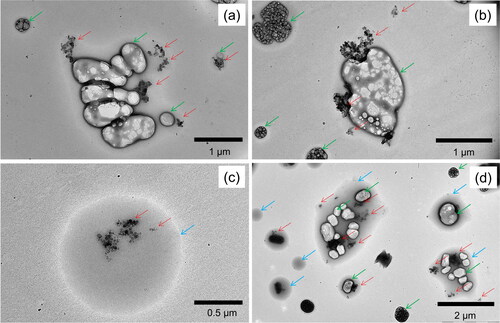
Figure 5. Typical examples of transmission electron microscope (TEM) images of ambient aerosols collected by an aerosol-impactor sampler installed on the research vessel SHINSEI MARU. Each panel shows samples collected around 12:00 local time on (a) July 27^th, (b) July 28^th, (c) July 30^th, and (d) August 1^st. Red arrows indicate individual BC aggregates, most of which were mixed with sulfate (green arrows) and/or organics (light blue arrows). The TEM images were obtained using a 120-kV TEM (JEM-1400, JEOL).

4. Results and discussion

4.1. The complex amplitude data

We only analyzed the s-channel data in this work as our laboratory test samples and atmospheric BC particles collected into water were mostly distributed in the submicron size domain and their S(0°)-distributions were hardly observed in the l-channel. For each sampled cohort, we discard the particle detection events with signal waveform width greater than its 50^th percentile value to increase the precision of the derived S(0°) data (Moteki 2021), with a resulting 50% reduction in the number of particles analyzed.

4.1.1. Laboratory test samples

Figure 6 shows a scatterplot of the S(0°) data points observed for each of the laboratory test samples dispersed in water. For the Fullerene soot and Vehicle exhaust particulates (Figure 6a and b), the linear-shape dense cluster of S(0°) data points with ImS(0°)/ReS(0°) ratio > ∼1 is attributable to BC aggregates with a high imaginary part of refractive index (Moteki 2020). For Fullerene soot, the sparse cluster of data points with ImS(0°)/ReS(0°) ratio < ∼0.5, which is attributable to non-absorbing particles, was excluded from the analyses. For Vehicle exhaust particulates, the curved-shape cluster of S(0°) data points with lower ImS(0°)/ReS(0°) ratio, which is attributable to water-insoluble refractory road dust particles (metallic oxides), was excluded from the analyses. For each of the Fullerene soot and Vehicle exhaust particulates, a principal curve fit was applied to the cluster of S(0°) data points of BC aggregates, and every 5^th percentile of the arclength coordinate s was selected to construct the input data vector for Bayesian inference (Figure 3).

Figure 6. Scatterplot of the complex forward-scattering amplitude obtained for each of the laboratory powder samples suspended in water. Black dots show raw single particle S(0°) data. The red-filled circles show the 0^th, 5^th, …, and 100^th percentiles of the arclength coordinate of the principal curve. These 21 data points were used as the observation data vector for Bayesian inference. The red circles are concentrated in proportion to the local density of raw data points.

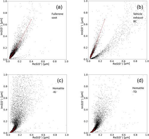
For each of the Hematite-KJ and Hematite-TD (Figure 6c and d), the clustered S(0°) data points distribute more broadly as |S(0°)| increased beyond ∼0.2 μm due to the pronounced effects of particle shape and orientation. The S(0°) distribution at |S(0°)| > ∼0.2 μm was appreciably broader in Hematite-KJ than in Hematite-TD, reflecting their morphological differences (c.f., Figure 4). For single-component but nonspherical particulate materials, the transition from tight to broad S(0°) cluster occurs when the particle size becomes large enough so that the mean internal field is quite sensitive to the details of the particle’s shape and orientation. The earlier transition to the broad cluster in Hematite-KJ around |S(0°)| ∼0.2 μm is likely due to its more sintered morphology and/or asymmetric envelope shape. In both Hematite-KJ and Hematite-TD, we only used S(0°) data points with |S(0°)| ≤ 0.15 μm for principal curve fit and following analyses to mitigate the potential bias of Bayesian inversion due to the shape model assumptions.

4.1.2. Atmospheric aerosol samples

Figure 7 shows the scatterplot of S(0°) data points of atmospheric water-insoluble aerosols on each observation day. In each of the 6 days, the linear-shape dense cluster of S(0°) data points with ImS(0°)/ReS(0°) ratio > ∼1 was distinguishable from other clusters with lower ImS(0°)/ReS(0°) ratios. We suppose the former cluster is solely attributable to BC aggregates for three reasons. Firstly, the S(0°) cluster was similar to those of laboratory BC materials. Secondly, the number concentration of aggregates of magnetite nanoparticles, which could exhibit S(0°) distributions indistinguishable from BC aggregates, was reported to be several orders of magnitude lower than the BC aggregates in the lower troposphere around East Asia (Moteki et al. 2017). Thirdly, other ubiquitous aerosol components that can form the linear-shape dense cluster of S(0°) data points with ImS(0°)/ReS(0°) ratio > ∼1 are not known.

Figure 7. Same plots as Figure 6 but for atmospheric water-insoluble aerosols collected into water on each of the 6 observation days. Principal curve fit was applied to the linear-shape cluster of data points with ImS(0°)/ReS(0°) > ∼1, which is attributable to BC aggregates.

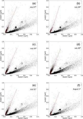
The distinct compact S(0°) clusters in each panel of Figure 7 are attributable to size-standard Polystyrene (PS) spheres with a refractive index of 1.585 + 0i. The PS particles attached to the inner surface of the aerosol-into-water collection system during the laboratory experiments (cf. Figure S4) were gradually detached during the observation. These S(0°) clusters were not observed in the purified water used for generating the steam jet of the collection system (i.e., blank samples).

A curved-shape dense S(0°) cluster with ImS(0°)/ReS(0°) ratio below the PS clusters was persistent throughout the 6 days (Figure 7). The water-insoluble non-BC materials responsible for this cluster were not investigated here. The clear separation between this non-BC $$ cluster and the BC cluster on the complex S(0°) plane suggests that the number fraction of BC-containing particles consisting of BC material and the non-BC water-insoluble materials was negligible as compared to the nearly pure particles of either class in the water medium. Otherwise, S(0°) data points with various ImS(0°)/ReS(0°) ratios between the two extremes, depending on the BC volume fraction of the internal mixture, would also have been frequently observed. This observational evidence supports the use of aggregate shape models without considering the internally mixed non-BC materials in our Bayesian inference of the refractive index of BC aggregates.

It was previously observed in the atmospheric boundary layer around this oceanic region that most of the submicron aerosol particles were comparably hygroscopic as ammonium sulfate (Mochida et al. 2011). It was reported that the hygroscopicity of the coating materials on the BC core was similar to that of the materials of BC-free submicron particles even in the less-aged urban plumes (Ohata et al. 2016). Therefore, it is no surprise if the coating materials on the BC core in our field observations were comparably hygroscopic with the ammonium sulfate and dissolved into the water through the aerosol-into-water collection procedure.

4.2. The refractive index

4.2.1. Laboratory test samples

Figure 8 shows the 90%, 50%, and 10% highest density credibility regions of the joint probability of (m_r, m_i) posterior pair obtained for each of the four laboratory test samples. The credibility region is displayed for each shape model assumption. Corresponding to Figures 8a–d, S6–S9 show computed chains of the posterior sample and its density distribution of each element of the parameter vector (${\overrightarrow{r}}_{\mathrm{v}},$ m_r, m_i, θ_s). The BB06-l and -h were also plotted in Figure 8 for comparison.

Figure 8. Posterior of real and imaginary parts of complex refractive index (m_r, m_i) for each laboratory sample derived from the data shown in Figure 6. (a) Fullerene soot, (b) Vehicle exhaust BC, (c) Hematite-KJ, (d) Hematite-TD. The three-level contour shows the 90%, 50%, and 10% highest density credibility regions for each of the AGGREGATE (green) and SPHPACK (blue) models. Marginalized density distributions of m_r and m_i are also shown along horizontal and vertical axes, respectively. In each panel, the BB06-l and -h values were also shown by gray-filled circles for comparison. In panels (a) and (b), the SPHPACK is more realistic shape model than the AGGREGATE for the reasons explained in the main text.

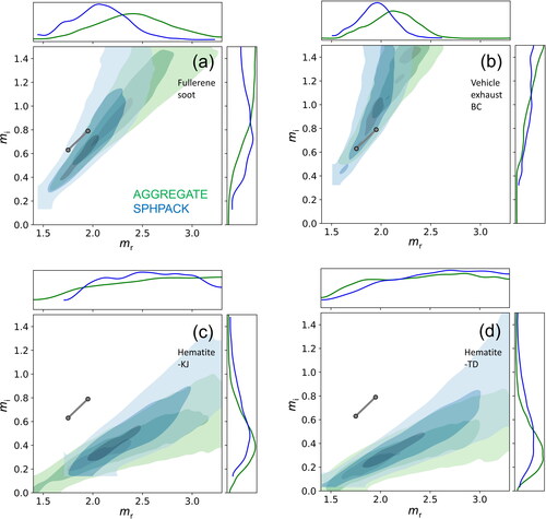
For both Fullerene soot and Vehicle exhaust BC, the shape parameter θ_s of the AGGREGATE model (fractal dimension) exhibited a skewed posterior distribution toward the upper boundary of the parameter domain [2.0, 2.5] (Figures S6 and S7), suggesting that the actual BC aggregates in these samples could be more compact than fractal-like aggregates with fractal dimension ∼2.5. By contrast, the shape parameter θ_s of the SPHPACK model (packing density) exhibited single modal posterior distributions within the parameter domain [0.05, 0.30] (Figures S6 and S7). This means that the SPHPACK model can reproduce the observed shape of the S(0°) cluster more confidently than the AGGREGATE model. The suitability of the SPHPACK model for these samples is also expected from the predominance of compact BC aggregates in their TEM images before dispersing into water (Figure 4). From this discussion, the credibility region of (m_r, m_i) for the SPHPACK model is more plausible than that of the AGGREGATE model. The (m_r, m_i) credibility region for the SPHPACK model was appreciably different between Vehicle exhaust BC and Fullerene soot, likely due to their difference in the degree of graphitization.

Hematite-KJ and Hematite-TD samples exhibited a much lower m_i/m_r ratio than the test BC samples. This contrast between hematite and BC is consistent with the difference in previously reported values of their refractive index (Schuster et al. 2016). The derived credibility regions of (m_r, m_i) were similar between Hematite-KJ and Hematite-TD despite their difference in particle morphology, as we had suppressed the sensitivity of inversion results to particle shape by using only small |S(0°)| data. As a result, the shape parameter θ_s was poorly constrained for these hematite samples (Figures S8 and S9).

Figure 9. Same plot as Figure 8 but for atmospheric BC results derived from the data shown in Figure 7. In each panel, the BB06-l and -h values were also shown by gray-filled circles for comparison. The dashed lines indicate the boundary of our suggested plausible (m_r, m_i) domain for atmospheric BC, which approximate the 90% highest density credibility regions. The SPHPACK is more realistic shape model than the AGGREGATE for the reasons explained in the main text.

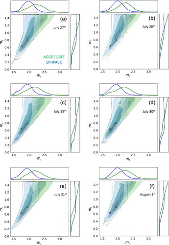
4.2.2. Atmospheric BC

Figures 9, S10–S15 show the same results as Figures 8, S6–S9 but for atmospheric BC aggregates collected into water. The credibility regions of (m_r, m_i) for atmospheric BC were closer to those of Vehicle exhaust BC rather than Fullerene soot. In any of the 6-day ambient BC samples, the shape parameter θ_s of the AGGREGATE model showed a skewed posterior distribution toward the upper boundary of the parameter domain, while that of the SPHPACK model showed a single modal distribution within the parameter domain (Figures S10–S15). These Bayesian inference results, as well as the predominance of relatively compact BC aggregate in TEM images of ambient aerosol samples before the collection into water (Figure 5), suggest that the SPHPACK is a more plausible shape model than the AGGREGATE. The posterior mode of packing density θ_s of the SPHPACK model was appreciably larger on the July 28^th sample (θ_s ∼ 0.2) than the July 27th, 29th–31th samples (θ_s∼0.15). According to the trajectories, July 28th data were predominantly influenced by the oceanic remote atmosphere around the western Pacific, whereas the July 27th and July 29th–31th data were more-or-less impacted by Japanese and/or continental emission sources. The larger packing density θ_s of BC aggregates on July 28^th is likely due to the further progression of aggregate compaction during their longer atmospheric residence times. Despite the systematic shift of shape parameter of BC aggregates on July 28^th, the 50% highest credibility region of (m_r, m_i) of BC aggregates on that day was not appreciably different from those of the other 5 days. This illustrates that our approach can suppress the bias of refractive index estimation due to the change in compactness of BC aggregates in the atmosphere. The 50% highest credibility region of (m_r, m_i) always contained the BB06-l and h values during the 6 days. The 50% highest credibility regions do not exclude the possibility of higher m_i values than BB06 for both Vehicle exhaust and atmospheric BC samples. As an approximation of the 90% highest credibility regions, we suggest a plausible (m_r, m_i) domain for atmospheric BC: (2) $$\{\begin{array}{l}\mathrm{m}\mathrm{ax}\left(0.27,\mathrm{ }1.1{7m}_{\mathrm{r}}-1.70\right)\le m_{\mathrm{i}}\le 2.50m_{\mathrm{r}}-3.50\text{ if }1.5\le m_{\mathrm{r}}\le 1.8,\\ 1.1{7m}_{\mathrm{r}}-1.70\le m_{\mathrm{i}}\le 1.50\text{ if }1.8\le m_{\mathrm{r}}\le 2.3,\end{array}\mathrm{ }$$(2) where the operator max(A, B) denotes the larger one of A and B. The boundary of the (m_r, m_i) domain defined by Equation (2)(2) $$\{\begin{array}{l}\mathrm{m}\mathrm{ax}\left(0.27,\mathrm{ }1.1{7m}_{\mathrm{r}}-1.70\right)\le m_{\mathrm{i}}\le 2.50m_{\mathrm{r}}-3.50\text{ if }1.5\le m_{\mathrm{r}}\le 1.8,\\ 1.1{7m}_{\mathrm{r}}-1.70\le m_{\mathrm{i}}\le 1.50\text{ if }1.8\le m_{\mathrm{r}}\le 2.3,\end{array}\mathrm{ }$$(2) was also shown in Figure 9.

Figure 10. Joint density plots of the posteriors of real and imaginary parts of refractive index, m_r, m_i, and the two volume-equivalent radii corresponding to the 95^th and 100^th percentiles of arclength coordinate of the principal curve, r_v95, r_v100 for atmospheric BC sampled on August 1^st. The three-level contour shows the 90%, 50%, and 10% highest density credibility regions in each of the AGGREGATE (green) and SPHPACK (blue) models. The SPHPACK is more realistic shape model than the AGGREGATE for the reasons explained in the main text.

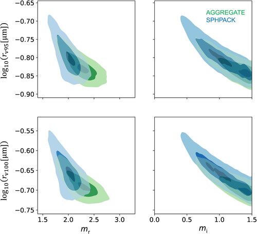
The inference uncertainty of the (m_r, m_i) of atmospheric BC collected into water, which was visualized as posterior distribution in Figure 9, is tightly correlated with the inference uncertainty of the volume-equivalent radii ${\overrightarrow{r}}_{\mathrm{v}},$ as illustrated in Figure 10. This suggests that the incorporation of an independently measured volume-equivalent size distribution of waterborne BC particles into the Bayesian inference procedure as additional data could help to reduce the inference uncertainty of the (m_r, m_i).

4.2.3. Another constraint from the reported mass absorption cross-sections

As shown in section 4.2.2, the actual amount of information contained in the S(0°) data was not enough to constrain the complex refractive index of BC aggregates to a fairly narrow (m_r, m_i) domain. In this section, we narrow down the plausible (m_r, m_i) domain for BC given by Equation (2)(2) $$\{\begin{array}{l}\mathrm{m}\mathrm{ax}\left(0.27,\mathrm{ }1.1{7m}_{\mathrm{r}}-1.70\right)\le m_{\mathrm{i}}\le 2.50m_{\mathrm{r}}-3.50\text{ if }1.5\le m_{\mathrm{r}}\le 1.8,\\ 1.1{7m}_{\mathrm{r}}-1.70\le m_{\mathrm{i}}\le 1.50\text{ if }1.8\le m_{\mathrm{r}}\le 2.3,\end{array}\mathrm{ }$$(2) by imposing another theoretical constraint. For this purpose, we use the reported MAC values for uncoated BC aggregates.

Liu et al. (2020) reviewed recent studies on direct measurements of MAC for several different types of flame-generated uncoated BC aerosols within ∼1 − 25 fg particle mass range (∼0.05 − 0.15 μm volume equivalent radius range, assuming 1.8 g cm⁻³ density). They summarized the reported MAC values as 8.0 ± 0.7 m² g⁻¹ at λ = 0.55 μm. We estimated the corresponding MAC value 7.0 ± 0.6 m² g⁻¹ at λ = 0.633 μm assuming the Absorption Ångström exponent = 1, which is a reasonable assumption for lacy flame-generated BC aggregates at visible wavelengths (Liu et al. 2020). To predict m = m_r + im_i values of BC aggregates theoretically consistent with a given MAC value, we adopted the corrected MAC formula according to the Rayleigh-Debye-Gans theory for Fractal Aggregate (RDGFA): (3) $${\mathrm{MAC}}_{\mathrm{RDGFAh}}=\frac{6\pi h}{\lambda {\rho }_{\mathrm{BC}}}\mathrm{I}\mathrm{m}\left(\frac{m^2-1}{m^2+2}\right),\mathrm{ }$$(3) where the ρ_BC is BC density which was assumed to be 1.8 g cm⁻³ (Liu et al. 2020), and the h is an empirical factor correcting the deviation from the theoretically exact MAC value predicted using rigorous light-scattering solvers for a cluster of spheres (e.g., superposition T-matrix methods). The h was reported to be within 0.9 − 1.3 for lacy BC aggregates with various monomer sizes, refractive indices, and shapes (Yon et al. 2008; Yon et al. 2014; Sorensen et al. 2018).

Figure 11 shows the (m_r, m_i) domain consistent with the parameter range 6.4 m² g⁻¹ ≤ MAC_RDGFAh ≤ 7.6 m² g⁻¹ and 0.9 ≤ h ≤ 1.3 calculated at λ = 0.633 μm according to Equation (3)(3) $${\mathrm{MAC}}_{\mathrm{RDGFAh}}=\frac{6\pi h}{\lambda {\rho }_{\mathrm{BC}}}\mathrm{I}\mathrm{m}\left(\frac{m^2-1}{m^2+2}\right),\mathrm{ }$$(3) . We regard this MAC-based (m_r, m_i) domain as another constraint on the plausible (m_r, m_i) domain of atmospheric BC, assuming the differences in (m_r, m_i) between atmospheric and flame-generated BCs were within the uncertainty range corresponding to the ranges in MAC_RDGFAh and h. The intersection of the S(0°)-based domain Equation (2)(2) $$\{\begin{array}{l}\mathrm{m}\mathrm{ax}\left(0.27,\mathrm{ }1.1{7m}_{\mathrm{r}}-1.70\right)\le m_{\mathrm{i}}\le 2.50m_{\mathrm{r}}-3.50\text{ if }1.5\le m_{\mathrm{r}}\le 1.8,\\ 1.1{7m}_{\mathrm{r}}-1.70\le m_{\mathrm{i}}\le 1.50\text{ if }1.8\le m_{\mathrm{r}}\le 2.3,\end{array}\mathrm{ }$$(2) and the MAC-based domain is approximately given by (4) $$\{\begin{array}{l}0.51+0.014m_{\mathrm{r}}^{5.2}\le m_{\mathrm{i}}\le 2.5m_{\mathrm{r}}-3.5\text{ if }1.7\le m_{\mathrm{r}}\le 1.8\\ 0.51+0.014m_{\mathrm{r}}^{5.2}\le m_{\mathrm{i}}\le 1.5\text{ if }1.8<m_{\mathrm{r}}\le 2.2\end{array}.\mathrm{ }$$(4)

Figure 11. Illustrating the three-different (m_r, m_i) domains for complex refractive index of BC: 1) a domain consistent with measured S(0°) for atmospheric BC (enclosed by black-dashed lines), 2) a domain consistent with measured MAC for various flame-generated BCs (red-filled area), and 3) a domain supported by both MAC- and S(0°)-measurements. The conventional assumptions BB06-l (1.75 + 0.63i) and -h (1.95 + 0.79i) (gray filled circles), and our recommendable value for practical uses 1.95 + 0.96i (blue-filled circle) are also plotted.

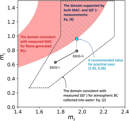
We suggest Equation (4)(4) $$\{\begin{array}{l}0.51+0.014m_{\mathrm{r}}^{5.2}\le m_{\mathrm{i}}\le 2.5m_{\mathrm{r}}-3.5\text{ if }1.7\le m_{\mathrm{r}}\le 1.8\\ 0.51+0.014m_{\mathrm{r}}^{5.2}\le m_{\mathrm{i}}\le 1.5\text{ if }1.8<m_{\mathrm{r}}\le 2.2\end{array}.\mathrm{ }$$(4) as a refined plausible (m_r, m_i) domain for atmospheric BC at λ = 0.633 μm, which is visualized as the hatched area in Figure 11.

Even though the BB06 values have been “accepted” in the climate and atmospheric science community since the publication of Bond and Bergstrom (2006) (cf. Table 1), they are located outside the plausible (m_r, m_i) domain Equation (4)(4) $$\{\begin{array}{l}0.51+0.014m_{\mathrm{r}}^{5.2}\le m_{\mathrm{i}}\le 2.5m_{\mathrm{r}}-3.5\text{ if }1.7\le m_{\mathrm{r}}\le 1.8\\ 0.51+0.014m_{\mathrm{r}}^{5.2}\le m_{\mathrm{i}}\le 1.5\text{ if }1.8<m_{\mathrm{r}}\le 2.2\end{array}.\mathrm{ }$$(4) . The persistent ∼30% underpredictions of MAC using the BB06-l or -h value, as pointed out by Liu et al. (2020), will be mitigated if its imaginary part is increased to a value inside the (m_r, m_i) domain Equation (4)(4) $$\{\begin{array}{l}0.51+0.014m_{\mathrm{r}}^{5.2}\le m_{\mathrm{i}}\le 2.5m_{\mathrm{r}}-3.5\text{ if }1.7\le m_{\mathrm{r}}\le 1.8\\ 0.51+0.014m_{\mathrm{r}}^{5.2}\le m_{\mathrm{i}}\le 1.5\text{ if }1.8<m_{\mathrm{r}}\le 2.2\end{array}.\mathrm{ }$$(4) .

4.2.4. A Recommended value for practical uses

For convenient uses of our final results (Equation (4)(4) $$\{\begin{array}{l}0.51+0.014m_{\mathrm{r}}^{5.2}\le m_{\mathrm{i}}\le 2.5m_{\mathrm{r}}-3.5\text{ if }1.7\le m_{\mathrm{r}}\le 1.8\\ 0.51+0.014m_{\mathrm{r}}^{5.2}\le m_{\mathrm{i}}\le 1.5\text{ if }1.8<m_{\mathrm{r}}\le 2.2\end{array}.\mathrm{ }$$(4) ) by climate and atmospheric researchers, we select a recommendable value from the (m_r, m_i) domain Equation (4)(4) $$\{\begin{array}{l}0.51+0.014m_{\mathrm{r}}^{5.2}\le m_{\mathrm{i}}\le 2.5m_{\mathrm{r}}-3.5\text{ if }1.7\le m_{\mathrm{r}}\le 1.8\\ 0.51+0.014m_{\mathrm{r}}^{5.2}\le m_{\mathrm{i}}\le 1.5\text{ if }1.8<m_{\mathrm{r}}\le 2.2\end{array}.\mathrm{ }$$(4) . We selected 1.95 + 0.96i, which was determined by increasing the imaginary part of the BB06-h to the lower m_i boundary of the plausible (m_r, m_i) domain Equation (4)(4) $$\{\begin{array}{l}0.51+0.014m_{\mathrm{r}}^{5.2}\le m_{\mathrm{i}}\le 2.5m_{\mathrm{r}}-3.5\text{ if }1.7\le m_{\mathrm{r}}\le 1.8\\ 0.51+0.014m_{\mathrm{r}}^{5.2}\le m_{\mathrm{i}}\le 1.5\text{ if }1.8<m_{\mathrm{r}}\le 2.2\end{array}.\mathrm{ }$$(4) . The selected 1.95 + 0.96i is fairly conservative in terms of our S(0°)-based observational evidence as it was always inside the 50% highest density credibility regions of Bayesian (m_r, m_i) posterior for atmospheric BC collected into water (Figure 9). Assuming the 1.95 + 0.96i instead of the BB06-h (1.95 + 0.79i) will result in a ∼16% increase of MAC for uncoated BC aggregates according to the RDGFA theory. Corresponding increases of calculated MAC for the BC aggregates coated by non-absorbing materials (e.g., sulfate, water) are expected to be similar magnitudes to the uncoated BC aggregates.

5. Conclusions

We provided a new observational constraint of the complex refractive index m = m_r + im_i of uncoated BC aggregates at visible wavelengths through single-particle measurements of complex forward-scattering amplitude S(0°) at λ = 0.633 μm. In our approach, the S(0°) measurement of water-insoluble aerosol particles in water successfully extracted the S(0°) data points attributable to pure BC aggregates avoiding the influences of other aerosol components. The simultaneous retrieval of particle shape information from the S(0°) data was shown to suppress the bias in inferred refractive index due to variability in the compactness of BC aggregates. The plausible (m_r, m_i) domain for atmospheric BC constrained from the S(0°)-based Bayesian inference was given by Equation (2)(2) $$\{\begin{array}{l}\mathrm{m}\mathrm{ax}\left(0.27,\mathrm{ }1.1{7m}_{\mathrm{r}}-1.70\right)\le m_{\mathrm{i}}\le 2.50m_{\mathrm{r}}-3.50\text{ if }1.5\le m_{\mathrm{r}}\le 1.8,\\ 1.1{7m}_{\mathrm{r}}-1.70\le m_{\mathrm{i}}\le 1.50\text{ if }1.8\le m_{\mathrm{r}}\le 2.3,\end{array}\mathrm{ }$$(2) . The (m_r, m_i) domain was narrowed down to Equation (4)(4) $$\{\begin{array}{l}0.51+0.014m_{\mathrm{r}}^{5.2}\le m_{\mathrm{i}}\le 2.5m_{\mathrm{r}}-3.5\text{ if }1.7\le m_{\mathrm{r}}\le 1.8\\ 0.51+0.014m_{\mathrm{r}}^{5.2}\le m_{\mathrm{i}}\le 1.5\text{ if }1.8<m_{\mathrm{r}}\le 2.2\end{array}.\mathrm{ }$$(4) by taking into account the consistency with recently reported MAC values for flame-generated BCs. From the constrained (m_r, m_i) domain Equation (4)(4) $$\{\begin{array}{l}0.51+0.014m_{\mathrm{r}}^{5.2}\le m_{\mathrm{i}}\le 2.5m_{\mathrm{r}}-3.5\text{ if }1.7\le m_{\mathrm{r}}\le 1.8\\ 0.51+0.014m_{\mathrm{r}}^{5.2}\le m_{\mathrm{i}}\le 1.5\text{ if }1.8<m_{\mathrm{r}}\le 2.2\end{array}.\mathrm{ }$$(4) , we suggest 1.95 + 0.96i as a recommendable assumption of m_r + im_i for uncoated BC aggregates in the atmosphere at visible wavelengths, whose imaginary part is 0.17 larger than that of the current “accepted” assumption BB06-h (1.95 + 0.79i). We briefly estimated that an update of the BC refractive index assumption from the conventional 1.95 + 0.79i to the suggested 1.95 + 0.96i results in a ∼16% increase of calculated light absorptions by pure BC and BC-containing aerosols. Instead of the BB06-h, we recommend using the 1.95 + 0.96i for climate modeling and remote sensing as it is more consistent with recent direct measurements of S(0°) and MAC.

Author contributions

NM designed the research, developed the instruments and codes, and performed the calculations and data analyses. SO and AY operated instruments during the research cruise. KA performed TEM analyses of particle samples.

Sample availability

Samples used for this study (Fullerene soot, Vehicle Exhaust Particulates, Hematite-KJ, Hematite-TD) are available from the corresponding author upon reasonable request.

Acknowledgments

We thank the Drs. Y. Kawai, M. Koike, T. Miyakawa, and JAMSTEC staff for supporting the atmospheric aerosol measurements using the research vessel SHINSEI MARU. The authors thank J. P. Schwarz and A. Khalizov for providing insightful comments. The authors thank D. W. Mackowski for providing the MSTM code used in this publication. The authors thank S. Zhang for providing the “pcurvepy” Python module for principal curve fit. The authors thank the NOAA Air Resources Laboratory (ARL) for providing the HYSPLIT transport and dispersion model and/or READY website (https://www.ready.noaa.gov) used in this publication.

Disclosure statement

The contact author has declared that none of the authors have competing interests.

Code availability

The originally developed Python module used for auto-differentiable multidimensional spline interpolation of gridded data is available from: https://github.com/nmoteki/ndimsplinejax. The code used for generating fractal-like aggregates of spheres is available from https://github.com/nmoteki/aggregate_generator. Other codes used for this study are available from the corresponding author upon reasonable request.

Data availability statement

Data generated for Figures 6 and 7 are available from: https://doi.org/10.5281/zenodo.7478889.

Additional information

Funding

Funds were provided by the Environment Research and Technology Development Fund (JPMEERF20202003) of the Environmental Restoration and Conservation Agency, the Japan Society for the Promotion of Science (JSPS) KAKENHI program (JP19H04236, JP19KK0289, JP19H04259, JP19H05699, 22H03722, and 22H01294), and the Arctic Challenge for Sustainability ArCS II project (JPMXD1420318865) of the Ministry of Education, Culture, Sports, Science, and Technology (MEXT) of Japan.

References

- Adachi, K., N. Oshima, S. Ohata, A. Yoshida, N. Moteki, and M. Koike. 2021. Compositions and mixing states of aerosol particles by aircraft observations in the Arctic springtime, 2018. Atmos. Chem. Phys. 21 (5):3607–26. doi:10.5194/acp-21-3607-2021.
- Adachi, K., Y. Zaizen, M. Kajino, and Y. Igarashi. 2014. Mixing state of regionally transported soot particles and the coating effect on their size and shape at a mountain site in Japan. J. Geophys. Res. Atmos. 119 (9):5386–96. doi:10.1002/2013JD020880.
- Baumgardner, D., O. Popovicheva, J. Allan, V. Bernardoni, J. Cao, F. Cavalli, J. Cozic, E. Diapouli, K. Eleftheriadis, P. J. Genberg, et al. 2012. Soot reference materials for instrument calibration and intercomparisons: A workshop summary with recommendations. Atmos. Meas. Tech. 5 (8):1869–87. doi:10.5194/amt-5-1869-2012.
- Beeler, P., and R. K. Chakrabarty. 2022. Constraining the particle-scale diversity of black carbon light absorption using a unified framework. Atmos. Chem. Phys. 22 (22):14825–36. doi:10.5194/acp-22-14825-2022.
- Bhandari, J., S. China, K. K. Chandrakar, G. Kinney, W. Cantrell, R. A. Shaw, L. R. Mazzoleni, G. Girotto, N. Sharma, K. Gorkowski, et al. 2019. Extensive soot compaction by cloud processing from laboratory and field observations. Sci. Rep. 9 (1):11824. doi:10.1038/s41598-019-48143-y.
- Bond, T. C., and R. W. Bergstrom. 2006. Light absorption by carbonaceous particles: An investigative review. Aerosol Sci. Technol. 40 (1):27–67. doi:10.1080/02786820500421521.
- Bond, T. C., S. J. Doherty, D. W. Fahey, P. M. Forster, T. Berntsen, B. J. DeAngelo, M. G. Flanner, S. Ghan, B. Kärcher, D. Koch, et al. 2013. Bounding the role of black carbon in the climate system: A scientific assessment. J. Geophys. Res. Atmos. 118 (11):5380–552. doi:10.1002/jgrd.50171.
- Brown, H., X. Liu, R. Pokhrel, S. Murphy, Z. Lu, R. Saleh, T. Mielonen, H. Kokkola, T. Bergman, G. Myhre, et al. 2021. Biomass burning aerosols in most climate models are too absorbing. Nat. Commun. 12 (1):277. doi:10.1038/s41467-020-20482-9.
- Buseck, P. R., K. Adachi, A. Gelencsér, É. Tompa, and M. Pósfai. 2014. Ns-soot: A material-based term for strongly light-absorbing carbonaceous particles. Aerosol Sci. Technol. 48 (7):777–88. doi:10.1080/02786826.2014.919374.
- Chang, H. C., and T. T. Charalampopoulos. 1990. Determination of the wavelength dependence of refractive indices of flame soot. Proc. R. Soc. Lond. A. Math. Phys. Sci. 430 (1880):577–91. doi:10.1098/rspa.1990.0107.
- Cheng, T., X. Gu, Y. Wu, H. Chen, and T. Yu. 2013. The optical properties of absorbing aerosols with fractal soot aggregates: Implications for aerosol remote sensing. J. Quant. Spectrosc. Radiat. Transf. 125:93–104. doi:10.1016/j.jqsrt.2013.03.012.
- Corbin, J. C., H. Czech, D. Massabò, F. B. de Mongeot, G. Jakobi, F. Liu, P. Lobo, C. Mennucci, A. A. Mensah, J. Orasche, et al. 2019. Infrared-absorbing carbonaceous tar can dominate light absorption by marine-engine exhaust. npj Clim. Atmos. Sci. 2 (1):1–10. doi:10.1038/s41612-019-0069-5.
- Corbin, J. C., R. L. Modini, and M. Gysel-Beer. 2023. Mechanisms of soot-aggregate restructuring and compaction. Aerosol Sci. Technol. 57 (2):89–111. doi:10.1080/02786826.2022.2137385.
- Giglio, M., and M. A. C. Potenza. 2011. Method of measuring properties of particles and corresponding apparatus. US Patent 7924431B2, issued April 12, 2011.
- Hastie, T., and W. Stuetzle. 1989. Principal curves. J. Am. Stat. Assoc. 84 (406):502–16. doi:10.2307/2289936.
- Hastings, W. K. 1970. Monte Carlo sampling methods using Markov chains and their applications. Biometrika 57 (1):97–109. doi:10.1093/biomet/57.1.97.
- Hess, M., P. Koepke, and I. Schult. 1998. Optical properties of aerosols and clouds: The software package OPAC. Bull. Amer. Meteor. Soc. 79 (5):831–44. doi:10.1175/1520-0477(1998)079 < 0831:OPOAAC>2.0.CO;2.
- Hoffman, M. D., and A. Gelman. 2014. The No-U-Turn sampler: Adaptively setting path lengths in Hamiltonian Monte Carlo. J. Mach. Learn. Res. 15 (1):1593–623.
- Honda, M. 2021. Multielement quantification and Pb isotope analysis of the certified reference material ERM-CZ120 for fine particulate matter. Geochem. J. 55 (6):355–71. doi:10.2343/geochemj.2.0642.
- Kahnert, M., and A. Devasthale. 2011. Black carbon fractal morphology and short-wave radiative impact: A modelling study. Atmos. Chem. Phys. 11 (22):11745–59. doi:10.5194/acp-11-11745-2011.
- Koike, M., N. Moteki, P. Khatri, T. Takamura, N. Takegawa, Y. Kondo, H. Hashioka, H. Matsui, A. Shimizu, and N. Sugimoto. 2014. Case study of absorption aerosol optical depth closure of black carbon over the East China Sea. J. Geophys. Res. Atmos. 119 (1):122–36. doi:10.1002/2013JD020163.
- Laborde, M., P. Mertes, P. Zieger, J. Dommen, U. Baltensperger, and M. Gysel. 2012. Sensitivity of the single particle soot photometer to different black carbon types. Atmos. Meas. Tech. 5 (5):1031–43. doi:10.5194/amt-5-1031-2012.
- Li, L., O. Dubovik, Y. Derimian, G. L. Schuster, T. Lapyonok, P. Litvinov, F. Ducos, D. Fuertes, C. Chen, Z. Li, et al. 2019. Retrieval of aerosol components directly from satellite and ground-based measurements. Atmos. Chem. Phys. 19 (21):13409–43. doi:10.5194/acp-19-13409-2019.
- Liu, F., J. Yon, A. Fuentes, P. Lobo, G. J. Smallwood, and J. C. Corbin. 2020. Review of recent literature on the light absorption properties of black carbon: Refractive index, mass absorption cross section, and absorption function. Aerosol Sci. Technol. 54 (1):33–51. doi:10.1080/02786826.2019.1676878.
- Liu, L., and M. I. Mishchenko. 2005. Effects of aggregation on scattering and radiative properties of soot aerosols. J. Geophys. Res. 110 (D11):D11211. doi:10.1029/2004JD005649.
- Mackowski, D. W. 2008. Exact solution for the scattering and absorption properties of sphere clusters on a plane surface. J. Quant. Spectrosc. Radiat. Transf. 109 (5):770–88. doi:10.1016/j.jqsrt.2007.08.024.
- Mackowski, D. W., and M. I. Mishchenko. 2011. A multiple sphere T-matrix Fortran code for use on parallel computer clusters. J. Quant. Spectrosc. Radiat. Transf. 112 (13):2182–92. doi:10.1016/j.jqsrt.2011.02.019.
- Moosmüller, H., R. K. Chakrabarty, and W. P. Arnott. 2009. Aerosol light absorption and its measurement: A review. J. Quant. Spectrosc. Radiat. Transf. 110 (11):844–78. doi:10.1016/j.jqsrt.2009.02.035.
- Mochida, M., C. Nishita‐Hara, H. Furutani, Y. Miyazaki, J. Jung, K. Kawamura, and M. Uematsu. 2011. Hygroscopicity and cloud condensation nucleus activity of marine aerosol particles over the western North Pacific. J. Geophys. Res. 116 (D6):D06204. doi:10.1029/2010JD014759.
- Moteki, N. 2020. Capabilities and limitations of the single-particle extinction and scattering method for estimating the complex refractive index and size-distribution of spherical and non-spherical submicron particles. J. Quant. Spectrosc. Radiat. Transf. 243:106811. doi:10.1016/j.jqsrt.2019.106811.
- Moteki, N. 2021. Measuring the complex forward-scattering amplitude of single particles by self-reference interferometry: CAS-v1 protocol. Opt. Express. 29 (13):20688–714. doi:10.1364/OE.423175.
- Moteki, N., and Y. Kondo. 2010. Dependence of laser-induced incandescence on physical properties of black carbon aerosols: Measurements and theoretical interpretation. Aerosol Sci. Technol. 44 (8):663–75. doi:10.1080/02786826.2010.484450.
- Moteki, N., K. Adachi, S. Ohata, A. Yoshida, T. Harigaya, M. Koike, and Y. Kondo. 2017. Anthropogenic iron oxide aerosols enhance atmospheric heating. Nat. Commun. 8:15329. doi:10.1038/ncomms15329.
- Ohata, S., J. P. Schwarz, N. Moteki, M. Koike, A. Takami, and Y. Kondo. 2016. Hygroscopicity of materials internally mixed with black carbon measured in Tokyo. J. Geophys. Res. Atmos. 121 (1):362–81. doi:10.1002/2015JD024153.
- Oshima, N., S. Yukimoto, M. Deushi, T. Koshiro, H. Kawai, T. Y. Tanaka, and K. Yoshida. 2020. Global and Arctic effective radiative forcing of anthropogenic gases and aerosols in MRI-ESM2.0. Prog. Earth Planet. Sci. 7:38. doi:10.1186/s40645-020-00348-w.
- Phan, D., N. Pradhan, and M. Jankowiak. 2019. Composable effects for flexible and accelerated probabilistic programming in NumPyro. arXiv preprint. arXiv:1912.11554 doi:10.48550/arXiv.1912.11554.
- Potenza, M. A., T. Sanvito, and A. Pullia. 2015. Measuring the complex field scattered by single submicron particles. AIP Adv. 5 (11):117222. doi:10.1063/1.4935927.
- Potenza, M. A. C., Ž. Krpetić, T. Sanvito, Q. Cai, M. Monopoli, J. M. De Araujo, C. Cella, L. Boselli, V. Castagnola, P. Milani, et al. 2017. Detecting the shape of anisotropic gold nanoparticles in dispersion with single particle extinction and scattering. Nanoscale 9 (8):2778–84. doi:10.1039/C6NR08977A.
- Qin, Z., Q. Zhang, J. Luo, and Y. Zhang. 2022. Optical properties of soot aggregates with different monomer shapes. Environ. Res. 214 (Pt 2):113895. doi:10.1016/j.envres.2022.113895.
- Ramezanpour, B., and D. W. Mackowski. 2019. Direct prediction of bidirectional reflectance by dense particulate deposits. J. Quant. Spectrosc. Radiat. Transf. 224:537–49. doi:10.1016/j.jqsrt.2018.12.012.
- Rolph, G., A. Stein, and B. Stunder. 2017. Real-time environmental applications and display system: Ready. Environ. Model. Softw. 95:210–28. doi:10.1016/j.envsoft.2017.06.025.
- Samset, B. H. 2022. Aerosol absorption has an underappreciated role in historical precipitation change. Commun. Earth Environ. 3 (1):242. doi:10.1038/s43247-022-00576-6.
- Samset, B. H., C. W. Stjern, E. Andrews, R. A. Kahn, G. Myhre, M. Schulz, and G. L. Schuster. 2018. Aerosol absorption: Progress towards global and regional constraints. Curr. Clim. Change Rep. 4 (2):65–83. doi:10.1007/s40641-018-0091-4.
- Sand, M., B. H. Samset, G. Myhre, J. Gliß, S. E. Bauer, H. Bian, M. Chin, R. Checa-Garcia, P. Ginoux, Z. Kipling, et al. 2021. Aerosol absorption in global models from AeroCom phase III. Atmos. Chem. Phys. 21 (20):15929–47. doi:10.5194/acp-21-15929-2021.
- Scarnato, B. V., S. Vahidinia, D. T. Richard, and T. W. Kirchstetter. 2013. Effects of internal mixing and aggregate morphology on optical properties of black carbon using a discrete dipole approximation model. Atmos. Chem. Phys. 13 (10):5089–101. doi:10.5194/acp-13-5089-2013.
- Scarnato, B. V., S. China, K. Nielsen, and C. Mazzoleni. 2015. Perturbations of the optical properties of mineral dust particles by mixing with black carbon: A numerical simulation study. Atmos. Chem. Phys. 15 (12):6913–28. doi:10.5194/acp-15-6913-2015.
- Schuster, G. L., O. Dubovik, and A. Arola. 2016. Remote sensing of soot carbon–Part 1: Distinguishing different absorbing aerosol species. Atmos. Chem. Phys. 16 (3):1565–85. doi:10.5194/acp-16-1565-2016.
- Slowik, J. G., E. S. Cross, J. H. Han, P. Davidovits, T. B. Onasch, J. T. Jayne, L. R. Williams, M. R. Canagaratna, M. R. Worsnop, D. R. Chakrabarty, et al. 2007. An inter-comparison of instruments measuring black carbon content of soot particles. Aerosol Sci. Technol. 41 (3):295–314. doi:10.1080/02786820701197078.
- Sorensen, C. M., J. Yon, F. Liu, J. Maughan, W. R. Heinson, and M. J. Berg. 2018. Light scattering and absorption by fractal aggregates including soot. J. Quant. Spectrosc. Radiat. Transf. 217:459–73. doi:10.1016/j.jqsrt.2018.05.016.
- Stagg, B. J., and T. T. Charalampopoulos. 1993. Refractive indices of pyrolytic graphite, amorphous carbon, and flame soot in the temperature range 25 to 600 C. Combust. Flame 94 (4):381–96. doi:10.1016/0010-2180(93)90121-I.
- Stein, A. F., R. R. Draxler, G. D. Rolph, B. J. B. Stunder, M. D. Cohen, and F. Ngan. 2015. NOAA's HYSPLIT atmospheric transport and dispersion modeling system. Bull. Am. Meteor. Soc. 96 (12):2059–77. doi:10.1175/BAMS-D-14-00110.1.
- Stier, P., J. H. Seinfeld, S. Kinne, and O. Boucher. 2007. Aerosol absorption and radiative forcing. Atmos. Chem. Phys. 7 (19):5237–61. doi:10.5194/acp-7-5237-2007.
- Wang, Y., F. Liu, C. He, L. Bi, T. Cheng, Z. Wang, H. Zhang, X. Zhang, Z. Shi, and W. Li. 2017. Fractal dimensions and mixing structures of soot particles during atmospheric processing. Environ. Sci. Technol. Lett. 4 (11):487–93. doi:10.1021/acs.estlett.7b00418.
- Wu, Y., T. Cheng, L. Zheng, and H. Chen. 2015. A study of optical properties of soot aggregates composed of poly-disperse monomers using the superposition T-matrix method. Aerosol Sci. Technol. 49 (10):941–9. doi:10.1080/02786826.2015.1083938.
- Wu, Y., T. Cheng, D. Liu, J. D. Allan, L. Zheng, and H. Chen. 2018. Light absorption enhancement of black carbon aerosol constrained by particle morphology. Environ. Sci. Technol. 52 (12):6912–9. doi:10.1021/acs.est.8b00636.
- Yon, J., C. Roze, T. Girasole, A. Coppalle, and L. Mees. 2008. Extension of RDG-FA for scattering prediction of aggregates of soot taking into account interactions of large monomers. Part. Part. Syst. Charact. 25 (1):54–67. doi:10.1002/ppsc.200700011.
- Yon, J., F. Liu, A. Bescond, C. Caumont-Prim, C. Roze, F.- X. Ouf, and A. Coppalle. 2014. Effects of multiple scattering on radiative properties of soot fractal aggregates. J. Quant. Spectrosc. Radiat. Transf. 133:374–81. doi:10.1016/j.jqsrt.2013.08.022.
- Yoshida, A., N. Moteki, and K. Adachi. 2022. Identification and particle sizing of submicron mineral dust by using complex forward-scattering amplitude data. Aerosol Sci. Technol. 56 (7):609–22. doi:10.1080/02786826.2022.2057839.
- Yu, F., G. Luo, and X. Ma. 2012. Regional and global modeling of aerosol optical properties with a size, composition, and mixing state resolved particle microphysics model. Atmos. Chem. Phys. 12 (13):5719–36. doi:10.5194/acp-12-5719-2012.
- Zaveri, R. A., J. C. Barnard, R. C. Easter, N. Riemer, and M. West. 2010. Particle‐resolved simulation of aerosol size, composition, mixing state, and the associated optical and cloud condensation nuclei activation properties in an evolving urban plume. J. Geophys. Res. 115 (D17):D17210. doi:10.1029/2009JD013616.