The volatility of pollen extracts and their main constituents in aerosolized form via the integrated volume method (IVM) and the volatility basis set (VBS)

Abstract

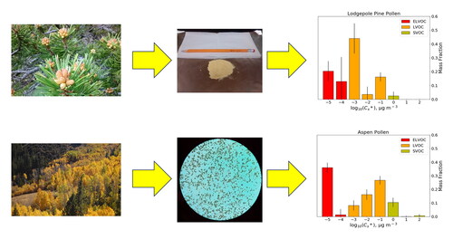
The volatility of organic aerosol in the atmosphere is an important quality that determines the aerosol/gas partitioning of compounds in the atmosphere and thus influences their ability to participate in gas-phase reactions in the atmosphere. In this research, the volatility of biological aerosols, specifically water-soluble pollen extracts and their chemical constituents, are studied for important thermodynamic properties such as saturation vapor concentration and latent heat of vaporization. The integrated volume method (IVM) was applied to characterize these properties for various free amino acids and saccharides in pollen, and the volatility basis set (VBS) approach was utilized to obtain a distribution of the mass fraction of pollen extracts with respect to saturation vapor concentration. Our results indicate that among seven compounds tested with the IVM, proline, γ-aminobutyric acid, and fructose had semivolatile saturation vapor concentrations of 17.5 ± 2.2, 14.7 ± 0.8, and 4.4 ± 0.5 μg m⁻³, respectively. Additionally, our VBS measurements indicate that aspen pollen extract contains a greater semivolatile mass fraction (up to 8.5% of total water-soluble mass) than lodgepole pine pollen (up to 2.2%), indicating that different pollen species may contribute to the total atmospheric semivolatile organic compound (SVOC) and low volatile organic compound (LVOC) budgets differently. Depending on estimates of several factors, fluxes and concentrations of SVOCs and LVOCs from pollen could be comparable to other sources such as biomass burning and ambient urban emissions, though further research is needed to better constrain the contribution of pollen and other bioaerosols to organic compounds in the atmosphere.

Graphical abstract

EDITOR:

• Cari Dutcher

1. Introduction

Biological aerosols, also referred to as bioaerosols, are any aerosol in the atmosphere that is biological in origin. Appearing in the atmosphere in sizes ranging from nanometers to several hundred micrometers in diameter, common examples of bioaerosols include viruses, bacteria, fungal spores, pollen, algae, as well as biological molecules such as proteins, lipids, and saccharides (Axelrod, Samburova, and Khlystov 2021; Fröhlich-Nowoisky et al. 2016). In recent years, bioaerosols have become a topic of increasingly intense research due to the current lack of knowledge on their chemistry, biological properties, and impact on the environment, and because research so far indicates that these aerosols may play a major role in cloud/ice nucleation, geochemical cycles, agriculture, and human health (Andreae and Rosenfeld 2008; Després et al. 2012; Kim, Kabir, and Jahan 2018).

Among the most common bioaerosols in the atmosphere is pollen, the male reproductive unit of most plants (Bedinger 1992). Pollen is especially known for causing seasonal allergies in humans that cost billions USD per year globally and is expected to increase with the effects of climate change in the future (D’Amato et al. 2020; Schaffner et al. 2020). It is also known for acting as ice nuclei and cloud condensation nuclei (Fröhlich-Nowoisky et al. 2016; Pope 2010; Steiner et al. 2015). In addition, certain species of pollen grains (e.g., birch pollen, elm pollen, various grass pollens) have been known to rupture in high-humidity conditions and form subpollen particles (SPPs) (Hughes et al. 2020; Miguel et al. 2006; Steiner et al. 2015). Due to this rupturing behavior, it is surmised that chemical constituents typically housed within the pollen grain may be exposed in the atmosphere, and as such, it is important to study how chemical constituents within pollen behave physically and chemically in the atmosphere.

An important physical property of aerosolized pollen and pollen constituents that is the central focus of this study is volatility - the tendency for compounds to evaporate to the gas phase at atmospherically-relevant temperatures and pressures. Two key parameters in defining the volatility of a compound are saturation vapor pressure (P_sat) and latent heat of vaporization and/or sublimation (ΔH). Saturation vapor pressure is defined as the vapor pressure of a pure compound in equilibrium (no net evaporation or condensation) with its condensed phase in a closed system at a given temperature. Under equal conditions (e.g., equal concentration in the particle phase, activity, and mixing state), compounds with a greater saturation vapor pressure will be present in larger quantities in the gas phase than those having lower saturation vapor pressure. In terms of aerosol load in the atmosphere, a more commonly used form of the P_sat parameter is saturation vapor concentration (C_sat), or the mass per unit volume of a gaseous compound that exists in equilibrium with its condensed phase (aerosol). Latent heat (enthalpy) of vaporization is the amount of energy required for a mole of a substance to change from liquid phase to gas phase (or from solid phase to gas phase, called the latent heat of sublimation), and higher values indicate that the saturation vapor concentration of the compound will have a greater dependence on temperature (Donahue et al. 2006).

In the atmosphere, an organic compound is considered a volatile organic compound (VOC) when its saturation vapor concentration at the standard temperature and pressure (STP) is 3 x 10⁶ μg m⁻³ or greater, intermediate-volatile (IVOC) for saturation vapor concentrations between 3 × 10⁶ and 3 × 10² μg m⁻³, semi-volatile (SVOC) for saturation vapor concentration between 3 × 10² and 3 × 10⁻¹ μg m⁻³, low-volatile (LVOC) for saturation vapor concentrations between 3 × 10⁻¹ and 3 × 10⁻⁴ μg m⁻³, and extremely low-volatile (ELVOC) when its saturation vapor concentration is 3 × 10⁻⁴ μg m⁻³ or less (Donahue, Kroll, et al. 2012). The volatility and chemical reactivity of compounds determines the degree to which they participate in gas-phase chemistry in the atmosphere, and thus their potential to react and produce secondary organic aerosol (SOA), as gas-phase reaction rates are often higher than heterogeneous (i.e., occurring on a particle surface) reaction rates (Cao et al. 2018; Robinson et al. 2007; Saleh, Shihadeh, and Khlystov 2009). While some biogenic volatile organic compounds (BVOCs) such as isoprene and α-pinene are well-studied (Kavouras, Mihalopoulos, and Stephanou 1998; Li et al. 2019), due to their high volatility and high emission rates in the atmosphere (Laothawornkitkul et al. 2009; McGenity, Crombie, and Murrell 2018; Pacifico et al. 2009; Peñuelas and Staudt 2010), oxidation of intermediate and semi-volatile organic compounds has also been shown to contribute significantly to the total SOA budget (Robinson et al. 2007) and are being studied at an increasing frequency in the past decade. Furthermore, due to the fact that bioaerosols are emitted in amounts of anywhere between 10 and 1000 Tg yr⁻¹ (the estimates vary widely due to high variability in release, and difficulty in measurement) (Després et al. 2012), even low volatile bioaerosol constituents may still evaporate in appreciable quantities and participate in gas-phase chemistry. As such, characterizing the volatility properties of these compounds is very important. However, volatility properties of bioaerosols and common bioaerosol constituents (potentially released via grain rupture and SPP formation) in the atmosphere are not well studied. The degree to which these molecules become oxidized in the atmosphere is not well-known, and the understanding of how they may cause SOA formation is still incomplete (Estillore, Trueblood, and Grassian 2016). This research focuses on the volatility amino acids and saccharides, as they are shown to be major fractions of the water-soluble mass of several species of pollen (Axelrod, Samburova, and Khlystov 2021). It should be noted that these compounds can also be emitted into the atmosphere via biomass burning, agricultural activities, and soil resuspension (Song et al. 2017; Vincenti et al. 2022; Zhu et al. 2020), furthering the importance of studying their volatility.

Due to analytical and experimental difficulties involved with measuring the evaporation behavior of semi-and low-volatile compounds, numerical models (such as the ones used by the Environmental Protection Agency’s Estimation Programs Interface suite; Card et al. 2017) utilize functional group information (group contribution methods) to estimate the saturation vapor pressure and latent heat of phase change of chemical compounds (e.g., modified Mackay or Grain-Watson methods) (Barley and McFiggans 2010). However, these numerical models often utilize assumptions for melting and boiling points and critical temperature and pressure (Komkoua Mbienda et al. 2013) and tend to deviate from one another, and often do not claim high accuracy for compounds of low vapor pressures (e.g., <100 Pa). Additionally, these models are known for being inaccurate with compounds that have a high number of different types of functional groups (Barley and McFiggans 2010). Furthermore, while latent heats of sublimation of compounds have been estimated using group contribution methods (e.g., amino acids) (Sagadeev, Gimadeev, and Barabanov 2010), saturation vapor pressures are often not modeled in unison.

The purpose of this research is to gain insight into the volatility properties of bioaerosols by direct measurements of the saturation vapor concentrations and latent heats of vaporization of several main pollen constituents (amino acids and saccharides), as well as of the volatility basis set (VBS) (Donahue et al. 2006) of pollen extract of two tree species, aspen (Populus tremuloides) and lodgepole pine (Pinus contorta). To our knowledge, this is the first study that attempts to determine these parameters for these compounds in aerosolized form, and the first study to perform an analysis of volatility of pollen extracts.

2. Methods

2.1. Aerosol sample preparation

In all experiments, aerosols were generated from solution dissolved in ultra-high purity (UHP) deionized water (Elga-Veolia PURELAB Chorus, UK). The pure compounds of sucrose, glucose, fructose, γ-aminobutyric acid (GABA), asparagine, leucine, and proline (Sigma Aldrich, Burlington, MA, USA) were each prepared in 0.01% concentrations at room temperature and used in the IVM experimental setup (section 2.2.1) immediately after preparation.

Lodgepole pine pollen was collected directly from the male cones of pollinating trees during the 2021 pollen season (April-June) in the area surrounding Reno, NV and Lake Tahoe, USA. Following collection, pollen was filtered through a 0.25 mm stainless steel mesh to remove larger non-pollen plant particles, and then the mesh-filtered pollen was weighed and mixed with UHP water at a 2%-weight concentration in Bertin Minilys lysing vials before being run on the Bertin Minilys tissue homogenizer (Rockville, MD, USA) to physically break apart the pollen grains (simulating SPP formation and pollen constituent release in water in the atmosphere). The solution was then centrifuged, and the supernatant was collected and 2x-diluted (effectively a 1.0% dry weight solution) and filtered through 0.45 μm pore size hydrophilic polytetrafluoroethylene (PTFE) syringe filters (Foxx Life Sciences, Salem, NH, USA). The filtered extract was then used immediately in the TDMA experimental setup (section 2.2.2). For aspen pollen extract, the preparation was the same as lodgepole pine pollen, except the pollen was purchased from Sigma-Aldrich.

2.2. Volatility measurements

In our experiments, the aerosol volatility was characterized using two thermodenuder-based methods. Namely, the integrated volume method (IVM) was used to characterize single component aerosols, while the tandem differential mobility analyzer (TDMA) method was used to characterize the volatility of pollen extracts. Both methods have been used to characterize volatility of various compounds and compound mixtures (Bilde et al. 2015). The IVM operates by equilibrating the aerosol at different temperatures and thus does not require assumptions regarding various aerosol properties such as the surface tension and the evaporation coefficient (Saleh, Walker, and Khlystov 2008). At the same time, it is very difficult to separate these parameters from the measured saturation concentration using the TDMA method (Saleh, Shihadeh, and Khlystov 2009), such that TDMA studies have to assume at least the value of the evaporation coefficient, which is generally taken to be 1 (e.g., Bilde et al. 2003; Tao and Mcmurry 1989). To avoid large uncertainties associated with assuming the evaporation coefficient, the IVM was used to study the single component aerosols. The IVM, however, is not easily applied to measure the saturation vapor concentrations of multi-component aerosol because the equilibrated partitioning of individual compounds depends on the equilibrated total organic aerosol concentration of the entire multi-component mixture. Therefore, in this study, the TDMA was used for volatility measurements of the pollen extract aerosols. Both methods are briefly described in separate sections below.

It should be also noted that thermodenuder techniques require working at elevated temperatures, which might lead to thermal decomposition of the aerosol compounds prior to their evaporation to the gas phase. For this reason, care was taken to limit the working temperature range to be below temperature ranges reported for observed thermal decomposition of these compounds in previous works (Jirasatid and Nopharatana 2021; Li et al. 2006; Moldoveanu 2019; Schaberg, Wroblowski, and Goertz 2018; Weiss et al. 2018) except in the case of sucrose, as will be discussed in the Results section. Temperature ranges used in our experiments are given in Table S1.

2.2.1. The integrated volume method

The IVM method was demonstrated to be comparable to other methods used for measurements of aerosol volatility (Bilde et al. 2015). It is discussed in detail elsewhere (Saleh, Walker, and Khlystov 2008) and only a brief summary is given here. The IVM is based on measuring the difference in gas-particle equilibrated aerosol volume concentration Δv_p between a reference temperature T₀ and an experimental temperature T₁ higher than T₀. Meanwhile, the saturation vapor pressure relates to the latent heat of vaporization ΔH via the Clausius-Clapeyron equation. By combining these two relations, a relation between Δv_p, ΔH, and saturation vapor concentration at reference temperature C_sat,0 is obtained (Saleh, Walker, and Khlystov 2008): (1) $$\Delta v_p=\frac{C_{\mathit{sat},0}}{{\rho }_p}\left[\exp \left(-\frac{\Delta H}{R}\left(\frac{1}{T_1}-\frac{1}{T_0}\right)\right)-1\right]\mathrm{ }$$(1) in which C_sat,0 is the saturation vapor concentration at the reference temperature. When using the IVM, measured/experimental quantities include T₁, T₀, and Δv_p, and known quantities include the universal gas constant R and the bulk density of the compound ρ_p. Utilizing Δv_p data for a range of temperatures spanning room temperature to up to ∼200 °C, C_sat,0 and ΔH can be estimated for the aerosol using Levenberg-Marquardt least-squares fitting of Equation (1)(1) $$\Delta v_p=\frac{C_{\mathit{sat},0}}{{\rho }_p}\left[\exp \left(-\frac{\Delta H}{R}\left(\frac{1}{T_1}-\frac{1}{T_0}\right)\right)-1\right]\mathrm{ }$$(1) .

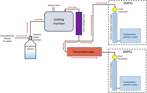
In our IVM setup (Figure 1), a TSI Constant Output Atomizer (model 3076, Shoreview, MN, USA) was used with 0.01% solution of the compound of interest dissolved in ultra-high purity water to aerosolize the compound. An air flow of approximately 3.3 L min⁻¹ filtered with a high-efficiency particulate air (HEPA) filter was used to produce the aerosol. The nebulizer output air flow (containing suspended liquid droplets) was then introduced into a mixing chamber (a large, stainless steel drum) to ensure that the aerosol is well-mixed. An air flow at a rate of 1.2 L min⁻¹ was pulled out of the mixing chamber and into a silica gel-containing diffusion drying tube, to bring the relative humidity of the air flow below the assumed efflorescence humidity of the aerosol (further elaboration is given in the Discussion section). The dried air flow was then split to flow through two separate scanning mobility particle sizers (SMPS), each sampling at a rate of 0.6 L min⁻¹. One (SMPS1 in Figure 1) measured the size distribution of room-temperature aerosol prior to entering a thermodenuder, while the other (SMPS2) measured the size distribution after the thermodenuder. The thermodenuder is a stainless steel tube with an inner diameter of 2.2 cm and 1 m in length (88 cm of which was heated), which, at 0.6 L min⁻¹ flow, resulted in a residence time of 33.5 s at room temperature and 21.1 s at 200 °C. Temperature data were recorded with a type-K thermocouple with a LabJack U6 (Lakewood, CO, USA) with data points recorded at 0.5-s intervals. Both SMPS systems are produced by TSI: the Condensation Particle Counter (CPC) 3789 and the Differential Mobility Analyzer (DMA) 3081 used with the Electrostatic Classifier 3082. Each electrostatic classifier was equipped with an x-ray aerosol neutralizer, the TSI Advanced Aerosol Neutralizer 3088. Classifiers were set to produce a single size distribution scan every 120 s. Both SMPS scan intervals were synchronized within 1 s of one another. For each compound, triplicate experiments were performed except for glucose, fructose, and leucine, which only had duplicate experiments due to instrumentation failures. From these distributions, the difference in total aerosol volume concentration between room temperature and a heated TD temperature were calculated. By slowly varying the temperature of the thermodenuder, data collected for aerosol volume concentration change Δv_p, heated temperature T₁, and reference temperature T₀ were used to fit for C_sat,0 and ΔH in Equation (1)(1) $$\Delta v_p=\frac{C_{\mathit{sat},0}}{{\rho }_p}\left[\exp \left(-\frac{\Delta H}{R}\left(\frac{1}{T_1}-\frac{1}{T_0}\right)\right)-1\right]\mathrm{ }$$(1) with knowledge of the density ρ_p of the compound. A characterization of particle losses in the thermodenuder with the nonvolatile sodium chloride aerosol within the experimental temperature range indicated losses of less than 5% above particle diameters of 80 nm (which contribute most significantly to the total aerosol volume). Differences in the counting between the two SMPS (up to 20%) were corrected for by comparing the total volume data of the two SMPS systems at room temperature before each experiment and then scaling the data at higher temperatures accordingly.

Figure 1. Integrated volume method experimental setup. Direction of air flow is indicated by red arrows.

According to Saleh, Shihadeh, and Khlystov (2011), for aerosol to reach equilibrium, the residence time in the thermodenuder should be more than 9 times greater than the aerosol characteristic time, which is a function of the aerosol size distribution and concentration. The ratios of the residence to characteristic times during our experiments are given in Table S2, all being above 10, thus satisfying the equilibration criteria.

2.2.2. The tandem differential mobility analyzer method for the volatility basis set determination of pollen extracts

To characterize the volatility of water-soluble pollen extracts (aspen and lodgepole pine), an approach approximating the overall evaporation behavior of a mixture of organic aerosol, known as the volatility basis set (Donahue et al. 2006; Donahue, Robinson, et al. 2012; Karnezi, Riipinen, and Pandis 2014; Stanier, Donahue, and Pandis 2008), is utilized. To create a VBS, saturation vapor concentration is expressed across a range of bins, spaced logarithmically (in our case from 10⁻⁵ μg m⁻³ to 10² µg m⁻³, a range that covers semi-volatile and low volatile compounds in the atmosphere).

In the TDMA setup, two DMAs, each equipped with aerosol neutralizers, are connected in tandem with a thermodenuder in between them, and a condensation particle counter (CPC) downstream (Tao and Mcmurry 1989). In this setup, one differential mobility analyzer selects a single electrical mobility diameter of aerosol from a sample and the single-size aerosol is flowed through a thermodenuder, where it will evaporate (decreasing in size) based on its residence time within the thermodenuder and the thermodenuder’s heated temperature. The second DMA and the CPC together act as an SMPS to record the size distribution of the resulting aerosol after evaporation. By varying the temperature in the thermodenuder, a relationship between aerosol diameter and temperature can be obtained.

To derive the VBS from tandem differential mobility analyzer (TDMA) measurements, we followed the common approach described elsewhere (Karnezi, Riipinen, and Pandis 2014; Saha et al. 2017). Briefly, the method consists in measuring temperature-dependent size changes of a quasi-monodisperse aerosol and iteratively solving a set of ordinary differential equations (ODE) to find the VBS that best matches the observations. The ODE set consists of mass loss rate equations of individual aerosol components: (2) $$\frac{d{m}_i}{dt}=-2\pi D{d}_{p}FK{{}^{\mathrm{*}}}_{\mathit{sat},i}{f}_i$$(2) with a constraint: (3) $$m_{\mathit{tot}}=\sum _i{m}_i\text{\hspace{1em}or\hspace{1em}}\sum _i{f}_i=1$$(3) where f_i is the mass fraction of the total organic mass with the effective saturation vapor pressure C*_sat, (compound’s individual saturation vapor concentration multiplied by its activity coefficient in the aerosol mixture). f_i represents the VBS and can also be written as m_i/m_tot, in which m_tot is the total organic mass (the sum of the mass of all C*_sat,i across the entire basis set) and m_i is the mass within an individual C*_sat,i bin. The particle diameter d_p is equal to (6 m_tot/πρ)^1/3. D is the diffusion coefficient of the compound in air, K is the Kelvin correction factor based on the curvature of the particle (assuming a spherical particle), and F is the Fuchs-Sutugin correction factor, dependent upon the accommodation coefficient α, or the ratio between the observed gas-liquid exchange rate of the particle to the maximum gas-liquid exchange rate of the particle based on kinetic theory of gases (Fuchs and Sutugin 1971; Maa 1967). For a more thorough discussion of the K and F correction equations, see Seinfeld and Pandis (2006).

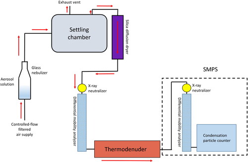
The experimental setup is shown in Figure 2. Liquid pollen extract solution (detailed in section 2.1) was aerosolized using a glass nebulizer from Amrita Aromatherapy Inc. (Fairfield, IA, USA) by a constant flow of HEPA-filtered air at approximately 3.3 L min⁻¹. This air flow (with liquid droplets in it, formed from the solution) flowed into a settling drum, from which the active flow pump in the CPC pulled 0.6 L min⁻¹ through a diffusion dryer to reduce the relative humidity (38.2 ± 0.5% for the lodgepole pine trials and 38.9 ± 0.2% for the aspen pollen trials). Then, the aerosol sample flowed into the leading DMA, thermodenuder, and SMPS that were the same as described in Section 2.2.1. The remaining 2.7 LPM flowed out of the settling drum to exhaust.

Figure 2. Flow setup of aerosol generation and TDMA setup. Red arrows indicate flow direction of air (aerosol sample).

Measurable quantities in the TDMA setup include the temperature of the thermodenuder and the resulting diameter that the aerosol attained after evaporation from its original monodisperse diameter selected by the leading DMA (examples given in Figure S1). By varying the thermodenuder temperature, C*_sat,i in Equation (2)(2) $$\frac{d{m}_i}{dt}=-2\pi D{d}_{p}FK{{}^{\mathrm{*}}}_{\mathit{sat},i}{f}_i$$(2) shifts via the Clausius-Clapeyron equation, and by observing the new diameter of the monodisperse aerosol at that C*_sat,i, we can determine the mass fraction that evaporates at each C*_sat,i.

For each sample, three trials each were performed for the monodisperse aerosol diameters of 100, 200, and 300 nm. The resulting evaporated mode diameter is recorded at each thermodenuder temperature, giving a set of temperature vs. diameter data. Data were manually inspected to ensure that the mode diameter always resided within the quasi-monodisperse distribution and not on a multiple-charged distribution. Data were then binned at intervals of 10 °K such that there were approximately 20 data points in each thermogram (spanning ∼298 °K to ∼398 °K).

To find the VBS, Equations (2)(2) $$\frac{d{m}_i}{dt}=-2\pi D{d}_{p}FK{{}^{\mathrm{*}}}_{\mathit{sat},i}{f}_i$$(2) and (3)(3) $$m_{\mathit{tot}}=\sum _i{m}_i\text{\hspace{1em}or\hspace{1em}}\sum _i{f}_i=1$$(3) were numerically solved for various VBS to generate modeled evaporation thermograms to find a VBS that produces the best fit to the experimental thermogram (experimental temperature vs. diameter data) via non-negative least squares fitting. In Equation (2)(2) $$\frac{d{m}_i}{dt}=-2\pi D{d}_{p}FK{{}^{\mathrm{*}}}_{\mathit{sat},i}{f}_i$$(2) , the diffusion coefficient, Fuchs-Sutugin factor, and Kelvin curvature effect were calculated using an assumed surface free energy and accommodation coefficient provided in Table S3, which we estimated from previous measurements on dicarboxylic acids (Saleh, Walker, and Khlystov 2008). Meanwhile, values of ΔH were approximated based on the results of ΔH from individual compounds via the IVM and relative abundance of these compounds measured in the extract (Axelrod, Samburova, and Khlystov 2021). Examples of modeled vs. experimental data are visualized in Figure S2. The modeled VBS producing the best-fit thermograms for each trial were averaged, and the average results along with the variability of individual runs are discussed in the Results and Discussion section (section 3.2).

3. Results and discussion

3.1. Saturation vapor concentration and latent heat of phase change of main chemical pollen constituents (IVM)

Figure 3 presents an example (proline) of data to which C_sat,0 and ΔH are fitted. The original raw data displays the difference Δv_p between heated aerosol volume concentration and reference aerosol volume concentration at a certain thermodenuder temperature in °C. Similar plots of all other compounds are given in Figure S3. For each compound, the particle had one distinctive volume loss curve. Minimum temperatures were selected based on observed change in volume and the measurement noise (most likely due to the counting uncertainty of either SMPS). Temperatures down to 30 °C were used for proline and GABA, as they exhibited stronger evaporation at lower temperatures than the other compounds tested. Temperatures above 50 °C were used for leucine, asparagine, fructose, and glucose, as these compounds showed less evaporation. Unlike the other compounds, most of the volume loss for sucrose occurred above 160 °C, and noise below this temperature resulted in low (∼0.94) R² values for the fitting. The minimum temperature used for sucrose was the minimum temperature with R² > 0.97, which was 138 °C. The R² values of the datasets of all other compounds were greater than 0.99. See Table S1 for full temperature ranges used for analysis of each compound.

Figure 3. Temperature vs. volume change data used for fitting of C_sat,0 and ΔH for proline and the modeled data generated by the fitted values of C_sat,0 and ΔH in Equation (3)(3) $$m_{\mathit{tot}}=\sum _i{m}_i\text{\hspace{1em}or\hspace{1em}}\sum _i{f}_i=1$$(3) . Data were binned and averaged at intervals of 2 °C (with standard deviations used for error bars) to prevent the Levenberg-Marquardt least-squares fitting algorithm from biasing the fit for lower temperatures, where a larger number of raw data points were taken. Plotted over the temperature-averaged data is also the modeled resultant curve generated from the fitted parameters of the IVM Equation (3)(3) $$m_{\mathit{tot}}=\sum _i{m}_i\text{\hspace{1em}or\hspace{1em}}\sum _i{f}_i=1$$(3) .

Table 1 above provides the fit results for amino acids and the saccharides utilizing the IVM. Figure S1 depicts the best-fit statistics of these parameters. In each case, a brute-force fitting method was utilized to confirm that the Levenberg-Marquardt least squares fitting method was finding the global minimum from a range of 35,000<ΔH < 500,000 J/mol and 0<C_sat,0<100 μg m⁻³. The errors given are the standard error of the modeled data produced by the fitted parameters. Additionally, measurements and estimations of these parameters from previous studies are given in Table 2.

Table 1. Fit results of C_sat,0 and ΔH for the tested bioaerosol compounds, calculated at 25 °C.

	Csat,0 at 25 °C (μg m^−3)	ΔH (kJ mol^−1)
L-Proline	17.5 ± 2.2	87.5 ± 3.3
L-Leucine	0.25 ± 0.06	104.2 ± 3.3
γ-aminobutyric acid (GABA)	14.7 ± 0.8	68.9 ± 1.1
L-Asparagine	0.049 ± 0.006	79.3 ± 1.2
D-Glucose	0.034 ± 0.006	106.8 ± 2.2
Sucrose	0.0010 ± 0.0006	86.2 ± 4.4
D-Fructose	4.4 ± 0.5	70.1 ± 2.1

Note: See Table S1 for full experimental statistics on temperatures and relative humidities.

Table 2. Summary of previous studies measuring or modeling ΔH for the seven compounds of interest in this study.

	ΔH (kJ/mol)	Method	Reference
Leucine	148.7 ± 6.5	Thermogravimetric	Lähde et al. (2009)
	151.0 ± 0.8	Knudsen effusion	Svec and Clyde (1965)
	139.8	Modeled G4 theory calculations	Dorofeeva and Ryzhova (2014)
Proline	96.7 ± 0.8	Knudsen effusion	Svec and Clyde (1965)
	127.3 ± 1.0	Knudsen effusion	Santos et al. (2014)
	127.4 ± 1.0	Torsion and weighing effusion	De Kruif et al. (1979)
	125.7 ± 4.0	Modeled G4 theory calculations	Dorofeeva and Ryzhova (2014)
Asparagine	174.2 ± 4.0	Modeled G4 theory calculations	Dorofeeva and Ryzhova (2014)
	188.04	Joback group contribution method	Chemeo database
GABA	139 ± 4	Thermogravimetric	Legendre et al. (2009)
	140 ± 2	Calorimetry	Sabbah and Skoulika (1983)
	139.1 ± 3.0	Modeled G4 theory calculations	Dorofeeva and Ryzhova (2014)
Fructose	143.67	Joback group contribution method	Chemeo database
Glucose	194.4 ± 5.0	Knudsen effusion	Oja and Suuberg (1999)
	132.44	Joback group contribution method	Chemeo database
Sucrose	248.19	Joback group contribution method	Chemeo database

Among all the compounds tested, proline had the highest saturation vapor concentration (17.5 ± 2.2 μg m⁻³), indicating that it has the most volatile behavior in aerosol form. Other compounds that were in the semi-volatile range included GABA (14.7 ± 0.8 μg m⁻³) and fructose (4.4 ± 0.5 μg m⁻³). Low-volatile compounds tested included leucine (0.25 ± 0.06 μg m⁻³), glucose (0.034 ± 0.006 μg m⁻³), asparagine (0.049 ± 0.006 μg m⁻³), and sucrose (0.0010 ± 0.0006 μg m⁻³), though sucrose was within one order of magnitude to the level of extremely-low volatile classification (Donahue, Kroll, et al. 2012). From these results, it can be determined that if each compound existed in the atmosphere at the same concentration, proline and GABA are the most likely to exist in the gas phase in the atmosphere and sucrose the least likely, though the actual mass fraction that would exist in the gas phase also depends heavily on total organic aerosol mass concentration in the air (Donahue et al. 2006).

When compared to the measured saturation vapor concentrations of other compounds in previous research, proline, GABA, and fructose fall within the volatility ranges of sugar alcohols (meso-erythritol: 3.1 to 103.5 μg m⁻³ depending on kinetic assumptions) (Emanuelsson, Tschiskale, and Bilde 2016) and straight-chain dicarboxylic acids (often between 0.1 and 100 μg m⁻³ in the solid state) (Bilde et al. 2015).

The latent heats of phase change of the seven compounds tested ranged from 68.9 ± 1.1 to 106.8 ± 2.1 kJ mol⁻¹ (GABA and glucose, respectively). When compared to previous literature on measurements and estimations of the latent heat of these compounds, our results were lower. For example, the lowest estimate made for the latent heat of sublimation of proline is 96.7 kJ mol⁻¹ by Svec and Clyde (1965), of which our measurement is nearly 10 kJ mol⁻¹ lower (Table 2). GABA had the most consistent estimates of its latent heat of sublimation in previous studies, between 139 and 140 kJ mol⁻¹ (Dorofeeva and Ryzhova 2014; Legendre et al. 2009; Sabbah and Skoulika 1983), but our result was considerably lower, at 68.9 ± 1.1 kJ mol⁻¹. From this, we hypothesize that we measured the latent heat of vaporization (from subcooled liquid to gas), and not the latent heat of sublimation (from crystalline solid to gas) (Bilde et al. 2015).

Furthermore, Figure S4 shows Arrhenius graphs depicting the modeled saturation vapor pressure behavior (converted from saturation vapor concentration) of three compounds in our study compared to the behavior of these compounds in previous studies using Knudsen effusion methods to measure vapor pressures at elevated temperatures. In all cases, the relation between vapor pressure and temperature indicates that our study displayed higher vapor pressures at room temperature than previous studies. This is further an indication that the condensed phase in our experiments was the subcooled liquid state.

In the setup utilizing the silica gel diffusion dryer, relative humidity (RH) of the aerosol flow was difficult to hold constant, as the silicate would need to be replaced frequently in order to hold the relative humidity to below 40% (measured with the RH sensor built into the TSI 3082 Electrostatic Classifier, which controls the DMA) (see Table S1 for full RH ranges of all compounds). The efflorescence RH of multiple amino acids has been measured to be 40% or above, and often vary among the exact RH reported between studies (Chan et al. 2005; Guo et al. 2020; Yang et al. 2020). Efflorescence behavior of the three specific amino acids that we tested is not available to our knowledge, though hygroscopicity of crystalline bulk material has been measured; for example, proline becomes anhydrous at RH ∼31% (Mellon and Hoover 1951)). Previous research also showed that sucrose and glucose aerosol, meanwhile, do not have distinct observed efflorescence points but display growth factors of less than 1.1 under 40% RH (Estillore et al. 2017). Fructose shows similar behavior (Chan, Kreidenweis, and Chan 2008). Due to the fact that these compounds are not shown to undergo distinct efflorescence, and because of the unknown efflorescence points of the amino acids, it cannot be confirmed that the aerosol generated in our experiments did not contain small amounts of water, existing in a state of subcooled liquid. Due to the unknown efflorescence points of many compounds, it is generally preferred that RH should be as low as possible, ideally less than 10%, when performing the IVM (Bilde et al. 2015). Meanwhile, one of our experiments had RH as high as 45% (GABA, see Table S1 for full summary of experimental RH). Because efflorescence was not monitored in this study, generated aerosols could have existed as subcooled liquid droplets. It should be noted that the subcooled state is likely to be more atmospherically relevant than the dry, crystallized state (Bilde et al. 2015), as biological compounds found in pollen are more likely to be released from pollen via osmotic rupture in high-humidity conditions as previously discussed (Hughes et al. 2020; Miguel et al. 2006; Steiner et al. 2015).

An important discussion regarding the usage of atmospherically-nonrelevant temperatures to extrapolate the thermodynamic properties of a compound at room temperature is whether the elevated temperatures result in thermal decomposition/pyrolysis of the compound rather than evaporation/sublimation. In this supposed case, the compound of interest thermally decomposes into other compounds (e.g., fructose and glucose decomposing to a variety of furan derivatives, pyran derivatives, and aldehydes among many others (Moldoveanu 2019). However, in many other previous studies, the thermal decomposition of the compounds tested occur at temperatures higher than the temperatures at which we observed aerosol volume loss. Glucose pyrolysis temperature starts between 153 and 156 °C, (Moldoveanu 2019), while experiments intended to produce vacuum pyrolysis products of glucose and fructose were conducted at 275 °C (Ponder and Richards 1993). Fast pyrolysis product analysis has been performed on fructose, requiring temperatures from 250 to 500 °C (Zhang et al. 2013). Glucose is observed to pyrolyze in acidic conditions at lower temperatures, as low as 60 °C (Long et al. 2018). But the conditions of our experiments were not acidic, and glucose has been observed (in aqueous form) to be thermally stable at 150 °C in acid-free conditions (Pilath et al. 2010).

Thermogravimetric experiments of leucine in bulk showed that leucine sublimates at approximately 295 °C, remaining chemically stable until ∼303 °C (Li et al. 2006). Several amino acids were observed to decompose in saturated subcritical water conditions between 230 to 253 °C, sometimes decomposing into other amino acids (Abdelmoez, Yoshida, and Nakahasi 2010). Proline decomposes thermally between 220 and 290 °C (Schaberg, Wroblowski, and Goertz 2018) and asparagine began to decompose at a similar temperature or higher (Schaberg, Wroblowski, and Goertz 2018; Weiss et al. 2018). However, all of these experiments were performed at temperatures that we do not reach in the thermodenuder. In biological mixtures, GABA was shown to decrease after heating between 80 and 120 °C after 30 min (Jirasatid and Nopharatana 2021). However, our volume-loss-temperature observed was lower than these temperatures, for significantly less exposure time, and in pure form rather than in mixtures.

Disaccharides like sucrose begin to decompose around 190 °C (Moldoveanu 2019), which is in the range of temperature at which we observed volume loss. Therefore, it can be assumed that sucrose was the only compound we tested in which thermal decomposition in the thermodenuder may have occurred. However, sucrose also was our least-volatile compound tested in terms of its saturation vapor pressure, and thus is surmised to be fully condensed in the atmosphere.

3.2. Characterization of volatility of water-soluble pollen extracts (VBS)

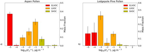
The volatility basis sets of aspen and lodgepole pine pollen extracts were calculated and are given in Figures 4a and b. To solve Equations (2)(2) $$\frac{d{m}_i}{dt}=-2\pi D{d}_{p}FK{{}^{\mathrm{*}}}_{\mathit{sat},i}{f}_i$$(2) and (3)(3) $$m_{\mathit{tot}}=\sum _i{m}_i\text{\hspace{1em}or\hspace{1em}}\sum _i{f}_i=1$$(3) for the mass fraction of compounds within a specific order of magnitude of effective saturation vapor pressure, a total of nine trials were performed in the TDMA setup for each pollen extract. These nine trials included three trials each of which an aerosol size of 100, 200, and 300 nm were selected by the leading DMA. For each trial, a separate VBS mass fraction distribution was calculated at a 25 °C reference temperature, and these nine distributions were averaged to produce the results presented in Figure 4. The relative humidity was 38.2 ± 0.5% for the lodgepole pine pollen trials and 38.9 ± 0.2% for the aspen pollen trials.

Figure 4. Volatility basis sets for (a) aspen pollen and (b) lodgepole pine pollen.

Assumed parameters included the Kelvin curvature effect, which was calculated with a surface free energy of 0.18 J m⁻², the average of the measured surface free energies of adipic, succinic, and pimelic acid (Saleh, Shihadeh, and Khlystov 2009). Though these are dicarboxylic acids, a different compound group from the ones we tested with the IVM, they were nonetheless selected as they are some of the few compounds in which surface free energy in aerosol form is known. Another assumed parameter was the accommodation coefficient α, which has been shown to affect the calculation of saturation vapor concentration by orders of magnitude (Emanuelsson, Tschiskale, and Bilde 2016). Like surface free energy, the accommodation coefficient is not well studied for individual compounds, and as such we selected a value of 0.13, the average accommodation coefficient of three dicarboxylic acids (Saleh, Shihadeh, and Khlystov 2009)

Parameters also approximated included the density, molecular weight, and latent heat of phase change estimated from the IVM results on individual compounds and their relative abundances to one another in pollen (Axelrod, Samburova, and Khlystov 2021). Mean free path and diffusion coefficient in air were estimated via their relative abundances and group contribution methods from (Poling, Prausnitz, and O’Connell 2001). A summary of the parameters used for each pollen extract is given in Table S3.

There was significant uncertainty calculated in individual volatility bins, specifically the log(C*_sat,i)= [−4] bin for aspen pollen, and the log₁₀(C*_sat,i)= [−4, −2, 0] bins for lodgepole pine pollen. This uncertainty can be explained by slight differences in the thermograms in each trial resulting in mass fraction being predicted larger in a bin next to (either lower or higher) than the average bin. The SVOC, LVOC, and ELVOC were totaled for each trial and their averages and standard deviations calculated, and the fractional uncertainty was significantly reduced in comparison to the logarithmically spaced size bin data. The percentages quoted below are the totals for each of these three volatility categorizations.

For aspen pollen extract, approximately 37.8 ± 2.4% of mass is extremely-low volatile, 53.7 ± 3.0% is low volatile, and 8.5 ± 3.5% is semivolatile. For lodgepole pine pollen extract, approximately 35.4 ± 5.6% of mass is extremely-low volatile, 62.4 ± 6.9% is low volatile, and 2.2 ± 2.7% is semivolatile (i.e., the amount of semivolatile material in lodgepole pine pollen is highly uncertain). Individual VBS bins vary considerably between the two pollen species: in the LVOC range, 9.5 ± 3.3% (aspen) and 42.1 ± 6.0% (lodgepole pine) of masses have saturation vapor pressures on the order of 10⁻³ μg m⁻³, while in the ELVOC range 37.1 ± 2.5% of aspen pollen mass and 17.0 ± 10.2% of lodgepole pine pollen mass are on the order of 10⁻⁵ μg m⁻³ or lower. Meanwhile, in the SVOC range, aspen pollen has higher mass fractions than lodgepole pine in 10⁰ μg m⁻³ bin (7.7 ± 3.1% and 1.7 ± 2.4%, respectively), while mass fractions in the 10¹ and 10² μg m⁻³ bins combined are only ∼11% of the mass fraction in the 10⁰ μg m⁻³ bin for aspen and 30% for lodgepole pine pollen. This indicates that aspen pollen in the atmosphere may contribute nearly four times the semivolatile amount per unit pollen mass than lodgepole pine pollen. Meanwhile, lodgepole pine pollen has compounds with higher effective saturation vapor concentrations among those within the ELVOC range. These results indicate that different pollen species may have different volatility profiles. As such, other pollen species, especially those that contribute a major fraction of total emitted pollen in the atmosphere, as well as other major bioaerosols (Després et al. 2012), should be studied for their volatility profile.

Previous studies have quantified mass fractions of ambient aerosols in various locations. Mass fractions of ambient aerosol in the semivolatile range are generally between 0.4 and 0.7, variable across several cities such as urban areas in North Carolina, US (Saha et al. 2017), Mexico City (Cappa and Jimenez 2010), Paris (Paciga et al. 2016), Beijing (Xu et al. 2019) and Seoul (Kang et al. 2022), all of which constitute mass factions above those found for pollen extracts in this study. Mass fractions of semivolatiles from smog-chamber experiments for SOA formed from oxidation of BVOCs like α-pinene are significantly higher (0.85–0.92) (Saha and Grieshop 2016) than the semivolatile fraction of our pollen samples.

4.3. Estimation of bioaerosol contributions to ambient SVOC and LVOC

It is difficult to precisely estimate the contribution of aspen and lodgepole pine pollen to the total semivolatile organic carbon budget in the atmosphere due to a number of quantities that are either unknown or highly variable. Here we will attempt an upper-bound, order of magnitude estimation of how much pollen could contribute to the different volatility fractions of ambient aerosol. If we take the total global emission budget of pollen in the atmosphere to be 65 Tg yr⁻¹, the middle of the range of values in Després et al. (2012), and assume it was all exposed to high humidity conditions and ruptured into SPP at a rate of 70%, as shown by Chinese elm pollen under 98% relative humidity and in water droplets (Miguel et al. 2006), then the mass of 45.5 Tg yr⁻¹ of ruptured pollen could be exposed in the atmosphere. To our knowledge, the percent of the total pollen mass that is water soluble is not well characterized, but for the purpose of this discussion we will assume it to be 100%. Furthermore, the global fluxes of specific species of pollen, like aspen and lodgepole pine pollen, are not available to our knowledge. If we assume all of the 45.5 Tg yr⁻¹ flux to have the VBS similar to that of lodgepole pine, then a total of 1.0 Tg yr⁻¹ would be in the SVOC range and 28.4 Tg yr⁻¹ in the LVOC range. Meanwhile, if the total flux had a VBS profile similar to that of aspen pollen, a total of 3.9 Tg yr⁻¹ would be in the SVOC range and 24.1 Tg yr⁻¹ in the LVOC range. In comparison, with global fluxes of primary organic aerosol (POA) from biomass burning being ∼54 Tg yr⁻¹ (Andreae and Rosenfeld 2008), which have been estimated to contain ∼40% LVOCs and ∼50% SVOCs (Louvaris et al. 2017) (though highly variable based on location and fuel type) (Huffman et al. 2009), LVOC flux of this aerosol would be ∼21.6 Tg yr⁻¹ and SVOC flux would be 27 Tg yr⁻¹. As such, LVOC fluxes due to pollen could be comparable to that of biomass burning, and SVOC fluxes would be less than biomass burning but nonetheless non-negligible, at 4–14% of the flux of biomass burning. While our estimates of the pollen contribution to the total global fluxes in ELVOC, LVOC and SVOC classes is highly uncertain and likely represents an upper-end estimate, it demonstrates that pollen could provide a significant contribution to these volatility classes and further research is needed to better constrain the contribution of pollen to ambient aerosol VBS emission fluxes.

Comprehensive estimates for the near-surface air mass concentration of pollen on a species-by-species basis are not well studied. However, following Manninen et al. (2014) for studies of boreal forests, concentrations of pollen in near-surface air average 5.9 μg m⁻³ during pollen season, and may reach a maximum of 26 to 98 μg m⁻³. Though the distribution of pollinating species is diverse and varies ecosystem-by-ecosystem, if we were to assume that a hypothetical forest dominated by lodgepole pine in terms of pollen emission (liberally assuming pollen emissions by mass is 100% lodgepole pine pollen) were to have a similar average pollen concentration in near-surface air during pollen season, with 70% (by mass) of pollen grains rupturing to form SPP and 2.2% of such mass in the SVOC range, then an approximate concentration of SVOCs in the air would be 0.1 μg m⁻³. In the LVOC range (62.4% of total mass via the VBS), the concentration in air would be 2.6 μg m⁻³. However, a similar forest dominated by aspen as the primary pollinator (liberally assuming 100% of pollen mass is aspen pollen) would result in an average near-surface SVOC concentration of ∼0.3 μg m⁻³ and LVOC concentration of 2.2 μg m⁻³. Furthermore, using the maximum pollen concentration of 98 μg m⁻³ measured by Manninen et al. (2014), the SVOC concentration from aspen pollen in the air would be 5.8 μg m⁻³ and the LVOC concentration would be 36.8 μg m⁻³. Comparatively, if the urban air mass fraction of SVOCs was 0.6 and LVOCs was 0.25 following Saha et al. (2017) and the total organic mass in the air was 5 μg m⁻³, then SVOCs would constitute 3 μg m⁻³ and LVOCs would constitute 1.25 μg m⁻³. This general analysis, while very approximate, is an indication that during pollen season, pollen may contribute significantly to the SVOC and LVOC concentration in city-rural interface areas where both anthropogenic urban emissions and forest emissions are present. Furthermore, while the actual chemical changes that occur to pollen constituents in the atmosphere is not well-characterized and difficult to speculate, it should be noted that their presence in the air contributes to the total organic aerosol mass concentration, and thus influences aerosol-gas partitioning of other SVOCs in the atmosphere from other sources as well (Donahue et al. 2006).

These scenarios contain liberal estimates for percentages of each pollen species as a fraction of total aerosolized pollen mass (100%), percent of pollen that produces SPP (70%), and percent of water-soluble mass of pollen to total mass (100%). Furthermore, they also assume that semivolatile constituents of pollen can only be exposed to the atmosphere via osmotic rupture into SPP and not via other processes. Nonetheless, they should be considered as contributors to the total ambient LVOC and SVOC concentration in air, especially in forest settings.

A potential major source of uncertainty in our analysis stems from the estimate used for the accommodation coefficient, which has been known to cause uncertainty in the modeling of aerosol kinetics (Bilde et al. 2015; Cappa and Jimenez 2010). Due to this, we performed the VBS analysis for accommodation coefficients of 0.1 and 1.0, for each pollen sample, included in Figure S5. The general effect of increasing the accommodation coefficient by one order of magnitude (from 0.1 to 1.0) is to shift the overall VBS distribution by one order of magnitude of C*_sat lower. As a result, this causes great uncertainty in total SVOC mass fraction for aspen pollen and total LVOC mass fraction for lodgepole pine pollen. With α = 0.1, the total SVOC mass fraction in aspen pollen is 11.6%, versus 0.9% with α = 1.0, as a result of a significant mass fraction shifting between the low end of the SVOC range to the high end of the LVOC range. A similar type of shift is noted between the LVOC and ELVOC ranges for lodgepole pine pollen. In either scenario, however, the VBS distributions for these pollens have an overall lower volatility than the urban ambient VBS of Cappa and Jimenez (2010).

From our results, it can be determined that the majority of the water-soluble masses of both aspen and lodgepole pine pollen are low volatile or extremely-low volatile. However, with pollen seasons expected to increase in release and duration with rising temperatures (Anderegg et al. 2021) and aspen tree populations rising with carbon dioxide levels (Cole et al. 2009) in the atmosphere, it is important to note that up to 8.5% of water-soluble aspen pollen mass is semivolatile, more than four times higher than the SVOC percentage of water-soluble lodgepole pine pollen mass. This establishes a difference between two different pollen species in terms of volatility, demonstrating the need for future research on the semivolatile composition of other major species of atmospherically relevant pollen and their relative contributions of SVOC to other sources in the atmosphere. It should be noted that if the main contributors of the semivolatile mass fraction of aspen pollen are semivolatile amino acids and saccharides, the possibility exists that other biological particles other than pollen (which contain these compounds) can contribute to the total SVOC budget in the atmosphere via these compounds as well. Further research is needed to more accurately determine the percent of atmospheric exposure of SVOC constituents of pollen so that aerosol-gas partitioning of these compounds can be more accurately estimated in an ambient setting.

4. Conclusions

In this research, the integrated volume method was used to characterize volatility behavior (via quantifying the saturation vapor concentrations and latent heats of phase change) for seven compounds (four amino acids and three saccharides) found in water-soluble pollen extract. Of these, proline, γ-aminobutyric acid (GABA), and fructose had saturation vapor concentrations in the semivolatile range from 3 × 10⁻¹ to 3 x 10² μg m⁻³. In our experiments, the possibility exists that we measured the saturation vapor concentrations and latent heats of subcooled liquid droplets of these compounds, but the information nonetheless remains atmospherically relevant as this is their most likely state in aerosol form in the atmosphere. Furthermore, the volatility basis set approach was used to characterize the volatility of the water soluble extracts of two different species of pollen: aspen and lodgepole pine. There were noticeable differences in the VBS between the two species, with aspen having up to 8.5% of its mass being semivolatile. This shows that pollen could provide a substantial contribution to the total SVOC concentration in air during pollen season. However, future research is required in order to estimate the precise total fluxes of these compounds in the atmosphere and their concentrations in ambient air so that their relative contribution of SVOCs to the atmosphere can be compared to other sources. In turn, this may determine if pollen could have an appreciable effect on atmospheric chemical processes.

Acknowledgments

The authors would like to thank Dr. Alison Murray of the Desert Research Institute for assistance in sample preparation.

Disclosure statement

No potential conflicts of interest was reported by the author(s).

Additional information

Funding

This work is supported by the National Science Foundation under Grant No. AGS-1760328.

References

- Abdelmoez, W., H. Yoshida, and T. Nakahasi. 2010. Pathways of amino acid transformation and decomposition in saturated subcritical water conditions. Int. J. Chem. React. Eng. 8 (1):5286–94. doi: 10.2202/1542-6580.1903.
- Anderegg, W. R. L., J. T. Abatzoglou, L. D. L. Anderegg, L. Bielory, P. L. Kinney, and L. Ziska. 2021. Anthropogenic climate change is worsening North American pollen seasons. Proc. Natl. Acad. Sci. U S A 118 (7):1–6. doi: 10.1073/pnas.2013284118.
- Andreae, M. O., and D. Rosenfeld. 2008. Aerosol-cloud-precipitation interactions. Part 1. The nature and sources of cloud-active aerosols. Earth-Sci. Rev. 89 (1-2):13–41. doi: 10.1016/j.earscirev.2008.03.001.
- Axelrod, K., V. Samburova, and A. Y. Khlystov. 2021. Relative abundance of saccharides, free amino acids, and other compounds in specific pollen species for source profiling of atmospheric aerosol. Sci. Total Environ. 799:149254. doi: 10.1016/j.scitotenv.2021.149254.
- Barley, M. H., and G. McFiggans. 2010. The critical assessment of vapour pressure estimation methods for use in modelling the formation of atmospheric organic aerosol. Atmos. Chem. Phys. 10 (2):749–67. doi: 10.5194/acp-10-749-2010.
- Bedinger, P. 1992. The remarkable biology of pollen. Plant Cell. 4 (8):879–87. doi: 10.1105/tpc.4.8.879.
- Bilde, M., K. Barsanti, M. Booth, C. D. Cappa, N. M. Donahue, E. U. Emanuelsson, G. McFiggans, U. K. Krieger, C. Marcolli, D. Topping, et al. 2015. Saturation vapor pressures and transition enthalpies of low-volatility organic molecules of atmospheric relevance: from dicarboxylic acids to complex mixtures. Chem. Rev. 115 (10):4115–56. doi: 10.1021/cr5005502.
- Bilde, M., B. Svenningsson, J. Mønster, and T. Rosenørn. 2003. Even-odd alternation of evaporation rates and vapor pressures of C3-C9 dicarboxylic acid aerosols. Environ. Sci. Technol. 37 (7):1371–8. doi: 10.1021/es0201810.
- Cao, L. M., X. F. Huang, Y. Y. Li, M. Hu, and L. Y. He. 2018. Volatility measurement of atmospheric submicron aerosols in an urban atmosphere in southern China. Atmos. Chem. Phys. 18 (3):1729–43. doi: 10.5194/acp-18-1729-2018.
- Cappa, C. D., and J. L. Jimenez. 2010. Quantitative estimates of the volatility of ambient organic aerosol. Atmos. Chem. Phys. 10 (12):5409–24. doi: 10.5194/acp-10-5409-2010.
- Card, M. L., V. Gomez-Alvarez, W. H. Lee, D. G. Lynch, N. S. Orentas, M. T. Lee, E. M. Wong, and R. S. Boethling. 2017. History of EPI SuiteTM and future perspectives on chemical property estimation in US Toxic Substances Control Act new chemical risk assessments. Environ. Sci. Process. Impacts. 19 (3):203–12. doi: 10.1039/c7em00064b.
- Chan, M. N., M. Y. Choi, N. L. Ng, and C. K. Chan. 2005. Hygroscopicity of water-soluble organic compounds in atmospheric aerosols: Amino acids and biomass burning derived organic species. Environ. Sci. Technol. 39 (6):1555–62. doi: 10.1021/es049584l.
- Chan, M. N., S. M. Kreidenweis, and C. K. Chan. 2008. Measurements of the hygroscopic and deliquescence properties of organic compounds of different solubilities in water and their relationship with cloud condensation nuclei activities. Environ. Sci. Technol. 42 (10):3602–8. doi: 10.1021/es7023252.
- Cole, C. T., J. E. Anderson, R. L. Lindroth, and D. M. Waller. 2009. Rising concentrations of atmospheric CO2 have increased growth in natural stands of quaking aspen (Populus tremuloides). Glob. Chang. Biol. 16 (8):2186–97. doi: 10.1111/j.1365-2486.2009.02103.x.
- D’Amato, G., H. J. Chong-Neto, O. P. Monge Ortega, C. Vitale, I. Ansotegui, N. Rosario, T. Haahtela, C. Galan, R. Pawankar, M. Murrieta-Aguttes, et al. 2020. The effects of climate change on respiratory allergy and asthma induced by pollen and mold allergens. Allergy Eur. J. Allergy Clin. Immunol. 75 (9):2219–28. doi: 10.1111/all.14476.
- De Kruif, C. G., J. Voogd, and J. Offringa. 1979. Enthalpies of sublimation and vapour pressures of 14 amino acids and peptides. J.Chem. Thermodyn. 11 (7):651–6. doi: 10.1016/0021-9614(79)90030-2.
- Després, V. R., J. Alex Huffman, S. M. Burrows, C. Hoose, A. S. Safatov, G. Buryak, J. Fröhlich-Nowoisky, W. Elbert, M. O. Andreae, U. Pöschl, et al. 2012. Primary biological aerosol particles in the atmosphere: A review. Tellus, Ser. B Chem. Phys. Meteorol. 64 (1):15598. doi: 10.3402/tellusb.v64i0.15598.
- Donahue, N. M., J. H. Kroll, S. N. Pandis, and A. L. Robinson. 2012. A two-dimensional volatility basis set-Part 2: Diagnostics of organic-aerosol evolution. Atmos. Chem. Phys. 12 (2):615–34. doi: 10.5194/acp-12-615-2012.
- Donahue, N. M., A. L. Robinson, C. O. Stanier, and S. N. Pandis. 2006. Coupled partitioning, dilution, and chemical aging of semivolatile organics. Environ. Sci. Technol. 40 (8):2635–43. doi: 10.1021/es052297c.
- Donahue, N. M., A. L. Robinson, E. R. Trump, I. Riipinen, and J. H. Kroll. 2012. Volatility and aging of atmospheric organic aerosol. Top Curr. Chem. 339:1–26. doi: 10.1007/128.
- Dorofeeva, O. V., and O. N. Ryzhova. 2014. Gas-phase enthalpies of formation and enthalpies of sublimation of amino acids based on isodesmic reaction calculations. J. Phys. Chem. A 118 (19):3490–502. doi: 10.1021/jp501357y.
- Emanuelsson, E. U., M. Tschiskale, and M. Bilde. 2016. Phase state and saturation vapor pressure of submicron particles of meso-erythritol at ambient conditions. J. Phys. Chem. A 120 (36):7183–91. doi: 10.1021/acs.jpca.6b04349.
- Estillore, A. D., H. S. Morris, V. W. Or, H. D. Lee, M. R. Alves, M. A. Marciano, O. Laskina, Z. Qin, A. V. Tivanski, and V. H. Grassian. 2017. Linking hygroscopicity and the surface microstructure of model inorganic salts, simple and complex carbohydrates, and authentic sea spray aerosol particles. Phys. Chem. Chem. Phys. 19 (31):21101–11. doi: 10.1039/c7cp04051b.
- Estillore, A. D., J. V. Trueblood, and V. H. Grassian. 2016. Atmospheric chemistry of bioaerosols: Heterogeneous and multiphase reactions with atmospheric oxidants and other trace gases. Chem. Sci. 7 (11):6604–16. doi: 10.1039/c6sc02353c.
- Fröhlich-Nowoisky, J., C. J. Kampf, B. Weber, J. A. Huffman, C. Pöhlker, M. O. Andreae, N. Lang-Yona, S. M. Burrows, S. S. Gunthe, W. Elbert, et al. 2016. Bioaerosols in the Earth system: Climate, health, and ecosystem interactions. Atmos. Res. 182:346–76. doi: 10.1016/j.atmosres.2016.07.018.
- Fuchs, N. A., and A. G. Sutugin. 1971. High-Dispersed Aerosols. In Topics in Current Aerosol Research, eds. G. M. Hidy and J. R. Brock. Oxford: Pergamon Press.
- Guo, Y., N. Wang, S. Pang, and Y. Zhang. 2020. Hygroscopic properties and compositional evolution of internally mixed sodium nitrate-amino acid aerosols. Atmos. Environ. 242 (December 2019):117848. doi: 10.1016/j.atmosenv.2020.117848.
- Huffman, J. A., K. S. Docherty, C. Mohr, M. J. Cubison, I. M. Ulbrich, P. J. Ziemann, T. B. Onasch, and J. L. Jimenez. 2009. Chemically-resolved volatility measurements of organic aerosol from different sources. Environ. Sci. Technol. 43 (14):5351–7. doi: 10.1021/es803539d.
- Hughes, D. D., C. B. A. Mampage, L. M. Jones, Z. Liu, and E. A. Stone. 2020. Characterization of atmospheric pollen fragments during springtime thunderstorms. Environ. Sci. Technol. Lett. 7 (6):409–14. doi: 10.1021/acs.estlett.0c00213.
- Jirasatid, S., and M. Nopharatana. 2021. Thermal kinetics of gamma–aminobutyric acid and antioxidant activity in germinated red jasmine rice milk using Arrhenius, Eyring-Polanyi and ball models. Curr. Res. Nutr. Food Sci. 9 (2):700–11. doi: 10.12944/CRNFSJ.9.2.33.
- Kang, H. G., Y. Kim, S. Collier, Q. Zhang, and H. Kim. 2022. Volatility of Springtime ambient organic aerosol derived with thermodenuder aerosol mass spectrometry in Seoul, Korea. Environ. Pollut. 304 (March):119203. doi: 10.1016/j.envpol.2022.119203.
- Karnezi, E., I. Riipinen, and S. N. Pandis. 2014. Measuring the atmospheric organic aerosol volatility distribution: A theoretical analysis. Atmos. Meas. Tech. 7 (9):2953–65. doi: 10.5194/amt-7-2953-2014.
- Kavouras, I. G., N. Mihalopoulos, and E. G. Stephanou. 1998. Formation of atmospheric particles from organic acids produced by forests. Nature 395 (6703):683–6. doi: 10.1038/27179.
- Kim, K. H., E. Kabir, and S. A. Jahan. 2018. Airborne bioaerosols and their impact on human health. J. Environ. Sci. 67:23–35. doi: 10.1016/j.jes.2017.08.027.
- Komkoua Mbienda, A. J., C. Tchawoua, D. A. Vondou, and F. Mkankam Kamga. 2013. Evaluation of vapor pressure estimation methods for use in simulating the dynamic of atmospheric organic aerosols. Int. J. Geophys. 2013 (2):1–13. doi: 10.1155/2013/612375.
- Lähde, A., J. Raula, J. Malm, E. I. Kauppinen, and M. Karppinen. 2009. Sublimation and vapour pressure estimation of l-leucine using thermogravimetric analysis. Thermochim. Acta. 482 (1–2):17–20. doi: 10.1016/j.tca.2008.10.009.
- Laothawornkitkul, J., J. E. Taylor, N. D. Paul, and C. N. Hewitt. 2009. Biogenic volatile organic compounds in the Earth system: Tansley review. New Phytol. 183 (1):27–51. doi: 10.1111/j.1469-8137.2009.02859.x.
- Legendre, B., P. Bac, M. German, and Y. Feutelais. 2009. Low pressure phases: Thermodynamic properties of the γ-aminobutyric acid. J. Therm. Anal. Calorim. 98 (1):91–5. doi: 10.1007/s10973-009-0401-0.
- Li, J., Z. Wang, X. Yang, L. Hu, Y. Liu, and C. Wang. 2006. Decomposing or subliming? An investigation of thermal behavior of l-leucine. Thermochim. Acta 447 (2):147–53. doi: 10.1016/j.tca.2006.05.004.
- Li, K., J. Liggio, P. Lee, C. Han, Q. Liu, and S.-M. Li. 2019. Secondary organic aerosol formation from α-pinene, alkanes, and oil-sands-related precursors in a new oxidation flow reactor. Atmos. Chem. Phys. 19 (15):9715–31. doi: 10.5194/acp-19-9715-2019.
- Long, Y., Y. Yu, B. Song, and H. Wu. 2018. Polymerization of glucose during acid-catalyzed pyrolysis at low temperatures. Fuel 230 (March):83–8. doi: 10.1016/j.fuel.2018.05.022.
- Louvaris, E. E., K. Florou, E. Karnezi, D. K. Papanastasiou, G. I. Gkatzelis, and S. N. Pandis. 2017. Volatility of source apportioned wintertime organic aerosol in the city of Athens. Atmos. Environ 158:138–47. doi: 10.1016/j.atmosenv.2017.03.042.
- Maa, J. R. 1967. Evaporation coefficient of liquids. Ind. Eng. Chem. Fund. 6 (4):504–18. doi: 10.1021/i160024a005.
- Manninen, H. E., S. L. Sihto-Nissilä, V. Hiltunen, P. P. Aalto, M. Kulmala, T. Petäjä, H. E. Manninen, J. Bäck, P. Hari, J. A. Huffman, et al. 2014. Patterns in airborne pollen and other primary biological aerosol particles (PBAP), and their contribution to aerosol mass and number in a boreal forest. Boreal Environ. Res. 19 (September):383–405.
- McGenity, T. J., A. T. Crombie, and J. C. Murrell. 2018. Microbial cycling of isoprene, the most abundantly produced biological volatile organic compound on Earth. ISME J. 12 (4):931–41. doi: 10.1038/s41396-018-0072-6.
- Mellon, E. F., and S. R. Hoover. 1951. Hygroscopicity of amino acids and its relationship to the vapor phase water absorption of proteins. J. Am. Chem. Soc. 73 (8):3879–82. doi: 10.1021/ja01152a095.
- Miguel, A. G., P. E. Taylor, J. House, M. M. Glovsky, and R. C. Flagan. 2006. Meteorological influences on respirable fragment release from Chinese elm pollen. Aerosol Sci. Technol. 40 (9):690–6. doi: 10.1080/02786820600798869.
- Moldoveanu, S. C. 2019. Pyrolysis of Carbohydrates. In Pyrolysis of Organic Molecules: Applications to Health and Environmental Issues, 419–482. Amsterdam: Elsevier.
- Oja, V., and E. M. Suuberg. 1999. Vapor Pressures and Enthalpies of Sublimation of d-Glucose, d-Xylose, Cellobiose, and Levoglucosan. J. Chem. Eng. Data 44 (1):26–9. doi: 10.1021/je980119b.
- Pacifico, F., S. P. Harrison, C. D. Jones, and S. Sitch. 2009. Isoprene emissions and climate. Atmos. Environ. 43 (39):6121–35. doi: 10.1016/j.atmosenv.2009.09.002.
- Paciga, A., E. Karnezi, E. Kostenidou, L. Hildebrandt, M. Psichoudaki, G. J. Engelhart, B. H. Lee, M. Crippa, A. S. H. Prévôt, U. Baltensperger, et al. 2016. Volatility of organic aerosol and its components in the megacity of Paris. Atmos. Chem. Phys. 16 (4):2013–23. doi: 10.5194/acp-16-2013-2016.
- Peñuelas, J., and M. Staudt. 2010. BVOCs and global change. Trends Plant Sci. 15 (3):133–44. doi: 10.1016/j.tplants.2009.12.005.
- Pilath, H. M., M. R. Nimlos, A. Mittal, M. E. Himmel, and D. K. Johnson. 2010. Glucose reversion reaction kinetics. J. Agric. Food Chem. 58 (10):6131–40. doi: 10.1021/jf903598w.
- Poling, B. E., J. M. Prausnitz, and J. P. O’Connell. 2001. The properties of gases and liquids. New York, NY: McGraw-Hill Education.
- Ponder, G. R., and G. N. Richards. 1993. Pyrolysis of inulin, glucose and fructose. Carbohydr. Res. 244 (2):341–59. doi: 10.1016/0008-6215(83)85012-5.
- Pope, F. D. 2010. Pollen grains are efficient cloud condensation nuclei. Environ. Res. Lett. 5 (4):044015. doi: 10.1088/1748-9326/5/4/044015.
- Robinson, A. L., N. M. Donahue, M. K. Shrivastava, E. A. Weitkamp, A. M. Sage, A. P. Grieshop, T. E. Lane, J. R. Pierce, and S. N. Pandis. 2007. Rethinking organic aerosols: Semivolatile emissions and photochemical aging. Science 315 (5816):1259–62. doi: 10.1126/science.1133061.
- Sabbah, R., and S. Skoulika. 1983. Thermodynamique de composes azotes X. Etude thermochimique de quelques acides ω-amines. Thermochim. Acta 61 (1-2):203–14. doi: 10.1016/0040-6031(83)80316-5.
- Sagadeev, E. V., A. A. Gimadeev, and V. P. Barabanov. 2010. The enthalpies of formation and sublimation of amino acids and peptides. Russ. J. Phys. Chem. 84 (2):209–14. doi: 10.1134/S0036024410020093.
- Saha, P. K., and A. P. Grieshop. 2016. Exploring divergent volatility properties from yield and thermodenuder measurements of secondary organic aerosol from α-pinene ozonolysis. Environ. Sci. Technol. 50 (11):5740–9. doi: 10.1021/acs.est.6b00303.
- Saha, P. K., A. Khlystov, K. Yahya, Y. Zhang, L. Xu, N. L. Ng, and A. P. Grieshop. 2017. Quantifying the volatility of organic aerosol in the southeastern US. Atmos. Chem. Phys. 17 (1):501–20. doi: 10.5194/acp-17-501-2017.
- Saleh, R., A. Shihadeh, and A. Khlystov. 2009. Determination of evaporation coefficients of semi-volatile organic aerosols using an integrated volume-tandem differential mobility analysis (IV-TDMA) method. J. Aerosol Sci. 40 (12):1019–29. doi: 10.1016/j.jaerosci.2009.09.008.
- Saleh, R., A. Shihadeh, and A. Khlystov. 2011. On transport phenomena and equilibration time scales in thermodenuders. Atmos. Meas. Tech. 4 (3):571–81. doi: 10.5194/amt-4-571-2011.
- Saleh, R., J. Walker, and A. Khlystov. 2008. Determination of saturation pressure and enthalpy of vaporization of semi-volatile aerosols: The integrated volume method. J. Aerosol Sci. 39 (10):876–87. doi: 10.1016/j.jaerosci.2008.06.004.
- Santos, A. F. L. O. M., R. Notario, and M. A. V. Ribeiro Da Silva. 2014. Thermodynamic and Conformational Study of Proline Stereoisomers. J. Phys. Chem. B 118 (34):10130–41. doi: 10.1021/jp5063594.
- Schaberg, A., R. Wroblowski, and R. Goertz. 2018. Comparative study of the thermal decomposition behaviour of different amino acids and peptides. J. Phys. Conf. Ser. 1107 (3):1–7. doi: 10.1088/1742-6596/1107/3/032013.
- Schaffner, U., S. Steinbach, Y. Sun, C. A. Skjøth, L. A. de Weger, S. T. Lommen, B. A. Augustinus, M. Bonini, G. Karrer, B. Šikoparija, et al. 2020. Biological weed control to relieve millions from Ambrosia allergies in Europe. Nat. Commun. 11 (1):1745. doi: 10.1038/s41467-020-15586-1.
- Seinfeld, J. H., and S. N. Pandis. 2006. Atmospheric chemistry and physics: From air pollution to climate change. 2nd ed. New York, NY: John Wiley & Sons.
- Song, T., S. Wang, Y. Zhang, J. Song, F. Liu, P. Fu, M. Shiraiwa, Z. Xie, D. Yue, L. Zhong, et al. 2017. Proteins and amino acids in fine particulate matter in Rural Guangzhou, Southern China: Seasonal cycles, sources, and atmospheric processes. Environ. Sci. Technol. 51 (12):6773–81. doi: 10.1021/acs.est.7b00987.
- Stanier, C. O., N. Donahue, and S. N. Pandis. 2008. Parameterization of secondary organic aerosol mass fractions from smog chamber data. Atmos. Environ. 42 (10):2276–99. doi: 10.1016/j.atmosenv.2007.12.042.
- Steiner, A. L., S. D. Brooks, C. Deng, D. C. O. Thornton, M. W. Pendleton, and V. Bryant. 2015. Pollen as atmospheric cloud condensation nuclei. Geophys. Res. Lett. 42 (9):3596–602. doi: 10.1002/2015GL064060.
- Svec, H. J., and D. D. Clyde. 1965. Vapor pressures of some a-amino acids. J. Chem. Eng. Data 10 (2):151–2. doi: 10.1021/je60025a024.
- Tao, Y., and P. H. Mcmurry. 1989. Vapor pressures and surface free energies of C14-C18 monocarboxylic acids and C5 and C6 dicarboxylic acids. Environ. Sci. Technol. 23 (12):1519–23. doi: 10.1021/es00070a011.
- Vincenti, B., E. Paris, M. Carnevale, A. Palma, E. Guerriero, D. Borello, V. Paolini, and F. Gallucci. 2022. Saccharides as particulate matter tracers of biomass burning: A review. Int. J. Environ. Res. Public Health 19 (7):4387. doi: 10.3390/ijerph19074387.
- Weiss, I. M., C. Muth, R. Drumm, and H. O. K. Kirchner. 2018. Thermal decomposition of the amino acids glycine, cysteine, aspartic acid, asparagine, glutamic acid, glutamine, arginine and histidine. BMC Biophys. 11 (1):2. doi: 10.1186/s13628-018-0042-4.
- Xu, W., C. Xie, E. Karnezi, Q. Zhang, J. Wang, S. N. Pandis, X. Ge, J. Zhang, J. An, Q. Wang, et al. 2019. Summertime aerosol volatility measurements in Beijing, China. Atmos. Chem. Phys. 19 (15):10205–16. doi: 10.5194/acp-19-10205-2019.
- Yang, P., H. Yang, N. Wang, C. Du, S. Pang, and Y. Zhang. 2020. Hygroscopicity measurement of sodium carbonate, β-alanine and internally mixed β-alanine/Na2CO3 particles by ATR-FTIR. J. Environ. Sci. 87 (1992):250–9. doi: 10.1016/j.jes.2019.07.002.
- Zhang, J. J., H. T. Liao, Q. Lu, Y. Zhang, and C. Q. Dong. 2013. Mechanistic study on low-temperature fast pyrolysis of fructose to produce furfural. Ranliao Huaxue Xuebao/J. Fuel Chem. Technol. 41 (11):1303–9. doi: 10.1016/s1872-5813(14)60001-3.
- Zhu, R. Guo, Xiao, H. Y. Zhu, Y., Wen, Z., Fang, X, and Pan, Y. 2020. Sources and transformation processes of proteinaceous matter and free amino acids in PM2.5. J Geophys. Res. Atmos. 125 (5):1–16. doi: 10.1029/2020JD032375.