The state of the aerosol: Musings on mixing state

Abstract

Each particle of an atmospheric aerosol is composed of multiple chemical components, and a variety of particle compositions are present within a particle population. This fact poses unique challenges to modelers and experimentalists who strive to ultimately quantify the impact of aerosols on human health and on climate. This editorial lays out some fundamentals for how to think about the aerosol state and explores implications of the emergent aerosol property called aerosol mixing state.

Copyright © 2024 American Association for Aerosol Research

Editor:

• Jonathan P. Reid

1. Introduction

It takes a village to characterize the atmospheric aerosol: not only do we have to consider particle size and composition, but also other characteristics such as shape, viscosity, phase, hygroscopicity, and refractive index. Not surprisingly, there is no one instrument that can characterize all facets of the atmospheric aerosol. At the same time, aerosol models have to make considerable simplifications in representing aerosols to remain computationally tractable.

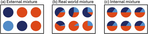
A defining property of an aerosol is that particles are generally mixtures of different organic and inorganic components, as realized by Junge (1952). These mixtures often arise already at the time of emission, and then evolve further as a result of aerosol processes during transport, including gas-particle partitioning, heterogeneous and multiphase reactions, or coagulation. Winkler (1973) stated an important implication concerning a population of particles: The same bulk composition of an aerosol “can be caused by an infinite variety of different internal distributions of the various compounds.” This property is termed the aerosol mixing state. Figure 1 illustrates this concept, with one extreme being the external mixture where each particle only contains one pure compound (Figure 1a), and the other extreme being the internal mixture, where each particle contains a mixture of compounds, with the mass fractions equal to the bulk (Figure 1c). In the ambient atmosphere, the mixing state is in between these two extremes, with an example shown in Figure 1b.

Figure 1. Illustration of the term aerosol mixing state. Each box shows an aerosol population with six particles, with colors representing different chemical species. The populations shown in (a), (b), and (c) have the same bulk composition, but their mixing states differ. (a) External mixture, (b) one of many possible examples of a mixing state in between external and internal mixture, and (c) internal mixture.

In recent decades, there has been a growing realization that mixing state is important for understanding aerosol climate and health impacts, since these impacts depend on per-particle composition in a non-linear way. A good example is the absorption of solar radiation by an aerosol that consists of a non-absorbing species, e.g., ammonium sulfate, and an absorbing species, e.g., black carbon (BC). The absorptivity of the aerosol will be higher when the aerosol is internally mixed compared to the external mixture, even if the species bulk concentrations are the same. This is because the absorptivity of the population is determined by the sum of the absorptivities of the individual particles, and the individual particles’s absorptivity is enhanced for the internally mixed case. The difference can be large enough to matter for radiative forcing calculations, as pointed out already by Jacobson (2001) and Chung and Seinfeld (2002). This has led to efforts to both measure aerosol composition on the per-particle level (Murphy et al. 1998; Middlebrook et al. 2003; Sullivan and Prather 2007; Pratt and Prather 2010; Ault et al. 2010; Bondy et al. 2018), thereby learning about the prevalent mixing state in the ambient atmosphere, and to represent mixing state in models (Riemer et al. 2003; Bauer et al. 2008; Oshima et al. 2009; Riemer et al. 2009; Ching et al. 2016; Matsui et al. 2013; Zhu et al. 2015).

We are now at a point where single-particle data are becoming more and more available, where compute power is sufficient to run mixing-state-aware models, and where new analytical techniques, including machine learning, offer the possibility of processing large amounts of high-dimensional single-particle data to infer population-level properties and processes. Now is the right time to reevaluate how we should be thinking about some of the basic questions in aerosol science to facilitate aerosol model representations and model-measurement comparisons—How should we describe the aerosol state? What are the implications for modeling and measuring aerosols? What does it take to meaningfully compare mixing state measurements with model results?

2. How should we describe the aerosol state?

As aerosol scientists, we are trained to visualize aerosol populations as number, surface, or mass size distributions. This makes sense, given the crucial role that particle size plays for many of the aerosol impacts that we care about, such as the propensity of particles to form cloud droplets and to initiate ice formation, or the ability to scatter and absorb radiation. However, the distribution-based representation is limiting when dealing with an aerosol that has a realistic mixing state somewhere on the spectrum between an internal and external mixture. In that case, it is appropriate to think of the aerosol as a multi-dimensional distribution that resides in a space where the dimension is given by the number of distinct species, called the composition space.

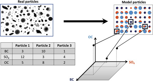
Figure 2 illustrates the example of an aerosol that consists of three species that are commonly represented in models, BC, sulfate (${\text{SO}}_4$), and organic carbon (OC), i.e., forming a three-dimensional composition space. Each particle is defined by a vector $\overrightarrow{\mu }$ that specifies the mass of each species in the particle. The set of vectors from the particles in the population defines the aerosol state. Different aerosol processes acting on these particles cause them to move within the composition space. For example, condensation of secondary organic aerosol would cause the particles to move along the axis labeled with OC, while coagulation of two particles would result in the removal of the two parent particles and the creation of a new particle with a composition vector that is the sum of the parent particles’ composition vectors. In reality, the dimension of the composition space is much higher than three, especially if we consider the multitude of organic components individually, and the additional per-particle properties to capture morphology, charge, and other features. Rather than working with discrete particles, to formulate the governing population balance equations (Riemer et al. 2019), it is convenient to introduce a generalized number distribution $n(\overrightarrow{\mu })$ of an aerosol that contains A species, so that (1) $$n(\overrightarrow{\mu })d{\mu }_{1}d{\mu }_2\dots d{\mu }_A$$(1) is the number concentration of particles where species 1 has mass between ${\mu }_1$ and ${\mu }_1+d{\mu }_1,$ species 2 has mass between ${\mu }_2$ and ${\mu }_2+d{\mu }_2,$ and so forth.

Figure 2. Illustration of the concept of the aerosol state as set of vectors, where each vector describes the composition of one particle. The set of particles can be placed accordingly in the composition space of the aerosol, in this example shown as a three-dimensional space. Microscopy images of real particles courtesy of Miriam Freedman, Pennsylvania State University.

Having established this fundamental way of describing the aerosol state, it is easy to see that our traditional size distributions are a particular choice of one-dimensional projections of the true high-dimensional aerosol state. Importantly, while it is straightforward to construct the low-dimensional projections from the true aerosol state, the reverse is not possible. This means, if we only have information about one-dimensional mass distributions, ambiguity exists regarding the mixing state of the aerosol, or in other words, many different mixing states are consistent with the same one-dimensional mass distribution. This fact introduces uncertainties in our estimates of aerosol-related impacts, such as aerosol-cloud interactions or aerosol-radiation interactions.

3. What are the implications for modeling (and measuring) aerosols?

Several approaches exist to simulate aerosols, with each approach differing in the way that the particle population is represented, namely bulk models, modal models, moment models, sectional models, and particle-resolved models. With the exception of particle-resolved models, these are nothing else than particular low-dimensional projections of the aerosol state as introduced in Section 2, and they are related as shown in Figure 3. Note that even particle-resolved models simplify the true aerosol state since assumptions regarding morphology and shape are made.

Figure 3. Illustration of three different ways the true (high-dimensional) composition space can be collapsed into low-dimensional projections, for bulk, modal, and sectional model representations.

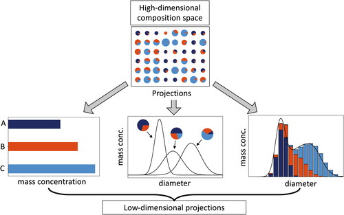
Each type of model makes its specific assumptions about mixing state, which may differ between different representations. Bulk models track the species’ mass concentrations and inherently treat the aerosol as an external mixture of sulfate, BC, OC, sea salt, and dust (Koch 2001; Schult, Feichter, and Cooke 1997; Tegen and Miller 1998).

The underlying assumption of modal models is that the aerosol consists of several overlapping subpopulations (modes), with each subpopulation represented by a log-normal function of the diameter (Whitby and McMurry 1997). Within each mode, an internal mixture is assumed, but since different modes can overlap within a given size range, mixing state can be resolved to a certain extent. This has been exploited to represent the aging process of soot in regional (Riemer et al. 2003) and global models (Koch et al. 2009; Liu et al. 2016), that is, the conversion of soot from its freshly emitted, uncoated state to its aged state after it is coated with secondary aerosol material. While separating “fresh” and “aged” soot into two different modes is closer to reality, it introduces new challenges as threshold parameters need to be set to define what separates fresh and aged modes and how the modes interact, which are difficult to constrain. Furthermore, the internal mixture assumption in the mixed modes leads to biases when optical properties are calculated since the distribution of coating materials on BC cores is not captured correctly (Fierce et al. 2017).

While modal models use several overlapping log-normal functions, sectional models discretize the aerosol size range into a number of sections where each section is assumed to be internally mixed. Consequently, the change of composition with size is resolved, but diversity of composition within a narrow size range is not resolved, unless several one-dimensional bin structures are introduced (Jacobson 2002).

In contrast to modal and sectional models, particle-resolved models resolve composition space by discretely sampling the space with a large number of computational particles. This way, mixing state is inherently resolved, and particle-resolved models can be used to benchmark other aerosol model types with respect to mixing state assumptions. From these exercises, we learn about the magnitude of errors that are introduced when simplifying mixing state assumptions are applied to determine population-level quantities such as aerosol absorption or cloud condensation nuclei (CCN) concentrations. Fierce et al. (2016) showed that it is important to capture the distribution of coatings over a population of BC cores to be able to predict absorption enhancements in line with observations. Ching et al. (2017) found that when internal mixing was assumed, CCN concentrations were up to 100% overpredicted for more externally-mixed populations, but were well predicted for more internally-mixed populations. For mixing states in between internal and external mixture, the errors could remain up to 50%.

Is it not possible to construct a sectional model with a multi-dimensional grid structure? In principle yes, and this has been done for specific choices of two- and three-dimensional grid structures (Oshima et al. 2009; Matsui et al. 2013; Ching et al. 2016). However, beyond this, the curse of dimensionality (Bellman 1957) strikes and higher-dimensional sectional models become too computationally expensive, since the number of bins scales with the number of bins in each dimension to the power of the dimension. Particle-resolved models overcome the curse of dimensionality by placing computational particles only where real particles exist (most of the many bins in high-dimensional sectional models would actually be empty, but still need to be allocated) and by exploiting stochastic sampling techniques.

The projection of composition space to a lower dimension not only occurs in the context of aerosol models; it also applies in the context of aerosol measurements. Measured number and mass size distributions are straightforward examples. Other examples include CCN spectra (one-dimensional projection on supersaturation) or measurements of BC core/coating distributions by single-particle soot photometers (SP2, two-dimensional projection on BC core size and coating thickness). Furthermore, each measurement technique only “sees” a certain sector of composition space, both in terms of the physical particle sizes and in terms of which species can be identified.

4. What does it take to meaningfully compare mixing state measurements with model results?

Not only does aerosol mixing state individually complicate aerosol characterization by measurements and their representations by models; it also challenges the comparison of the two. We are used to comparing measurements and model results of scalar quantities (e.g., species mass concentrations, total number concentrations) or discretized one-dimensional distributions (e.g., number or mass size distributions, CCN spectra). However, comparing mixing state is much more difficult because it requires comparing sampled high-dimensional distributions.

To accomplish this, one can take several approaches, depending on what kind of data is available. For example, in a scenario where model output from a particle-resolved model and single-particle data from an aerosol mass spectrometer are available, one approach could be to directly work in the high-dimensional space, using a Wasserstein metric (Villani 2008) to quantify the distance between the measured and modeled (high-dimensional) distributions. However, a problem with this approach is that it is difficult to establish a clear mapping between the particle-resolved model output (masses of model species in each particle) and the data that a mass spectrometer provides (relative intensities for certain $m/z$ ratios for each particle). Even if this mapping exists, this approach would be difficult to visualize or to interpret.

An alternative is to revert back to low-dimensional projections. Some of these, e.g., mass concentrations or size distributions, do not contain mixing state information. In this case, the comparison can be augmented with a scalar quantity that is sensitive to mixing state, such as the mixing state metric $\chi$ (Riemer and West 2013). This metric is based on species mass fractions in each particle and includes two distinct aspects: how complex individual particles are (in terms of being composed of different species) and how similar different particles are within a population. The metric $\chi$ ranges from 0% for a fully external mixture to 100% for a fully internal mixture and can quantify any state in between. If measurements and model results agree in terms of number and mass size distributions and in terms of mixing state index, this would increase our confidence that the model captures mixing state correctly (Zhu et al. 2016). Using this framework does require the knowledge of quantitative per-particle composition, which is straightforward to determine with a particle-resolved model, but not available for more simplified modeling approaches, and challenging to determine from observational data.

In contrast to mass concentrations or size distributions, other low-dimensional projections do have mixing state information embedded. For example CCN spectra contain information on how species of different hygroscopicity are mixed (Su et al. 2010; Yuan and Zhao 2023). Another example are measurements with the single-particle soot photometer from which distributions with respect to BC core size and coating thickness (or their ratio) can be derived (Matsui et al. 2013). These (partial) measures of mixing state are especially useful if they are applied in a size-resolved manner, so that particle size and mixing state can be disentangled. For a more complete characterization of mixing state, collocated measurements of several different instruments are needed.

5. Conclusions

This editorial elucidates the fundamental properties of the aerosol state and the implications of the fact that atmospheric aerosols are mixtures of mixtures—each aerosol particle usually contains several chemical components, and particles of diverse composition are assembled within a population. A convenient way to conceptualize this fact is to think of the aerosol residing in a high-dimensional composition space. The implications can be summarized as follows:

• Common aerosol modeling approaches and aerosol measurement techniques work with low-dimensional projections of this high-dimensional space. As a result, information of the true aerosol state is lost.

• There are many different ways to obtain low-dimensional projections for use as aerosol model representations. This introduces structural and parametric uncertainties in our models that are to date still largely unquantified.

• Comparisons of mixing state predictions with observations are challenging. One of the main hurdles in this endeavor is to find a mapping between the quantities that the model tracks and the quantities that a given measurement technique provides. Only when such a mapping exists is a quantitative comparison possible.

• It is worth devoting effort to develop such mappings because it will allow for stronger constraints on our aerosol predictions, which are necessary to ensure that we obtain the right results for the right reasons in our predictions of aerosol climate impacts.

Disclosure statement

No potential conflict of interest was reported by the author(s).

Additional information

Funding

This work was supported by NSF award 1941110 and by the Department of Energy Atmospheric System Research program, Office of Biological and Environmental Research, award DE‐SC0022130.

References

- Ault, A. P., C. J. Gaston, Y. Wang, G. Dominguez, M. H. Thiemens, and K. A. Prather. 2010. Characterization of the single particle mixing state of individual ship plume events measured at the port of Los Angeles. Environ. Sci. Technol. 44 (6):1954–61. doi:10.1021/es902985h.
- Bauer, S., D. Wright, D. Koch, E. Lewis, R. McGraw, L.-S. Chang, S. Schwartz, and R. Ruedy. 2008. MATRIX (Multiconfiguration Aerosol TRacker of mIXing state): An aerosol microphysical module for global atmospheric models. Atmos. Chem. Phys. 8 (20):6003–35. doi:10.5194/acp-8-6003-2008.
- Bellman, R. 1957. Dynamic programming. Princeton, NJ: Princeton University Press.
- Bondy, A. L., D. Bonanno, R. C. Moffet, B. Wang, A. Laskin, and A. P. Ault. 2018. The diverse chemical mixing state of aerosol particles in the southeastern United States. Atmos. Chem. Phys. 18:12595–612. doi:10.5194/acp-18-12595-2018.
- Ching, J., J. Fast, M. West, and N. Riemer. 2017. Metrics to quantify the importance of mixing state for CCN activity. Atmos. Chem. Phys. 17 (12):7445–58. doi:10.5194/acp-17-7445-2017.
- Ching, J., R. A. Zaveri, R. C. Easter, N. Riemer, and J. D. Fast. 2016. A three-dimensional sectional representation of aerosol mixing state for simulating optical properties and cloud condensation nuclei. JGR. Atmospheres 121 (10):5912–29. doi:10.1002/2015JD024323.
- Chung, S. H., and J. H. Seinfeld. 2002. Global distribution and climate forcing of carbonaceous aerosols. J. Geophys. Res. 107 (D19): AAC 14-1–AAC 14-33. doi:10.1029/2001JD001397.
- Fierce, L., T. C. Bond, S. E. Bauer, F. Mena, and N. Riemer. 2016. Black carbon absorption at the global scale is affected by particle-scale diversity in composition. Nat. Commun. 7 (1):12361. doi:10.1038/ncomms12361.
- Fierce, L., N. Riemer, and T. C. Bond. 2017. Toward reduced representation of mixing state for simulating aerosol effects on climate. Bull. Am. Meteorol. Soc. 98 (5):971–80. doi:10.1175/BAMS-D-16-0028.1.
- Jacobson, M. Z. 2001. Strong radiative heating due to the mixing state of black carbon in atmospheric aerosols. Nature 409 (6821):695–7. doi:10.1038/35055518.
- Jacobson, M. Z. 2002. Analysis of aerosol interactions with numerical techniques for solving coagulation, nucleation, condensation, dissolution, and reversible chemistry among multiple size distributions. J. Geophys. Res. 107 (D19):4366. doi:10.1029/2001JD002044.
- Junge, C. E. 1952. Die Konstitution des atmosphärischen Aerosols. Ann. Met. 5:1–55.
- Koch, D. 2001. Transport and direct radiative forcing of carbonaceous and sulfate aerosols in the GISS GCM. J. Geophys. Res. 106 (D17):20311–32. doi:10.1029/2001JD900038.
- Koch, D., M. Schulz, S. Kinne, C. McNaughton, J. Spackman, Y. Balkanski, S. Bauer, T. Berntsen, T. C. Bond, O. Boucher, et al. 2009. Evaluation of black carbon estimations in global aerosol models. Atmos. Chem. Phys. 9 (22):9001–26. doi:10.5194/acp-9-9001-2009.
- Liu, X., P.-L. Ma, H. Wang, S. Tilmes, B. Singh, R. Easter, S. Ghan, and P. Rasch. 2016. Description and evaluation of a new four-mode version of the modal aerosol module (MAM4) within version 5.3 of the Community Atmosphere Model. Geosci. Model Dev. 9 (2):505–22. doi:10.5194/gmd-9-505-2016.
- Matsui, H., M. Koike, Y. Kondo, N. Moteki, J. D. Fast, and R. A. Zaveri. 2013. Development and validation of a black carbon mixing state resolved three-dimensional model: Aging processes and radiative impact. JGR. Atmospheres 118 (5):2304–26. doi:10.1029/2012JD018446.
- Middlebrook, A. M., D. M. Murphy, S.-H. Lee, D. S. Thomson, K. A. Prather, R. J. Wenzel, D.-Y. Liu, D. J. Phares, K. P. Rhoads, A. S. Wexler, et al. 2003. A comparison of particle mass spectrometers during the 1999 Atlanta Supersite Project. J. Geophys. Res. 108 (D7):8424. doi:10.1029/2001JD000660.
- Murphy, D., J. Anderson, P. Quinn, L. McInnes, F. Brechtel, S. Kreidenweis, A. Middlebrook, M. Pósfai, D. Thomson, and P. Buseck. 1998. Influence of sea-salt on aerosol radiative properties in the Southern Ocean marine boundary layer. Nature 392 (6671):62–5. doi:10.1038/32138.
- Oshima, N., M. Koike, Y. Zhang, and Y. Kondo. 2009. Aging of black carbon in outflow from anthropogenic sources using a mixing state resolved model: 2. Aerosol optical properties and cloud condensation nuclei activities. J. Geophys. Res. Atmospheres 114:D18202. doi:10.1029/2008JD011681.
- Pratt, K. A., and K. A. Prather. 2010. Aircraft measurements of vertical profiles of aerosol mixing states. J. Geophys. Res. 115:D11305. doi:10.1029/2009JD013150.
- Riemer, N., A. Ault, M. West, R. Craig, and J. Curtis. 2019. Aerosol mixing state: Measurements, modeling, and impacts. Rev. Geophys. 57 (2):187–249. doi:10.1029/2018RG000615.
- Riemer, N., H. Vogel, B. Vogel, and F. Fiedler. 2003. Modeling aerosols on the mesoscale-γ: Treatment of soot aerosol and its radiative effects. J. Geophys. Res. Atmospheres 108:4601. doi:10.1029/2003jd003448.
- Riemer, N., and M. West. 2013. Quantifying aerosol mixing state with entropy and diversity measures. Atmos. Chem. Phys. 13 (22):11423–39. doi:10.5194/acp-13-11423-2013.
- Riemer, N., M. West, R. A. Zaveri, and R. C. Easter. 2009. Simulating the evolution of soot mixing state with a particle-resolved aerosol model. J. Geophys. Res. 114:D09202. doi:10.1029/2008JD011073.
- Schult, I., J. Feichter, and W. F. Cooke. 1997. Effect of black carbon and sulfate aerosols on the Global Radiation Budget. J. Geophys. Res. Atmospheres. 102 (D25):30107–17. doi:10.1029/97JD01863.
- Su, H., D. Rose, Y. Cheng, S. Gunthe, A. Massling, M. Stock, A. Wiedensohler, M. Andreae, and U. Pöschl. 2010. Hygroscopicity distribution concept for measurement data analysis and modeling of aerosol particle mixing state with regard to hygroscopic growth and CCN activation. Atmos. Chem. Phys. 10 (15):7489–503. doi:10.5194/acp-10-7489-2010.
- Sullivan, R. C., and K. A. Prather. 2007. Investigations of the diurnal cycle and mixing state of oxalic acid in individual particles in Asian aerosol outflow. Environ. Sci. Technol. 41 (23):8062–9. doi:10.1021/es071134g.
- Tegen, I., and R. Miller. 1998. A general circulation model study on the interannual variability of soil dust aerosol. J. Geophys. Res. 103 (D20):25975–95. doi:10.1029/98JD02345.
- Villani, C. 2008. Optimal transport: Old and new. New York, NY: Springer.
- Whitby, E. R., and P. H. McMurry. 1997. Modal aerosol dynamics modeling. Aerosol Sci. Technol. 27 (6):673–88. doi:10.1080/02786829708965504.
- Winkler, P. 1973. The growth of atmospheric aerosol particles as a function of the relative humidity—II. An improved concept of mixed nuclei. J. Aerosol Sci. 4 (5):373–87. doi:10.1016/0021-8502(73)90027-X.
- Yuan, L., and C. Zhao. 2023. Quantifying particle-to-particle heterogeneity in aerosol hygroscopicity. Atmos. Chem. Phys. 23 (5):3195–205. doi:10.5194/acp-23-3195-2023.
- Zhu, S., K. N. Sartelet, R. M. Healy, and J. C. Wenger. 2016. Simulation of particle diversity and mixing state over Greater Paris: a model–measurement inter-comparison. Faraday Discuss. 189:547–66. doi:10.1039/c5fd00175g.
- Zhu, S., K. N. Sartelet, and C. Seigneur. 2015. A size-composition resolved aerosol model for simulating the dynamics of externally mixed particles: SCRAM (v 1.0). Geosci. Model Dev. 8 (6):1595–612. doi:10.5194/gmd-8-1595-2015.