The ELPI Response and Data Reduction II: Properties of Kernels and Data Inversion

The first part of this article reports the analytical form of the Electrical Low Pressure Impactor (ELPI) kernel functions. In this latter part, the numerical quality of ELPI response matrices is studied and an example of an inversion algorithm is given. The ELPI assemblies with and without an electrical filter stage and with smooth or sintered impaction plates are studied and compared with basic impactor kernels and the kernels for the calculation of the aerosol mass distribution. It is shown that the ELPI assembly with the electrical filter stage and smooth impaction plates should be the best choice for the inversion of data if no bounce occurs. The comparison to a mass impactor shows that the devices are on par in data inversion. The inversion ELPI data is studied with a Bayesian algorithm assuming a bimodal lognormal size distribution of the aerosol. The algorithm includes a novel procedure for obtaining an initial guess of the distribution parameters. To our knowledge, it is also the first algorithm to use ELPI current readings as its input. Simulations and diesel emission measurements show that the proposed algorithm is a useful tool in the study of ELPI data.

INTRODUCTION

Traditionally, impactor data is treated using the cut diameter concept (e.g., Cooper and Guttrich 1981). This has the merit of conserving all the measured information. For Electrical Low Pressure Impactor (ELPI, Keskinen et al. 1992; Marjamäki et al. 2000; Marjamäki et al. 2002), this concept would display the measured current as a histogram on aerodynamic diameter axis. However, one normally wishes to find either number or mass distribution. This can also be done using the same concept. During the process, the nonideal collection characteristics are taken into account by correcting the measured currents (Moisio 1999). This is already an irreversible process, so that original measurement result cannot be constructed from the corrected distribution. Further, there is a problem in treating the filter stage data, as there is no lower cut diameter to enter the calculation. The problem can be overcome by using an inversion algorithm to obtain the distribution. As a bonus, these algorithms produce a continuous, smooth function for the distribution.

To run an inversion algorithm, the instrument kernel functions need to be known. These were derived for ELPI in the first part of this article (Marjamäki et al. 2005). Generally, the problem can be presented as a Fredholm integral equation of the first kind:

Here y is the output vector of the linear system, z some quantity typical of problem, K(z) the kernel function, that is, a known mapping from real axis to the output vector space and f(z) a distribution function of some quantity related to the problem. A great amount of research has been done on this class of equations (e.g., Twomey 1979, for a good bibliography see Hansen 1998) and several inversion schemes have been presented for gravimetric impactors (e.g., Sundelöf 1967; Raabe 1978; Puttock 1981; Tatsch et al. 1984; Hasan and Dzubay 1987; Wolfenbarger and Seinfeld 1990). One inversion algorithm has been constructed for the ELPI by Dong et al. (2004) but their approach considers the ELPI as a mass impactor ignoring the advantage of the electric measurement, the short measurement period. In addition, their method does not treat the secondary deposition and gives no chance to use the electrical filter stage (Marjamäki et al. 2002) of the ELPI.

It has been noted by many workers (e.g., Cooper and Wu 1990) that with real aerosol measurement devices, small changes in the output greatly affect the inversion result f. This can be attributed either to rank-deficiency or ill-posedness of the problem. It is instructive to study the numerical properties of the ELPI kernel functions as these determine the difficulty met in the inversion and the methods best suited for it.

For ill-posed problems, the traditional concepts of the condition number and the rank are not useful in the description of the numerical properties of the kernel matrix. Instead, we use the degree of ill-posedness and the effective numerical rank. First, singular value decomposition of the kernel matrix is used to analyzed the degree of ill-posedness of the inversion problem. Second, we apply the concept of effective numerical rank to the standard-form Tikhonov regularization.

The weakness of all regularization algorithms is the choice of the regularization parameter. On the other hand, many aerosol size distributions have a uni- or bimodal log-normal distribution. In the final part of this article, we present a Bayesian method to obtain a bimodal log-normal distribution from the measured ELPI raw data, including an automated algorithm to find sui initial values by using the pseudo inverse of the kernel matrix. This algorithm is, to our knowledge, the first to use ELPI current measurement as its input. The method is then tested both by simulations and real measurement data.

Numerical Properties of Response Functions

Using the notation of the first part of this article, the integral in Equation can easily be seen to be the scalar product < E _ch k _i , α^{− 1} D _p ^−β f > in the vector space C[0, ∞). If we define the current vector I = [I ₁,…, I _N ]^T, we can write

where K is the ELPI kernel matrix [E _ch k ₁,…, E _ch k _N ]^T and ϵ is the vector representing random measurement error. In practical applications the integral in Equation 2 must be calculated numerically which requires its discretization. The vectors f and ϵ and the instrument response matrix K now have finite dimensions. If we have m discretization points K∈ R ^{N× m} and f ∈ R ^m .

The inversion of ELPI data can be made to return different distribution types. As pointed out in the first part of this article (Marjamäki et al. 2005), it would be most natural to establish the current distribution (i.e., 1.5th moment distribution). As an inversion problem, this would correspond to the traditional case of gravimetric impactor measurement. The two most widely used distributions are the number distribution (i.e., zeroth moment) and the mass distribution, the third moment. We shall study the difficulty of inversion into all three moments.

The ELPI can be used in several configurations. The impactor can be assembled with or without the electrical filter stage (Marjamäki et al. 2002) and the impactor stages can have smooth or sintered impactor plates. The kernel functions for each case are different. In addition, two alternative ways of ELPI data inversion were studied. In the first situation, the response matrix not multiplied by the charger efficiency was studied. This represents roughly the 1.5th moment of the number distribution. At the same time, the impactor kernel functions of the ELPI represent those of a traditional impactor. This setting gives a possibility to compare the ELPI with a similar 12-stage mass impactor, which is an extremely well-known instrument. In the second alternative, the mass distribution was calculated from the simulated currents. As discussed by Keskinen et al. (1992), the charger efficiency functions and the impactor kernel functions depend on different size concepts. Therefore, the overall kernel matrix is dependent on particle density which was assumed to be 1.000 kg/m³. As another simplification, space charge deposition was neglected, which would correspond to low concentration measurement.

The basic equations and methods needed in applying the concepts of ill-posedness and effective numerical rank are reviewed in the appendix. The degree of ill-posedness is determined solely from the instrument response matrix and is not dependent on the problem. In Figure 1, the singular values of K are shown for the three different moment distributions. It is evident that in all the cases, they are well fitted by equation:

where α is the degree of ill-posedness of the kernel matrix. This makes the inversion problem of the ELPI ill-posed (Hansen 1998, p. 8). Values of α are given in Table 2. The degree of ill-posedness is least in the case of an ELPI equipped with smooth plates and the filter. Although the pure impactor response function is also best fit by Equation 3, its singular values are all of the same magnitude, which is mirrored by a very low degree of ill-posedness. Hence the problem cannot actually be considered ill-posed in this case. The degree of ill-posedness for the mass distribution kernel is not very much higher than for the number distribution kernels. The situation is well illustrated by Figure 1.

Figure 1 The logarithms of the singular values of the response matrix for the ELPI with an electrical filter stage. It is easy to see that the best degree of ill-posedness is achieved when making an inversion to the current distribution. The kernel for the mass distribution is slightly more ill-posed than the kernel for number distribution.

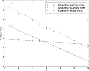
Table 2 Degrees of ill-posedness and effective numerical ranks for various ELPI make-ups

Degrees of ill-posedness and effective numerical ranks
		Effective numerical ranks
ELPI make-up	Degree of ill-posedness ^a	Distr. 1	Distr. 2	Distr. 3	Distr. 4 ^b	Distr. 5
Noiseless measurement
Filter, smooth plates	0.682	11.76	12.00	11.95	3.35	12.00
Filter, sintered plates	0.801	11.36	11.36	11.96	0.28	12.00
Std., smooth plates	0.797	11.71	12.00	11.95	3.35	12.00
Std., sintered plates	0.800	11.37	11.37	11.95	0.28	11.37
Std., smooth, no charging	0.096	11.92	12.00	12.00	0.004	12.00
Std., smooth, calculating mass	0.780	12.00	0.29	0.29	0.29	0.29
Noise 5%
Filter, smooth plates		10.97	10.63	11.93	3.09	10.74
Filter, sintered plates		9.86	9.54	11.78	0.28	10.07
Std., smooth plates		11.04	10.63	11.93	3.35	10.94
Std., sintered plates		10.01	9.72	11.81	0.28	9.90
Std., smooth plates, no charging		11.59	11.71	11.62	0.004	11.70
Std., smooth, calculating mass		12.00	0.29	0.29	4.97	0.29

The numerical properties of the response functions were studied according to the following scheme: Tikhonov regularization was run on error-free, simulated ELPI measurement data from four different size distributions. All distributions were log-normal and multimodal. The effect of noise was taken into account in the next phase, where random noise with a standard deviation of 5% of the respective channel current was added to the simulated data. This models the ELPI measurement error quite well. Distribution I was unimodal, distribution 2 bimodal, and distribution 3 had three modes. These distributions were composed of same peaks so that distribution 2 included the peak from distribution 1 and distribution 3 the peaks from the distributions 1 and 2. Distribution 4 was practically monodisperse, with a geometric standard deviation of 1.05. Distribution 5 was distribution 2, the CMDs of the modes of which were reversed. It might be argued that the use of the size distribution makes the inversion of distributions with a more concentrated mode of small particles easier than the inversion of distributions where the large particles are dominant. With such distributions, it might be better to use, for instance, the moment 1.5 which corresponds the kernel functions with the charger neglected. The purpose of distribution 5 was to check whether such phenomenon occurs. The data for the distributions is in Table 1.

Table 1 Modes of the distributions used to study the numerical properties. The exact value of N is not significant as the space charge deposition is neglected. A linear problem, the inversion uses only relative values

	Included in
Peak	distributions	N (arb.axis)	CMD/μ m	GSD
I	1,2,3	1	0.2	1.5
II	2,3	0.5	2	1.3
III	3	3	0.02	1.6
IV	4	1	0.3	1.05
V	5	1	2	1.3
VI	5	0.5	0.2	1.5

For each distribution and every response function, the regularization parameter was sought producing the best fit between the inversion output and the input distribution. The parameter values were then used to calculate the effective numerical rank values shown in Table 2. The maximum possible effective numerical rank value is equal to the number of measurement channels, or 12. A lower value corresponds to a higher degree of regularization (see Appendix). The lower the value, the more difficult is the inversion problem. The results were encouraging. With the normal kernel matrices, even so simple an algorithm as Tikhonov regularization manages to fit the three modes of distribution 3. The effective numerical rank increases as the distributions become broader, reflecting the fact that the particles are deposited more evenly on the stages. With the distribution 3, an extremely broad, trimodal distribution the modes of which can well be distinguished, the effective numerical rank of all instrument compositions is close to 12. For the other distributions, it can be seen that with a noiseless measurement, information could be extracted also from the stages on which only secondary deposition is significant. With noisy measurements, however, the quality of data decreases and the amount of information is reduced. The broad distribution 3 still retains its good qualities. The comparison of the effective numerical ranks in the cases of distributions 2 and 5 does not reveal any significant difference between situations where the median diameters of the modes have been swapped. The narrow distribution 4 reminds us that the Tikhonov regularization has its shortcomings, as it failed to fit a function to it with all response functions, regardless of the parameter choosing method applied. This is reflected by the very low effective numerical ranks for this distribution. It must be noted that the algorithm later described also failed to give any inversion result for the data simulated for this distribution, returning an error instead.

Although the effective numerical rank is defined only for individual problems, we can make conclusions from the data. It is visible that the effective numerical ranks in the problems with the porous plates are consistently inferior to the problems with smooth plates. This obviously results from the lesser steepness of the impaction curves mentioned by Marjamäki and Keskinen (2004). The inferiority of the porous plates with ill-defined cut points is beautifully consistent with the traditional impactor analysis but in the case the filter stage, the analyses differ. The degree of ill-posedness of the instrument response matrix of the ELPI with filter and smooth impaction plates is clearly lower than that of other the ELPI compositions. The ELPIs with a filter also have effective numerical ranks comparable to ones without a filter. This leads one to think that the inversion of data from an ELPI with a filter need not be any more difficult than the inversion of data from one without it. This is not the case with the traditional impactor analysis, which suffers from the ill-defined cut points of the filter. In addition, it is encouraging to see that the kernel matrix for number distribution of the ELPI assembly with smooth plates and an electrical filter stage is not significantly worse with the data inversion than the “chargerless” kernel function. The inversion to the mass distribution seems much more difficult, however. Standard Tikhonov inversion fits only the unimodal distribution well, totally failing with the other distributions using any inversion parameter value. For these distributions, the effective numerical ranks become quite low.

Inversion of Bimodal Log-Normal Distribution

In contrast to the application described in the previous section, the input size distribution is not known in real inversion problem. This brings up the weakness of the regularization algorithms, the choise of the regularization parameter. Even with a parameter choice algorithm, the number of modes in the final inversion result may be subject to human influence. On the other hand, many aerosol size distributions have a uni-or bimodal log-normal distribution. For instance, when measuring diesel emissions, one knows almost surely that the aerosol size distribution has an accumulation mode and an eventual nucleation mode. In such a situation, one can safely assume a functional form for the distribution. This will also reduce the distribution into a concise form suitable for applications such as modeling.

There are several procedures to fit a set grouped data into a bimodal log-normal size distribution—a size distribution vector in our notation. These have been discussed and compared by de Ruiter and Oeseburg (1987). However, they implicitly assume that the particle sizes are correctly measured which limits the use of their results. Ramachandran and Kandlikar (1996) propose a Bayesian inversion method for cascade impactor data. They discuss the inversion of Personal Inhalable Dust Spectrometer (PIDS) data but their method can readily be applied to any cascade impactor. They apply the Bayesian method for the inversion of a bimodal log-normal size distribution but find their a prioriinformation by manual, traditional impactor analysis. Although straightforward and reliable, this method is ill suited for automated algorithms. In addition, they use only five independent parameters, as the total mass is measured directly by weighing. With the ELPI, this cannot be done. It is the number concentration that is studied in the inversion and the implementation of the total current as a constraining parameter makes the inversion algorithm unwieldy. Therefore, we characterize the bimodal size distribution

by six parameters: Total concentrations of the modes (N ₁, N ₂), their geometric mean diameters d _g1, d _g2 and the geometric standard deviations (GSD) σ _g1 and σ _g2. The use of weighing factors γ_i of the modes,

to diminish the number of independent variables is not done during the inversion. However, the weighing factors simplify the description of a distribution. As the working of the inversion algorithms described below is independent of the exact magnitude of the impactor currents, the distributions used in simulation are best described by the use of weighing factor γ₁.

The Bayesian approach to the problem is simple and outlined by Ramachandran and Kandlikar (1996). Let us denote the vector containing the six parameters of the bimodal lognormal distribution by θ ∈ V where V is the set of physically acceptable values of θ. The probability of the size distribution θ producing the current vector I is

Here P(I) is the probability of measuring current vector I, P(I/θ) is the probability to measure current vector I if the distribution is θ and P ₀(θ) is the a priori probability of the distribution θ.

The probability of receiving the result I _i from the measurement of the “true” current of I′ _i′ on the impactor stage i is the probability of measuring current I _i with distribution θ.

Here we have assumed the currents to be normally distributed which seems to be the case with the ELPI. σ _i is here the standard deviation (SD) of the current i. We assume, like Dzubay and Hasan (1990), the standard deviation to have a constant component from the background noise and a varying component that is proportional to the current on the channel:

The units of the parameters σ _i and σ_c are here amperes (or, more likely, femtoamperes), the parameter σ_v being a pure number. This approach is perhaps too simple because it does not take the effect of other channels into account. However, as there is no data on the dependency of the error of ELPI currents on the current on different channels, this simple approach should be sufficient.

If the errors of the currents from impactor plates are assumed independent, the probability of measuring the current vector I is

The probability of measuring current vector I is simply

where V is the set of the allowed values for parameter vector θ.

There is no reason to believe that one distribution should be more probable than another within the set V. Therefore it is logical to assume P ₀(θ) to be constant. When we substitute 9 and 10 to Equation 6, we get

Both algorithms give the most probable value, that is, the expectation value of θ as their result. When we use the Latin Hypercube sampling method, the estimate for this is given by

As Ramachandran and Kandlikar (1996) point out, this is likely to give the lowest residuals. The ‘random design method’ mentioned by De Ruiter and Oeseburg (1987) is reminiscent of the method outlined above but the final result θ is the value minimizing or maximizing a given error function.

The a Priori Values

The method proposed above requires some a priori knowledge of possible distributions to limit the space V of the allowed parameters. Ramachandran and Kandlikar (1996) use values obtained by manual analysis. De Ruiter and Oeseburg (1987) mention the use of computer algorithm to find the a priori values but dismiss it as undependable. Anyhow, if we are to make an automatic inversion procedure, we cannot rely on manual procedures and must resort to a computer algorithm. A feasible set of initial values can be obtained by using the pseudoinverse K ⁺ of the kernel matrix. A rough estimate of the distribution, which itself might be a suitable inversion result for many purposes, is received from

The received vector is sought for maxima. The highest maximum is likely to be in the vicinity of the count mean diameter (CMD) of a mode. Finding the other mode is more difficult because the ELPI kernels cause oscillation of f _guess and there may be several “artificial” maxima on the downward slopes of the first mode. In addition, the second mode often appears only as a “shoulder” of the distribution. Luckily, the modes of this kind can still produce a minimum due to oscillation caused by the kernels. The problem, however is the most difficult as the two modes are close to each other and cannot be easily resolved from the data even with trained eye. Although the human eye can usually easily distinguish the second mode, a reliable algorithm is harder to construct. We demand arbitrarily that the f _guess must have a minimum of less than 60% of its maximum value between the first and the second mode maxima. This is done to prevent the irrelevant oscillation from causing a virtual mode in the vicinity of the first maxima. The obvious draw-back is the fact that two modes very close to each other will be considered one even when a trained eye would see the difference.

Another way to construct the two maxima would be to use some regularization algorithm but this is not rational. If we use a regularization algorithm, there should be no need for the Bayesian algorithm afterward.

The initial guess of the total number of a mode is the total number of particles with size below (or above) the aforementioned minima. Because the real-world aerosol mode almost always has a geometric standard deviation (GSD) of 1.2–2, this is taken to be the range for the GSD of both modes. This limits the applicability of the algorithm but those atmospheric aerosols that do have a GSD above 2 often have more than two modes. The count median diameters and total number concentrations of both modes are assumed to lie between 60% and 140% of their initial guesses.

RESULTS

The algorithm was tested in two phases. First a set of simulated data was studied with the algorithm. In the second part of the study, the algorithm was used for the inversion of laboratory measurement data. In the simulations, four distributions were studied. Distribution A models a diesel exhaust aerosol with a nucleation (typical size range 1–70 nm) and a soot mode (typical size range 50–500 nm). Distribution B does not have an exact counterpart in nature but models a situation in which the two modes are close to each other. Distribution C is the second distribution used in the study of the numerical properties of impactor kernels. It can be considered to resemble a power plant emission aerosol with a coarse mode (typical size range 1–10 μm) and an accumulation mode (soot 50–500 nm). Distribution D, which is composed of the more concentrated peak of distribution B, demonstrated the working of the algorithm in case of unimodal input. The data for the distributions is given in Table 3.

Table 3 The distributions used to study the proposed inversion procedure

	Distribution	Distribution	Distribution	Distribution
	A	B	C	D
d g1 (μ m)	0.015	0.2	0.2	0.2
d g2 (μ m)	0.083	0.4	2	—
σ g1	1.3	1.3	1.5	1.5
σ g2	1.6	1.5	1.3	—
g1	0.91	0.75	0.67	1

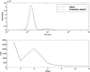
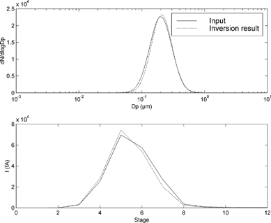
The distributions were tested by running the inversion algorithm on the simulated ELPI measurement currents. To bring the simulations closer to a real measurement, a random error, the standard deviation of which was 5% of each channel current, was added to the simulated current values. The algorithm functioned satisfactorily. The inversion error seems to be largest with the peaks near the lower limit of the ELPI measurement range—below 30 nm. This is mirrored by the result from the inversion of distribution I (Figure 2). The mode with a diameter of 10 nm is collected mainly on the electrical filter stage the response function of which is quite flat. However, the charger efficiency decreases rapidly in this size range. Therefore, the inversion problem has two solutions: a mode with a relatively low number concentration and a larger median diameter causes almost the same current measurement as a mode with a higher concentration and a smaller CMD. This is, however a property of the ELPI response functions, not a failure of the inversion algorithm.

Figure 2 The result of the inversion of distribution A. Above, the number distributions of the distribution and its inversion result are depicted. The simulated ELPI currents from the both distributions are shown below. It is remarkable to see how a modest error in the number concentration of the second mode causes a large error in the simulated currents while a quite large error in the first mode causes almost no error in the simulated currents.

The distributions B, C, and D give good inversion results. (Figure 3 Figure 4 Figure 5). The relative standard deviations of the parameter components θ _i in the output are smaller than the relative error of the channel currents. In case of a unimodal distribution, the algorithm tries to produce a bimodal distribution to fit the measurement data from the unimodal one. This typically results in a two peaks. The number concentration of the smaller peak is typically circa 5% of the concentration of the larger one and the peaks overlap almost completely. This is well exemplified by Figure 5, where the second “mode” cannot be distinguished although the algorithm reports parameters for it. The goodness of the fit can also be estimated quite well by comparing the “measured” current to the one simulated from the inversion result.

Figure 3 The inversion result of distribution B. The graphs as in Figure 2. It is quite ramerkable how well the algorithm has been able to fit the function although two distinct peaks are not visible.

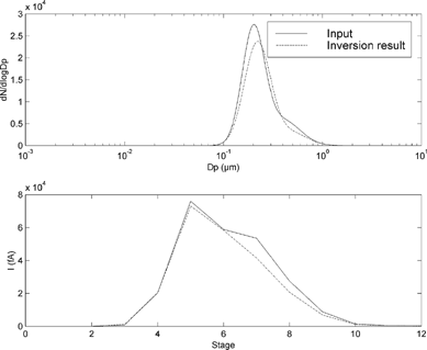
Figure 4 The inversion result of distribution C. The graphs as in Figure 2.

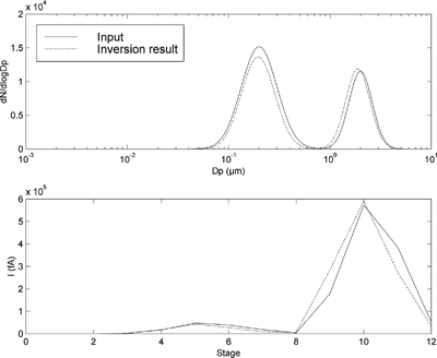
Figure 5 The inversion result of distribution D. The graphs as in Figure 2.

The practicability of any inversion algorithm can only be estimated by the inversion of real measurement data. For this purpose, we studied actual diesel engine measurement data. The emission was simultaneously measured with an ELPI and two Scanning Mobility particle sizers (SMPS): a TSI nano-SMPS and a TSI SMPS with a long DMA (Knutson and Whitby 1975; Wang and Flagan 1990). The emission was diluted by a factor of 12 before measurement. The ELPI was fitted with smooth impactor plates and an electrical filter stage. The data used for inversion is a mean of 50 individual ELPI measurements. As the diesel engine running at constant power is a quite stable aerosol generator, the aerosol distribution can be considered constant during an SMPS scan. This enables us to use the SMPS measurement as the “correct” form of the aerosol size distribution. Nevertheless, the exact flow rates of the instruments can differ from the calibration values which could cause a systematic error to the situations. If there always is a constant error of 10% between the SMPS and ELPI measurements, it is unfair to demand the algorithm to produce inversion results resembling the SMPS measurement data. This problem can be circumvented by normalizing the distributions:

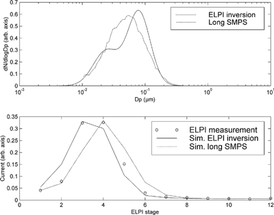
The inversion of the experimental data succeeds quite well. Typical output is presented in Figure 6 Figure 7 Figure 8. The number distribution estimated by the ELPI software, SMPS measurements and the ELPI inversion result fit each other quite well. The inversion can even estimate the “tail” of the distribution quite well. In other cases where the nucleation mode is smaller and its CMD is below 10 nm, the inversion does not fit the data quite as well as in Figure 6. In the case of unimodal data (Figure 8), the inversion produces an unrealistic shoulder. This is caused by the faulty a priori values given by the initial guess algorithm. As the simulations show, the initial guess algorithm succeeds much better when the only mode has a CMD of 200 nm. Therefore, the tendency to produce an unnecessary second mode is present only when the filter stage receives significant current. It need be noted that the calculation of ELPI kernels requires knowledge of particle density. With the experimental data, the density of particles was assumed to be 0.8 gcm^{− 3}. The discussion of the effect of particle density and eventual fractal properties of the aerosol particles on the inversion of ELPI data is beyond the scope of this paper.

Figure 6 An example of the inversion of a diesel emission distribution. Both the number distributions and the current distributions are normalized. Above, the number concentrations from the inversion procedure, from the long and the short SMPS are presented. Below, the measured ELPI currents and the simulated currents from the inversion result and the SMPS scans are shown. The comparison of simulated and measured currents shows that the inversion has succeeded quite well. The difference between the currents is at largest on the filter stage.

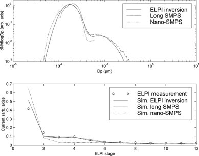
Figure 7 An example of the inversion of a diesel emission distribution. Figures as in Figure 6. In this case, the SMPS and inversion result number concentrations agree so well that there is no need for normalization. The comparison of simulated and measured currents shows that the nucleation mode generated by the algorithm is larger than the measured currents allow. The difference between the currents is at largest on the lowest impactor stage.

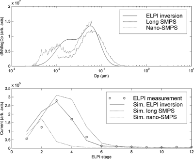
Figure 8 An example of the inversion of a diesel emission distribution. Figures as in Figure 6. The inversion produces a “shoulder” that has no counterpart in reality. However, this can be detected by comparing the simulated current of produced by the inversion result with the actual measurement. This kind of behavior, which results form a bad initial values, was not detected with unimodal distributions the CMD of which was at least 200 nm.

The previously described algorithm was ineffective when used with the kernel matrix for the mass distribution. However, a fit to the unimodal mass distribution is possible. This is consistent with the effective numerical ranks of the ELPI kernel matrix for the mass distribution.

DISCUSSION

The object of this paper has been to analyze the numerical properties of the response matrices of different ELPI combinations and to demonstrate the suitability of the matrices for the inversion of the ELPI data. The numerical properties of the ELPI impactor were analyzed with methods that to our knowledge have not been previously used in aerosol science. However, we believe that the concepts of numerical rank and degree of ill-posedness might bring some quantitative aspects to the discussion of the difficulty of inversion. For example, the concept of degree of ill-posedness allows us to say exactly that the inversion problem of the ELPI data is severely ill-posed. The concept of numerical rank shows quantitatively that the inversion of data from an ELPI with an electrical filter stage should be about as difficult as the data inversion of an ELPI without one. It can also be seen that there is no significant disadvantage in the inversion of ELPI data compared to the inversion of traditional mass impactor data. We can also state, that with reasonably broad size distributions, even 9–11 parameters can be assigned to depict the size distribution with a good hope of extracting them from the ELPI measurement data.

The moment of the distribution that is given as the output of an inversion procedure has a significant effect on the difficulty of inversion. From the degrees of ill-posedness of different kernels we can see that the most natural quantity used as the ELPI measurement output would be the current distribution. However, the study of the effective numerical ranks shows that the inversion into the number distribution is not significantly inferior. On the other hand, the inversion into mass distribution should be much more difficult to construct which was later seen. ELPI kernel matrix for this case does not have a much higher degree of ill-posedness than the normal kernel matrices but the corresponding effective numerical ranks are mostly quite low. It might be inferred that the degree of ill-posedness is not very good indicator of the difficulty of data inversion. It seems that ELPI inversion algorithm giving number distribution as its output should make the best compromise between usefulness and numerical ease.

We must not lose the sight of the physical measurement and its inaccuracies. Although we might ponder that an ELPI with porous impaction plates is less suited for data inversion than the otherwise same ELPI with smooth plates, the inaccuracy of response matrix is not visible in mathematical modeling performed above. The porous plates, for instance, reduce the particle bounce, which is only qualitatively understood yet. In some cases, this will make them more suitable for many measurements regardless of their potential inferiority in mathematical sense.

In addition to an analysis of the numerical properties of the ELPI kernel functions, we demonstrated their use in the inversion by applying them to the case of bimodal lognormal size distribution. The inversion procedure itself is the one applied by Ramachandran and Kandlikar (1996) to the Personal Inhalable Dust Spectrometer (PIDS, Gibson et al. 1987) but the initial guess is made by a novel algorithm. The fact that the inversion result is not the same quantity as the measurement data causes some difficulty that is usually not present in aerosol inversion problems. With simulated and experimental number distributions, the algorithm performed satisfactorily but was unsuccessful in returning a mass distribution. However, a fitting procedure for a unimodal mass distribution could be constructed following the same lines.

The assumption that the size distribution has a clear functional form can be criticized strongly because no real aerosol obeys a particular size distribution. Nonetheless, we believe that the use of functional form has the advantage of sincerity: as we make a conscious assumption of the form of the size distribution function, we admit our preconceptions. After this, the algorithm runs determinedly. While using a more general algorithm, the researchers are easily inclined to run the inversion procedure with different parameter choices so long that the inversion result is satisfactory. In addition, the algorithm assuming a functional form returns the parameters of the distribution, which may be helpful in understanding the nature of the aerosol studied.

The use of inversion requires care. The workers should be well acquainted with the aerosol studied by inversion and they should consider the results critically. In addition, as ELPI kernels depend on the density of the particles measured, this should be well known. The success of the inversion is best estimated by comparing the measured currents with the ones simulated from the inversion result. If these do not fit reasonably well, it is best to consider the inversion unsuccessful. It is also worthwhile to compare the measured currents with the noise. It is not useful to report “modes” that may well be artifacts generated from the noise.

CONCLUSIONS

The study of the effective numerical ranks of the ELPI kernels shows that a number distribution is not too difficult to obtain from the ELPI data. The mass distribution is much more difficult. The actual usability is demonstrated with the inversion procedure of Ramachandran and Kandlikar (1996) which was modified to be fully automatic. The results from the numerical study are reinforced when the algorithm is applied to the simulated data. A bimodal lognormal number distribution is relatively well fit while the same procedure can determine only a unimodal mass distribution.

The ELPI inversion was applied on real data from diesel emission measurements and the results compared with simultaneous SMPS measurements. It appears that the inversion of the ELPI data is practicable and the algorithm proposed can be used with real measurement data.

ACKNOWLEDGMENTS

The data used in this article was measured as a part of projects LIPIKA (Fine particles from traffic and their relation to laboratory test measurements) and Liquid Particles: Effect of After Treatment Systems and Lubricating Oil, funded by the National Technology Agency (TEKES), Ministry of Transport and Communications of Finland, Ecocat Oy, and Neste Oil Oyj. We thank Mr Topi Rönkkö and Ms. Kati Vaaraslahti for the permission to use their data. We also thank Dr. Arto Voutilainen of University of Kuopio for his advice and suggestions.

Notes

^a Degree of ill-posedness does not depend on noise.

^b Effective numerical rank is low due to failed standard Tikhonov regularization.

APPENDIX: DEGREE OF ILL-POSEDNESS AND EFFECTIVE NUMERICAL RANK

The singular value decomposition provides tools to study the nature of a linear problem quantitatively. The singular value decomposition decomposes the matrix K into three components:

The number of nonzero singular values r is the rank of the matrix K.

In the case of a useful inversion problem, the number of data points wanted from the inversion must necessarily be smaller than the number of ELPI channels, so N ≥ m. The rank of the matrix is the number of non-zero singular values. However, the instrument matrix is a measurement result and therefore noisy. The numerical rank r _ϵ tells the minimum number of linearly independent rows in the case that K is changed with any matrix E, ‖ E‖ ≤ ϵ,

In case of the matrix norm

where the vector norm used is Euclidean, the numerical rank is the number of singular values for which σ _i ≥ ϵ. If the problem is simply rank-deficient, there are two kinds of singular values: large and small and the choice of ϵ is easy. If the problem is ill-posed the singular values are distributed in a more continuous fashion and there is no reason to place ϵ between any two particular singular values. In such case, the concept of numerical rank may be replaced with the concept of degree of ill-posedness (e.g., Hansen 1998, p. 8). In case of mildly or moderately ill-posed problems the singular values comply approximately with the relationship

in which α is the degree of ill-posedness. The problem is severely ill-posed when

(Hansen 1998, pp. 8–9.)

The concept of numerical rank can be introduced into the realm of ill-posed problems with some modification. In order to do this, Tikhonov regularization (Tikhonov 1963) need be introduced. The Tikhonov regularization, as all regularization algorithms, strives to eliminate the ill-posedness of the inverse problem by adding on some extra information. In the basic variation of Tikhonov regularization, the following formula is minimized:

in which f _λ is the regularized solution related to λ. This sets extra cost for unrationally high peaks present in the wild oscillation due to too low λ. The general form of Tikhonov regularization allows for better side constraints and usually gives better results, but for the present purpose, the basic form suffices.

Tikhonov regularization can be seen as a procedure in which the effects of the lowest singular values are filtered out. The strength of the filtering of the singular value σ _i is depicted by filter factor

The filter factors are always connected with the regularization parameter λ. We choose to study the filter factors with λ_opt—the parameter value returning the best fit in the Tikhonov regularization. The sum of filter factors is obviously closely connected with the concept of rank, so it is fitting to call the sum

effective numerical rank. In general form Tikhonov regularization, the filter factors can also be defined and a different effective numerical rank established, but for the purposes of this study, Equation 22 should suffice (e.g., Hansen 1998, 73, 178).

There are several possible ways to define the best fit and in this study, we choose to use definition

In real measurements, f _true can never be known so this definition confines the study of numerical effective rank to simulated data.

REFERENCES

- Cooper , D. W. and Guttrich , G. L. 1981 . A Study of the Cut Diameter Concept for Interpreting Particle Sizing Data . Atm. Env. , 15 : 1699 – 1707 .
- Dong , Y. , Hays , M. D. , Smith , N. D. and Kinsey , J. S. 2004 . Inverting Cascade Impactor Data for Size-Resolved Characterization of Fine Particulate Source Emissions . J. Aerosol Sci , 35 ( 12 ) : 1497 – 1512 . [CROSSREF]
- Dzubay , T. G. and Hasan , H. 1990 . Fitting Multinormal Lognormal Size Distributions to Cascade Impactor Data . Aerosol. Sci. Technol. , 13 : 144 – 150 .
- Gibson , H. , Vincent , J. H. and Mark , D. 1987 . A Personal Inspirable Dust Spectrometer for Applications in Occupational Hygiene Research . Ann. Occ. Hyg , 31 : 463 – 479 . Referred to by Ramachandran and Kandlikar 1996[CSA]
- Hansen , P. C. 1998 . Rank-deficient and discrete ill-posed problems: Numerical aspects of linear inversion , Philadelphia : SIAM .
- Hasan , H. and Dzubay , T. G. 1987 . Size Distributions of Species in Fine Particles in Denver Using a Microorifice Impactor . Aerosol Sci. Technol. , 6 : 29 – 39 . [CSA]
- Keskinen , J. , Pietarinen , K. and ja Lehtimäki , M. 1992 . Electrical Low-Pressure Impactor . J. Aerosol Sci. , 23 : 353 – 360 . [CROSSREF]
- Knutson , E. O. and Whitby , K. T. 1975 . Aerosol Classification by Electric Mobility: Apparatus, Theory and Applications . J. Aerosol Sci. , 6 : 443 [CROSSREF]
- Lekhtmakher , S. and Shapiro , M. 1999 . Short communication on the paper “Inverse methods for analyzing Aerosol Spectrometer Measurements: A Critical Review,” . J. Aeros. Sci. , 31 ( 7 ) : 867 – 873 . [CSA] [CROSSREF]
- Marjamäki , M. , Ntziachristos , L. , Virtanen , A. , Ristimäki , J. , Keskinen , J. , Moisio , M. , Palonen , M. and Lappi , M. 2002 . Electrical filter stage for the ELPI . SAE paper 2002-01-0055
- Marjamäki , M. and Keskinen , J. 2003 . Effect of Impaction Plate Roughness and Porosity on Collection Efficiency . J. Aerosol Sci , 35 ( 3 ) : 301 – 308 . [CROSSREF]
- Marjamäki , M. , Lemmetty , M. and Keskinen , J. 2005 . ELPI response and data handling I: Response functions . Aerosol Sci. Tech , submitted for
- Moisio , M. 1999 . Real time size distribution measurement of combustion aerosols PhD Thesis. Tampere University of Technology
- Puttock , J. S. 1981 . Data Inversion for Cascade Impactors: Fitting Sums of Log-Normal Distributions . Athmos. Environ. , 15 ( 9 ) : 1709 – 1716 . [CROSSREF]
- Raabe , O. G. 1978 . A General Method for Fitting Size Distributions to Multicomponent Aerosol Data Using Weighted Least-Squares . Envir. Sci. Technol. , 12 : 1162 – 1167 . [CSA] [CROSSREF]
- Ramachandran , G. and Kandlikar , M. 1996 . Bayesian Analysis for the Inversion of Aerosol Size Distribution Data . J. Aeros. Sci , 27 ( 6 ) : 1099 – 1112 . [CROSSREF]
- Sundelöf , L. 1967 . On the Accurate Calculation of Particle Size Distributions in Aerosols from Impaction Data . Staub Rainhalt. Luft , 27 : 22 – 28 .
- Tatsch , C. E. , Yeager , W. M. and Johnson , G. L. 1984 . PADRE: A Computerized Data Reduction System for Cascade Impactor Measurements . JAPCA , 34 ( 6 ) : 655 – 660 .
- Tikhonov , A. N. 1963 . Solution of Incorrectly Formulated Problems and the Regularization Method . Soviet Math. Dokl. , 4 : 1035 – 1038 . English translation of Dokl. Akad. Nauk. SSSR 151:501–504 Referred to by Hansen 1998
- Twomey , S. 1979 . Introduction to the mathematics of inversion in remote sensing and indirect measurements , Amsterdam : Elsevier .
- Virtanen , A. , Marjamäki , M. , Ristimäki , J. and Keskinen , J. 2001 . Fine Particle Losses in Electrical Low Pressure Impactor . J. Aerosol Sci , 32 : 389 – 401 . [CSA] [CROSSREF]
- Wang , S. C. and Flagan , R. C. 1990 . Scanning Electrical Mobility Spectrometer . Aerosol Sci. Technol. , 13 : 230 – 240 .
- Wolfenbarger , J. K. and Seinfeld , J. H. 1990 . Inversion of Aerosol Size Distribution Data . J. Aerosol, Sci. , 2 : 227 – 247 . [CROSSREF]