Model-based investigation on the effects of spatial evenness, and size selection in thinning of Picea abies stands

ABSTRACT

Size and spatial distribution of trees are important for forest stand growth, but the extent to which it matters in thinning operations, in terms of wood production and stand economy, has rarely been documented. Here we investigate how the choice of spatial evenness and tree-size distribution of residual trees impacts wood production and stand economy. A spatially explicit individual-based growth model was used, in conjunction with empirical cost functions for harvesting and forwarding, to calculate net production and net present value for different thinning operations in Norway spruce stands in Northern Sweden. The in silico thinning operations were defined by three variables: (1) spatial evenness after thinning, (2) tree size preference for harvesting, and (3) basal area reduction. We found that thinning that increases spatial evenness increases net production and net present value by around 2.0%, compared to the worst case. When changing the spatial evenness in conjunction with size preference we could observe an improvement of the net production and net present value up to 8.0%. The magnitude of impact differed greatly between the stands (from 1.7% to 8.0%) and was highest in the stand with the lowest stem density.

KEYWORDS:

• Thinning
• individual-based model
• spatial distribution
• forest management
• simulation

Introduction

Thinning operations produce fewer trees, but with larger diameters, and promote the production of merchantable timber, thereby increasing the value of the stand (Wallentin 2007; Nilsson et al. 2010). Moreover, since the removed trees are recovered, thus preventing self-thinning, the net wood production is higher in the thinned stands (Nilsson et al. 2010). Hence, thinning has a positive effect on a stand’s net production and net value (Valsta 1992a; Zeide 2001; Hyytiäinen and Tahvonen 2003; Cao et al. 2006). However, thinning can be carried out in many ways, in terms of the multiple choices regarding which trees to remove. Some common terms for describing thinning prescriptions are basal area reduction, tree size preferences, and spatial evenness. At stand level, the effect of basal area reduction is well known (Zeide 2001; Mäkinen and Isomäki 2004; Wallentin 2007; Nilsson et al. 2010), just as it is known that the removal of smaller trees (i.e. thinning from below) marginally increases net production (Nilsson et al. 2010). Increased spatial evenness has shown a potential for increased net production (Baldwin et al. 1989; Mäkinen et al. 2006).

What has not been fully addressed is how basal area reduction, tree size preferences (thinning form) and spatial evenness interrelate, and how significant an effect each of them has on net production if other aspects are kept constant. Moreover, from an economic perspective, it could be argued that the rise in income from the increased net production and wood value does not compensate for the increase in harvesting costs. Due to the long rotation time and time-consuming field measuring, such experiments are difficult to perform empirically.

However, the experiments can be addressed using a model-based approach. Indeed, so-called individual-based models (IBMs) (Grimm and Railsback 2005) can be used. IBMs use information on a tree-by-tree basis and simulate interaction between the trees to predict the future growth of each individual tree, e.g. Pacala et al. (1996), Liu and Ashton (1998), Phillips and Gardingen (2001), Seidl et al. (2012), Cronie et al. (2013). IBMs have been used in a variety of studies such as identifying thinning regimes on an individual tree level in order to minimise the risk of forest fire (Contreras 2010; Contreras and Chung 2013) and studies of forest management in which the timber price and growth are stochastic (Valsta 1992b; Pukkala 2015). To our knowledge, IBMs have not been used to address the question of the effect of spatial evenness and thinning form.

In this study, we analyse how different spatial distributions, after thinning operations, in conjunction with different thinning intensities, and thinning forms, affect the net present value and net production of the stand during an entire rotation. To achieve this, we developed an individual-based model, in which both tree diameter and height growth were modelled and applied asymmetric distance-dependent competition between all individual trees. The model has been fitted and validated against data from an experimental Norway spruce (Picea abies) forest in Northern Sweden.

Material and methods

Overview

In the model used for the study, the development of a forest stand after a single thinning was simulated for the stand’s full rotation period, with evaluation of the effects from variations in how the thinning was performed. The stand’s rotation time was split into three phases: (1) thinning phase, (2) growth phase and (3) clear-cut phase (Figure 1). The simulation started at the initial stand age $t_0$ (years), at which all trees with a diameter at breast height over bark ($\mathrm{DBH}$) of less than 8 cm were removed in order to simulate a removal of hindering undergrowth. Next, but still under year $t_0$, a commercial thinning was performed. The selection of trees to be removed was determined by the specified thinning procedure, based on a different emphasis on three criteria: (1) spatial evenness after thinning, (2) tree size preference for trees to remove and (3) basal area reduction. The volume and value of the removed trees were calculated (but not for trees removed as hindering undergrowth, i.e. with a $\mathrm{DBH}<8\mathrm{cm}$). Costs for both the thinning and undergrowth removal were calculated, assuming that the operation was conducted using Nordic cut-to-length machines (harvester and forwarder).

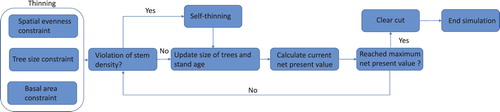
Figure 1. Overview of modelling procedure. At the start of each simulation, an algorithm is used to identify a selection of trees to be removed in an initial thinning operation. The selection is chosen such that the pre-set conditions for spatial evenness after thinning, the thinning ratio, and basal area after thinning are fulfilled. The selected trees are removed from the stand and the growth simulation starts. In each simulation step the growth of all remaining individual trees in the stand is calculated and the stand age is increased. If the mean diameter in the stand surpasses the maximum mean diameter, for the given stand density, self-thinning occurs, and tress are removed. The growth simulation ends when the maximum net present value of the stand is reached, at which the remaining trees are removed in a clear-cut and the simulation ends.

At the start of the growth phase, the maximum mean diameter that could be sustained by the current stand density was calculated in order to assess if self-thinning would commence. Next, the annual increment in $\mathrm{DBH}$ and height for each tree in the stand was calculated based on a growth model that considered the distance-dependent competition between all trees. The size of each individual tree was updated, the net present value for the stand was calculated for a rotation length equal to t₀, and the stand age was increased by one year. This procedure with growth and net value calculations was repeated until the maximum net present value was reached. This initiated the clear-cut phase, in which the volume, value and costs of a final felling at the given stand conditions were calculated. Besides the net present value of the stand, the mean net production was also calculated as the sum of the harvested timber volume (i.e. not including undergrowth removal or self-thinning) divided by stand age at the time of the clear-cut. The model, with the variations in thinning criteria, was applied to different initial stand configurations, based on data from field measurements. The effects of the different emphasis on thinning criteria were evaluated based on the total net production and the total net value of the stands.

Spatial explicit growth model

We use an IBM to simulate the growth of each individual tree in the initial plot. Let $N_T$ denote the number of trees in the stand. Let $I=\{1,2,\cdots N_T\}$ be a set of indices, and let each individual tree in the stand be uniquely associated with one index from $I$. The dynamics of diameter at breast height (cm), $\mathrm{DB}{\mathrm{H}}_{i,t}$, for each individual tree $i$ at age $t$, is modelled as a modified logistic growth function as in Kot (2001) see (1).(1) $\mathrm{\Delta }\mathrm{DB}{\mathrm{H}}_{i,t}=r\cdot \mathrm{DB}{\mathrm{H}}_{i,t}\cdot max\left(1-\frac{\mathrm{DB}{\mathrm{H}}_{i,t}+CI(i,\mathbf{D}\mathbf{B}{\mathbf{H}}_t,\mathbf{D}\mathbf{i}\mathbf{s}\mathbf{t},\mathit{\theta })}{\mathrm{DB}{\mathrm{H}}_{max}},0\right).$(1) Here $\mathrm{\Delta }\mathrm{DB}{\mathrm{H}}_{i,t}$ is the annual diameter increase, and $r$ and $\mathrm{DB}{\mathrm{H}}_{max}$ are positive-valued model parameters. $r$ is the growth rate of the tree and $\mathrm{DB}{\mathrm{H}}_{max}$ is the maximum $\mathrm{DBH}$, a tree can obtain in the absence of competitors. CI is the competition index function (2). Let $\mathbf{D}\mathbf{B}\mathbf{H}$ be the set of diameters for all trees, i.e. $\mathbf{D}\mathbf{B}\mathbf{H}=\{\mathrm{DB}{\mathrm{H}}_1,\mathrm{DB}{\mathrm{H}}_2\cdots ,\mathrm{DB}{\mathrm{H}}_i,\cdots ,\mathrm{DB}{\mathrm{H}}_{N_T}\}$. $\mathbf{D}\mathbf{i}\mathbf{s}\mathbf{t}$ is the set of all pairwise distances between the trees in the stand, i.e. $\mathbf{D}\mathbf{i}\mathbf{s}\mathbf{t}=\left\{\mathrm{dis}{\mathrm{t}}_{i,j}\right|i\ne j,i,j\in I\}$, where $\mathrm{dis}{\mathrm{t}}_{i,j}=\sqrt{{(x_i-x_j)}^2+{(y_i-y_j)}^2}$, and the ordered pair $(x_i,y_i)$ denotes the position along the x- and y-axis of tree i. $\mathit{\theta }$ is the set of parameters for the competition index function, $\mathit{\theta }=\{\alpha ,\beta ,\lambda \}$. The competition index (CI) models the interaction between the subject tree $i$ and its nearest neighbours. $\mathrm{\Delta }\mathrm{DB}{\mathrm{H}}_{i,t}$ denotes the annual diameter increment for the tree $i$ at age $t$. In our work we use a modified version of the crowding competition index (Canham et al. 2004),(2) $CI(i,\mathbf{D}\mathbf{B}\mathbf{H},\mathbf{D}\mathbf{i}\mathbf{s}\mathbf{t},\mathit{\theta })=\sum _{j\in I\setminus \left\{i\right\}}{\lambda }_{}{\left(\mathrm{DB}{\mathrm{H}}_j/\mathrm{DB}{\mathrm{H}}_i\right)}^{\alpha }\mathrm{dis}{\mathrm{t}}_{i,j}^{-\beta },$(2) as a proxy for the competition pressure that the subject tree is exposed to by its closest neighbours. We define closest neighbours as the neighbours located in a radius of 8 m from the subject tree. The stand is mirrored eight times around the original stand. All individual trees in the mirrored stands are the same size as the corresponding trees in the original stand and the relative distances are also preserved. This is carried out in order to deal with edge effects.

The annual tree height increment (m/year), denoted $\mathrm{\Delta }H$, is modelled as a power law relation to the diameter increment, as follows (3).(3) $\mathrm{\Delta }{H}_{i,t}=\gamma (\mathrm{\Delta }\mathrm{DB}{\mathrm{H}}_{i,t}{)}^{\delta }.$(3) Here, $\gamma ,\delta$ are parameters.

Stem tapering and volume

To calculate the value of the harvested logs, the volume and tapering of the stem were used. Stem tapering and volume were modelled using the tree form function of Edgren and Nylinder (1949) and the volume (in m³), $\mathrm{Vol}$, was calculated as the rotation volume of the tapering function. For further information see the appendix. The diameter at any height of the stem and volume was calculated as a function of the total height of the tree, $\mathrm{DBH}$, and the age of the tree. Further information is provided in the appendix.

Net production and stand economy

We quantify the performance of a given thinning procedure as the net production and net present value of the stand on a per hectare basis. The net production was calculated as the sum of the volume harvested during the thinning operation and the clear-cut, divided by the rotation time (i.e. stand age at the clear-cut). The total value of the stand was determined as the net present value of the stand, in Swedish krona (SEK) ha⁻¹, which was calculated as the sum of the net present value of all three simulated operations (4).(4) $\begin{array}{rl}{V}_{\mathrm{Net}}& =e^{-\ln (1+IR)\cdot t_0}{V}_{\mathrm{pre}-\mathrm{thinning}}+e^{-\ln (1+IR)\cdot t_0}{V}_{\mathrm{thinning}}\\ & +e^{-\ln (1+IR)\cdot T}{V}_{\mathrm{clearcut}}.\end{array}$(4) In (4), $IR$ is the interest rate, which we assume to be 2%, $t_0$ denotes the age of the stand at the start of the simulations, $V_{\mathrm{pre}-\mathrm{thinning}}$ is the value (or rather the cost) of the pre-commercial thinning, $V_{\mathrm{thinning}}$ and $V_{\mathrm{clear}-\mathrm{cut}}$ is the value of the thinning and clear-cut, respectively, at the time they are conducted, calculated according to (5). Here, $T$ denotes the optimal rotation time of the stand.

$T$ was defined as the point in time when the income increment, due to size growth, no longer outweighs the cost increase. If we fixate the thinning procedure (R, TR, and basal area reduction) and initial time for thinning, then an optimal clear-cut is performed when the increase in clear-cut value (not the present value) falls below $\ln (1+IR)$, mathematically: $d{V}_{\mathrm{clear}-\mathrm{cut}}/dt<\ln (1+IR)\Rightarrow d{V}_{Net}/dt<0$; if not, then the net present value will decrease with time.

$V_{\mathrm{pre}-\mathrm{thinning}}$ is assumed to be −2,000 SEK ha⁻¹, whereas $V_{\mathrm{thinning}}$ and $V_{\mathrm{clear}-\mathrm{cut}}$ were determined as the difference between the value of trees removed and the harvesting and forwarding costs (5).(5) $\begin{array}{rl}V=& \sum _{i=1}^{N_R}\left[p\left(\mathrm{DB}{\mathrm{H}}_i\right)\mathrm{Vo}{\mathrm{l}}_i-c_{\mathrm{Harvesting}}\left(\mathrm{Vo}{\mathrm{l}}_i\right)\mathrm{Vo}{\mathrm{l}}_i\right]\\ & -c_{\mathrm{Forwarding}}(\mathrm{Vo}{\mathrm{l}}_{\mathrm{perarea}},\mathrm{Vo}{\mathrm{l}}_{\mathrm{tot}},\mathrm{Vo}{\mathrm{l}}_{\mathrm{mean}})\mathrm{Vo}{\mathrm{l}}_{\mathrm{tot}}.\end{array}$(5)

In (5), $N_R$ is the number of trees selected for removal, $p\left(\mathrm{DB}{\mathrm{H}}_i\right)$ is the DBH-specific price for the tree $i$, $\mathrm{Vo}{\mathrm{l}}_i$ is the stem volume of tree $i$, $c_{\mathrm{Harvesting}},c_{\mathrm{Forwardning}}$ is the cost for the harvester and forwarder operations, respectively. $\mathrm{Vo}{\mathrm{l}}_{\mathrm{tot}}$ is the total volume harvested (m³), and $\mathrm{Vo}{\mathrm{l}}_{\mathrm{perarea}}$ is the mean harvested volume per area (m³ ha⁻¹), and $\mathrm{Vo}{\mathrm{l}}_{\mathrm{mean}}$ is the mean stem volume (m³) of the removed trees in the stand. Hence, the value of a removed tree is determined by its diameter and volume at the time of harvest, as well as by the accumulated volume of all trees removed.

Harvesting costs are calculated on an individual tree basis, through multiplying the tree volume dependent cost per m³ (SEK m⁻³) by the stem volume of the tree (in (5)). To calculate the cost per m³ for a given stem volume in thinning (6) and in clear-cut (7), the fixed hourly cost of the machine was divided by the machine’s tree volume dependent productivity. The hourly cost of the harvester was set to 1,000 SEK h⁻¹ and equations from Nurminen et al. (2006) were used to calculate the harvester’s productivity (m³h⁻¹) as a function of the stem volume (Vol).

Forwarding costs are calculated on a stand level, by dividing the hourly cost of the machine by the average machine productivity in the stand in thinning (8) and in clear-cut (9). The hourly cost of the forwarder was set to 900 SEK h⁻¹. Models by Eriksson and Lindroos (2014) were used to calculate the average forwarding productivity in the modelled stands. However, the following parameters were assumed and were the same for all modelled stands: mean extraction distance = 420 m, adjustable load space = 0, load capacity = 12 m³ for thinning and 16 m³ for final felling, terrain roughness = 1.7, slope = 1.7.(6) $\begin{array}{rl}{c}_{\mathrm{Harvesting},\mathrm{thinning}}\left(\mathrm{Vol}\right)& =1000/(0.383+135.896\mathrm{Vol}\\ & -180.065\mathrm{Vo}{\mathrm{l}}^2),\end{array}$(6) (7) $\begin{array}{rl}{c}_{\mathrm{Harvesting},\mathrm{clearcut}}\left(\mathrm{Vol}\right)& =1000/(4.067+78.623\mathrm{Vol}\\ & -18.507\mathrm{Vo}{\mathrm{l}}^2),\end{array}$(7) (8) $\begin{array}{rl}& c_{\mathrm{Forwarding},\mathrm{thinning}}(\mathrm{Vo}{\mathrm{l}}_{\mathrm{perarea}},\mathrm{Vo}{\mathrm{l}}_{\mathrm{tot}},\mathrm{Vo}{\mathrm{l}}_{\mathrm{mean}})\\ & =900/\exp [2.550+0.074\ln (\mathrm{Vo}{\mathrm{l}}_{\mathrm{perarea}})\\ & +0.046\ln \left(\mathrm{Vo}{\mathrm{l}}_{\mathrm{tot}}\right)+0.259\ln \left(\mathrm{Vo}{\mathrm{l}}_{\mathrm{mean}}\right)],\end{array}$(8) (9) $\begin{array}{rl}& c_{\mathrm{Forwarding},\mathrm{clearcut}}(\mathrm{Vo}{\mathrm{l}}_{\mathrm{perarea}},\mathrm{Vo}{\mathrm{l}}_{\mathrm{tot}},\mathrm{Vo}{\mathrm{l}}_{\mathrm{mean}})\\ & =900/\exp [2.392+0.094\ln (\mathrm{Vo}{\mathrm{l}}_{\mathrm{perarea}})\\ & +0.058\ln \left(\mathrm{Vo}{\mathrm{l}}_{\mathrm{tot}}\right)+0.176\ln \left(\mathrm{Vo}{\mathrm{l}}_{\mathrm{mean}}\right)]\end{array}$(9)

Definition of spatial evenness and emphasis on size.

We use the Clark-Evans nearest neighbour index (R) (Clark and Evans 1954; Leopold et al. 1985) as a measure for spatial evenness. The measure is defined as the ratio between mean distance to nearest neighbour and the expected mean distance to nearest neighbour in a random distribution, see (10).(10) $R=\frac{{\sum }_{i=1}^{N_T}{r}_i}{\overline{r}{N}_T}.$(10) Here, $r_i$ is the distance to the nearest neighbour, for the tree $i\in I$, $N_T$ is the number of trees in the stand and $\overline{r}$ is the expected mean distance to the nearest neighbour in a random distribution. We account for edge effects by using the edge-corrected estimation of $\overline{r}$, described by Sinclair (1985), see (11).(11) $\overline{r}=0.5\sqrt{A/N_T}+(0.051+0.041/\sqrt{N_T})L/N_T.$(11)

In (11), $A$ is the stand area and $L$ is the circumference of the stand. A value of R = 1 means the given spatial distribution is indistinguishable from a random distribution. For R > 1 the distribution is more uniform (even) and for R < 1 the distribution is aggregated (uneven).

We use thinning ratio (TR) as a measure for the preferred size distribution. TR is defined as the ratio between the mean diameter of the removed trees ($\mathrm{DB}{\mathrm{H}}_{\mathrm{Re}}$) and the mean diameter of the remaining trees ($\mathrm{DB}{\mathrm{H}}_{\mathrm{AT}}$), see (12).(12) $TR=\frac{\mathrm{DB}{\mathrm{H}}_{\mathrm{Re}}}{\mathrm{DB}{\mathrm{H}}_{\mathrm{AT}}}.$(12) When TR is equal to 1 it implies that the selection of individual trees is even, in terms of size; this implies that equal numbers of smaller and larger trees were selected. A value larger than 1 implies that predominantly larger trees were selected for removal (thinning from above). Consequently, a value lower than 1 implies an emphasis on removing smaller trees (thinning from below). In our simulations, we vary TR between 0.8–1.2 and R between 0.9 and 1.3.

Self-thinning

In order to account for self-thinning, we implement the algorithm outlined by Pukkala et al. (1998). At the start of a growth period, the mean diameter, $dg$ (cm) is calculated. Using (13) (Elfving 2010), we calculate the maximum number of stems per hectare, $N_{max}$, which can be sustained for the given mean diameter.(13) $\ln \left(N_{max}\right)=12-1.5\ln \left(dg\right).$(13)

If the current stem density is larger than $N_{max}$, trees are removed until the stem density is lower than $N_{max}$. The probability of survival for each tree determines which trees will be removed. Based on the survival function from Pukkala et al. (2013), the trees with the lowest probability of survival are removed first.

Tree selection

To identify a selection of trees to harvest, such that the requirements on the target thinning ratio (TR_Target) and spatial evenness (R_Target) and basal area reduction (BA_Target) are fulfilled, we employ a Monte Carlo Markov Chain (MCMC) method, namely the Metropolis—Hastings algorithm (Gilks et al. 1996). The algorithm starts from an initial guess (an initial tree selection) and updates this guess. The guess is updated in such a way that it “moves” towards the selection which best fulfils the thinning targets. However, with the pre-set values for R_Target, TR_Target, and BA_Target, the final selection of trees will not be unique, i.e. there is more than one selection that fulfils the requirements. The algorithm produces a sample (a collection of different tree selections) with values for spatial evenness, thinning ratio and basal area reduction sufficiently close to R_Target, TR_Target, and BA_Target. For some combinations of R_Target, TR_Target, and BA_Target there is no tree selection fulling the defined requirements, i.e. some combinations of thinning ratio, spatial evenness, and basal area reductions were impossible to achieve. For each sample point (for each tree selection), we calculate V_net and the final performance value associated with the particular thinning operation as the mean net value, ${\overline{V}}_{\mathrm{Net}}$. The algorithm is outlined in more detail in the appendix.

Data for model fitting

The data used in our study are taken from the experimental study area of Flakaliden, in Västerbotten, Northern Sweden (64°07’N, 19°27’E). The main purpose of the site was to study the potential growth of a Norway spruce stand, when it is not limited by nutrients, under the typical climate conditions of that area. In 1963, four-year-old Norway spruces were planted. The experiment started in 1986. By this time, the site had a density of 2,400 stems per hectare, the mean height was 2 m, and the mean DBH was 3.6 cm. At the end of the experiment, it was estimated that the stand would possess a dominant height of 18 m at a stand age of 100 years (site index G18), for the untreated forest area. The experimental site was divided into 33 equally-sized plots, with a dimension of 50 m × 50 m. In each parcel different treatments were applied, such as nitrogen and wood ash fertilisation, solid fertilisation, irrigation with liquid fertilisation, and control zones in which no treatments were applied. In the irrigation treatment, the area was watered daily if the soil-water potential was below a certain threshold from June–August. The solid fertilised plots were given the same amount of nutrients as in the liquid fertilised case, as a one-time application each year. From 1986 to 2013, individual trees were measured approximately every 2–4 years. The dimensions measured were diameter at breast height and tree height. However, tree height was only measured for around 20 sample trees per hectare in all plots. Coordinates for all trees in each plot are known. In 2003, thinning operations were carried out in selected fertilised plots, in which 30% and 60% of the basal area was removed. See Bergh et al. (1999) for further information on the dataset.

Data for modelling – initial stand data

The data for the initial stand is taken from a study in which detailed data from plots selected to represent forest stands at the time of the first commercial thinning operation were collected (Bredberg 1972). Among other data, height, diameter and the coordinates of each individual tree in the stand were recorded. For our simulations we wanted data for pure spruce stands, a condition met by four stands, which consequently were used the simulations. Overview data for the selected stands are given in Table 1. Table 2 shows the stand characteristics after pre-commercial thinning (after removing trees with DBH < 8 cm). In our simulations, we assume all trees in the stands to be spruce trees.

Table 1. Initial plot characteristics.

Stand	Basal area [m^2 ha^−1]	Age [year]	Number of stems per ha	Mean diameter [cm]	Mean Height [m]	Dominant height [m]	Stand area [ha]	Proportion Pine/Spruce/Broad-leaf (% of trees)	Start R-value
GA_502	31.2	33	2,470	12(3.6)	12.7(2.2)	16.7	0.1	0/99.6/0.4	1.22
GA_601	33.8	29	2,200	13.3(4.3)	12.9(2.8)	17.5	0.1	0/96.3/3.7	1.25
GA_602	33.0	25	2,860	12(3.2)	11.3(2.1)	14.8	0.1	0/99.6/0.4	1.33
GA_604	35.3	26	3,360	11(3.6)	11.3(2.2)	16.2	0.1	0/98.8/1.2	1.43

Note: Standard deviation for diameter and tree height are given in parenthesis.

Table 2. Stand characteristics after pre-commercial thinning.

Stand	Basal area [m^2/ha]	Number of stems per ha	Mean diameter [cm]	Mean Height [m]	Start R-value
GA_502	30.1	2,190	12.9(3.3)	13.1(1.7)	1.21
GA_601	32.9	1,930	14.3(3.7)	13.7(2.1)	1.26
GA_602	31.5	2,450	12.5(2.6)	11.9(1.5)	1.31
GA_604	32.5	2,610	12.2(3.2)	12.1(1.7)	1.37

Note: Standard deviation for diameter and height are given in parenthesis.

Fitting and validation of growth model

We used the data from the stand subjected to liquid fertilisation to fit and validate our model. We chose these plots because they include data for thinned and non-thinned stands. The data were divided into two parts: one part is used for the model fitting and the other for model validation. Plots with no thinning, and with 30% and 60% thinning intensity were represented in both sets. For the diameter increment model, the fitted model parameters are depicted in Table 3. The simulated diameter and heights and the actual data are compared in Figure 2.

Figure 2. The diameter model explains 93% of variation. Results from fitting and validation of DBH model and tree height model. All pictures show simulated model data against actual data. (a)-(b) shows the result from the fitting of the DBH and height model. For (a) MSE = 0.38 R² = 0.97 and for (b) MSE = 8.7 R² = 0.58. (c)–(d) shows the results from the validation of the fitted models (DBH model and tree height model, respectively). For (c) MSE = 0.44 R² = 0.93 and for (d) MSE = 8.0 R² = 0.57.

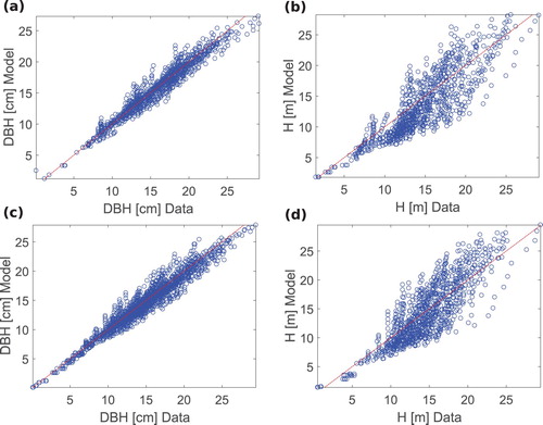
Table 3. Model parameters from fitting.

Model parameter	Value
Diameter increment model
rSpruce [annual^−1]	0.067
DBHMax,Spruce [cm]	35
Competition index
λSpruce [m^β cm^−(α−1)]	0.42
α [-]	0.43
β [-]	1.4
Height increment model
γ [m annual^δ−1 cm^−δ]	0.64
δ [-]	0.57

Note: These are used for all simulations.

Simulation cases

We divide the simulation studies into three cases to study different aspects: spatial evenness, thinning ratios, and thinning ratio and spatial evenness in conjunction.

Case 1: Here we study the effect of spatial evenness on net production and net present value. We set the thinning ratio to 1 and the values for spatial evenness tested were 1, 1.2, and 1.4. Basal area reductions tested for were 30% and 50%.

Case 2: Similar to case 1 but with the focus now on thinning ratios. We test for the thinning ratios 0.8, 1, and 1.2. The R-value is set to 1.2 and the basal area reductions tested for were 30% and 50%. Beside these cases, we also simulate the unthinned case.

Case 3: In the final simulation case we study how changing the R-value and TR-value in conjunction will increase the net production and net present value. We vary the R-value from 0.7 to 1.3 and the TR-value from 0.9 to1.6; the basal area reductions were set to 30%. For every initial stand, we record the lowest value in regard to net production and net present value. The increase is measured as the percentage increase in relation to the lowest values.

Results

Higher spatial evenness increases net production and stand economy

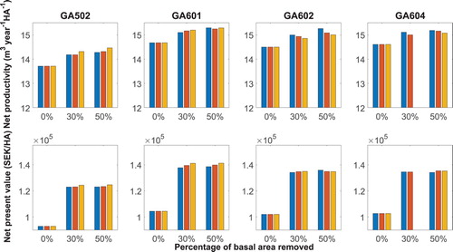
From the results of simulation case 1 we observe that the net production increase with the spatial evenness (see Figure 3), e.g. for initial plot GA502 we observe an increase from 14.2 m³year⁻¹ha⁻¹ to 14.5 m³year⁻¹ha⁻¹, when increasing the spatial evenness (R-value) from 1.0 to 1.4. The mean net production increase was 2% for all plots when the spatial evenness was increased from 1.0 to 1.4. As with net production, the net present value also rises with spatial evenness. The largest increase we could detect was for the initial plot GA604, with a basal area reduction of 50%, where the net present value increased from 132,000 SEK ha⁻¹ to 137,000 SEK ha⁻¹ (r value changes from 1 to 1.4). The mean net present value increase for all plots was 2.5%.

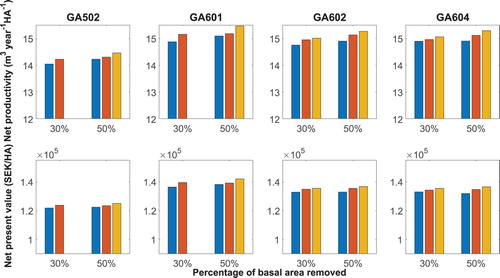
Figure 3. Net production and net present value increase with spatial evenness. The figure depicts the stand economy and net production response to change in basal area reduction and spatial evenness. The basal area is reduced by 30% and 50%. The target thinning ratio (TR) was set to 1 and the spatial evenness was set to 1 (blue bar), 1.2 (red bar) and 1.4 (yellow bar). Results for GA502 and GA601, with spatial evenness set to 1.4 and basal area reduction set to 30%, is missing because no tree selection could be found to fulfil these conditions.

Optimal thinning ratio varies with initial stand characteristics

Simulation case 2 shows that thinning increases net production for all initial plots (Figure 4), e.g. from 13.7 m³year⁻¹ha⁻¹ when no thinning is carried out (basal area reduction 0%) to 14.3 m³year⁻¹ha⁻¹ for the initial plot GA502. If we look at the difference between a thinning intensity of 30% versus 50%, we can only observe a marginal difference. While net production consistently increased, the maximum relative increase was only 1.8%. There was no obvious trend between various thinning ratios, i.e. if a higher or lower thinning ratio results in better net production. For instance, in GA502 (14.3 m³year⁻¹ha⁻¹ for TR 0.8 vs 14.5 m³year⁻¹ha⁻¹ for TR 1.2), thinning from above is superior while in GA602 (15.3 m³year⁻¹ha⁻¹ vs 15.0 m³year⁻¹ha⁻¹), we see the opposite trend. However, the actual difference between the thinning ratios for a given basal area reduction is low; in most cases, less than 1% and at most around 2%. We observe similar trends for the net present value, that thinning substantially improves the net present value but with little effect from thinning intensity or thinning ratio. The difference between non-thinned and thinned stands was substantial, e.g. for GA502 the net present value increases from 93,000 SEK ha⁻¹ if not thinning to 120,000 SEK ha⁻¹ when thinning, meaning an increase of 30%.

Figure 4. Thinning increases net production and net present value. The figure illustrates how the net present value and net production for the different initial stands change with basal area reduction and thinning ratio. The target spatial evenness (R) was set to 1.2, the thinning ratio was set to 0.8 (blue bar), 1 (red bar) and 1.2 (yellow bar), and the basal area reduction was set to 0%, 30% and 50%, respectively. The first row depicts the net production and the second row shows the corresponding net present value. Results for GA602, with thinning ratio 1.2 and basal area reduction of 30%, is missing because no tree selection could be found to fulfil these conditions.

Optimal choice of size and evenness emphasis can increase net production and present value by 8%

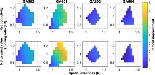
From the results above, we can see that changing thinning ratio or spatial evenness has an impact on the overall stand performance, i.e. net production and stand value. The results from simulation case 3 (see Figure 5) show that the maximum increase in mean net production and net present value are 5.7% and 8.0%, respectively. The maximum increase varies among the different initial plots, e.g. for plot GA502, the maximum increase of net production was around 4.1%, 8.0% for GA601, 2.1% for GA602 and 1.7% for GA604. The general trend is: higher thinning from above (higher thinning value) – and spatial evenness result in greater performance. However, just as in simulation case 2, there are exceptions.

Figure 5. We get a maximum increase of 8% in net production and net present value by changing the thinning ratio and spatial increment. The colours indicate the relative increase in net production and net present value respectively, for a given pair of R- and TR-values, compared to the lowest value. The relative increase is given as a percentage increase. White means no tree selection could be found that satisfied the thinning criteria. The basal area reduction is set to 30%. The thinning ratio(TR) varies from 0.7 to 1.3, and spatial emphasis(R) from 0.9 to 1.6.

Optimal rotation time increases with increased thinning ratio and decreases with spatial evenness

In regard to the optimal rotation time, the results from case 3 show that the timing varies between the different stands: the rotation time varies from 70 years to 80 years (Figure 6). As thinning from above increases, so does the optimal rotation time (Figure 6). The optimal rotation time decreases slightly with spatial evenness.

Figure 6. Optimal timing for clear-cut increases with thinning ratio. The figure shows the time of the optimal clear-cut (year), in terms of stand net value, depending on the selected thinning ratio (TR) and target spatial evenness (R) after thinning. The basal area reduction is set to 30%. t₀ denotes the stand age at the thinning.

Discussion and conclusion

From our simulation work, we found that increased spatial evenness after thinning will improve the net production and net present value of the stand. With regard to the thinning ratio, we could not identify a clear trend. Depending on the initial stand, a higher thinning ratio (thinning from above) would result in higher net production and net present value, while for other initial stands a lower thinning ratio (thinning from below) would be the better choice. When holding the basal area reduction constant and varying the thinning ratio and spatial evenness in conjunction, we found that we could achieve an improvement of 8%, in relation to the worst case, in net production and net present value. We found that the optimal rotation time increased with increased spatial evenness and thinning ratio.

From the results, we can see that a higher spatial evenness, after thinning, will improve the overall performance of the stand. This means that for a given stand density, the mean distance to the nearest neighbour should be high, i.e. trees should be kept in even spatial patterns. This will promote net production and stand economy and is perhaps not surprising. A higher spatial evenness means that, on average, we expect an increase in distance to the nearest neighbour, which also results in more space for most trees. However, it should be noted that if the distance to nearest neighbour is too high (i.e. low stand density), it could negatively impact the wood quality, e.g. increased branching, and productivity (Wallentin 2007). Mäkinen et al. (2006) conducted an empirical comparison between selected thinning (more spatially even) and systematic thinning (less spatially even) at the same thinning intensity for stands of Scots pine and Norway spruce. They found that the net production was lower for the systematic thinning treatment, which agrees with our findings. However, they reported that the difference was small.

In our simulation, we found no consistency regarding whether a lower or higher thinning ratio (i.e. thinning from below or above) would result in higher net production. Overall, the maximum increase was less than one percent for a given basal area reduction, indicating that all selected thinning ratios result in equal production. Empirical studies have reported that thinning from below results in higher net production (e.g. Mielikäinen and Valkonen 1991), since self-thinning increases following a thinning from above (Nilsson et al. 2010). Besides the thinning ratio, we can clearly infer that thinning has a positive impact on net production; a thinning procedure will recover volumes that would otherwise be lost in self-thinning. This is in agreement with what other studies have reported, e.g. Nilsson et al. (2010). However, other studies have found the net production to be highest for unthinned Norway spruce stands, e.g. Mäkinen and Isomäki (2004). In most of the simulation results, thinning from above resulted in the highest net present value, due to higher income in the initial thinning procedure as mainly larger trees are removed. This is in agreement with results from other studies (e.g. Hyytiäinen et al. 2004). When looking at stand economy, the different thinning ratios result in minor changes in net present value. However, the difference between thinned and non-thinned stands was greater (around 30%), reaffirming the well-established knowledge that thinning has a positive impact on stand economy (e.g. Hyytiäinen et al. 2004; Wallentin 2007). When changing the proportion of basal area reduction (within the 0%–50% range), we see only minor changes in both net present value and net production.

Looking at optimal rotation time, spatial evenness appear to have only a minor impact on optimal rotation time. However, a small trend can be detected: an increase in spatial evenness will decrease the rotation time. This is because of the increase in net production. For the thinning ratio, we can see a clearer trend, in which the optimal rotation time increases with the thinning ratio. This is because a higher thinning ratio means that mainly larger trees are removed, resulting in a longer growth period for the residual trees, before reaching the critical threshold.

Although we established that changing spatial evenness and the thinning ratio will alter overall net production and consequently the value of the stand, the maximum improvement varies greatly among the different initial plots. For a given basal area reduction (30% for our simulations), we obtain a maximum increase in net production and the net present value of 5.8% and 8.0%, respectively (Figure 5), for initial plot GA502. In contrast, for plot GA604, the maximum improvement was 2.1%. Thus, our chosen thinning variables impact net production and net present value, but the magnitude of improvement depends on the initial stand characteristics. From the four selected initial plots, we can see a difference between GA502 and GA601, which had the highest increase (4.1% and 8.0%, respectively), compared to GA602 and GA604, with a maximum improvement of 2.1% and 1.7%, respectively. Looking at the stand characteristics (Table 2), we can immediately detect differences between them. Firstly, the stem density is lower, and secondly, the mean diameter and associated standard deviation is higher for GA502 and GA601. Consequently, the stands have a fewer number of trees and the size variation is greater, compared to GA602 and GA604. Thus, stands GA502 and GA601 are more heterogeneous, suggesting that the decision on size and evenness emphasis is more important in stands with heterogeneous tree sizes. This is a possible explanation as to why the number of potential combinations of spatial evenness and thinning ratio are lower for GA602 and GA604 (Figure 5). This is an interesting hypothesis for further research.

From an economic perspective, we see an increase in net present value by changing the spatial evenness and thinning ratio. However, the accuracy of the economic analysis greatly depends on the choice of cost estimates, timber prices, interest rates, etc. (Solberg and Haight 1991; Valsta 1992a; Hyytiäinen et al. 2004). Apart from these variables, we did not consider any aspects of stem quality, such as straightness, branches etc., which also affects the stand economy. While the growth model in our investigation was spatially explicit, the cost functions were not. Specifically, the equations used for calculating the productivity of the harvesters by Nurminen et al. (2006) are based on data from conventional thinning from below and might not fully take into consideration the modelled variations. The effect of thinning ratio variations are probably rather mild since the used equations take tree size into consideration. However, the effects of basal area reduction and spatial evenness might be less adequately mirrored. Since dense stands are likely to require more careful and slow crane work and low levels of basal area reduction requires much machine relocation per harvested volume, it can be expected that low levels of basal area reduction and low spatial evenness should result in a higher harvesting costs than estimated here.

For future studies, it would be interesting to incorporate these abovementioned aspects into the model framework. In our model work, we limited the thinning by fixating the time of the first thinning, as provided by the initial data. Further, we have only considered one thinning. If the objective is to find the optimal thinning, the number of thinnings and the timing of these would need to be subject to optimisation. These aspects can be easily implemented into our model. We can even go one step further and let the timing, in our simulations, of the harvesting of each individual tree be subject to optimisation.

Disclosure statement

No potential conflict of interest was reported by the authors.

ORCID

Ola Lindroos http://orcid.org/0000-0002-7112-4460

Additional information

Funding

The work presented in this paper was funded by the Swedish research council for environment, agricultural sciences and spatial planning (FORMAS) [grant number 2012–1008].

Appendix

Volume price list

The volume price list used in the simulations are listed in Table A1.

Stem tapering and volume function

Equation (A3) describes the under-bark diameter (cm), $D_{\mathrm{ub},i}$, at a relative height $i$($i=0$ means ground level and $i=1$ means tree top), as a function of base diameter $D_{\mathrm{ub},0}$ and the relative diameter in percent ($R{D}_{\mathrm{ub},i}$), i.e. $R{D}_{\mathrm{ub},0}=100$. $R{D}_{\mathrm{ub},i}$ is calculated by using Equation (A6). $R{D}_{\mathrm{ub},i}$ is calculated as a function of the tree form factor ($F$), see (A8), and the inflection point ($i_v$), see (A7). $F$ is estimated by using the tree height (H), the under-bark form factor ($f_{ub}$), see (A9) and the under-bark base diameter ($D_{\mathrm{ub},0}$). $D_{\mathrm{ub},b}$ is estimated from the under-bark diameter at breast height ($D_{\mathrm{ub},\mathrm{BH}}$) according to (A5), and _ub,BH is calculated as DBH subtracted by 2 times the bark thickness (BT), see (A11). The function for calculating BT is given by (A10). Volume (m³), Vol, is calculated as the rotation volume of the tapering function (A4). Constants for tapering functions are listed in Table A2.

Table A1. Volume prices as a function of a tree’s diameter over bark in breast height (DBH).

DBH (cm)	SEK/m^3fub
8	300
10	300
12	300
14	365
16	415
18	445
20	470
22	495
24	515
26	535
28	555
30	565
32	575
34	585
36	590
38	595
40	600
42	600
44	600
46	605
48	605
50	605
52	600
54	600
56	595
58	590
60	590

Table A2. Functions and constants for stem tapering and volume.

Stem tapering and volume function
		$D_{ub,i}={\displaystyle \frac{D_{ub,0}\cdot R{D}_{ub,i}}{100}}$	(A3)
		$\mathrm{Vo}{\mathrm{l}}_{\mathrm{ub}}={\int }_0^i\left[\pi {\left(0.01D_{\mathrm{ub},\mathrm{b}}R{D}_{\mathrm{ub},i}\right)}^{2}Hdi\right]$	(A4)
		$D_{ub,0}\approx 100{\displaystyle \frac{D_{ub,BH}}{R{D}_{ub,1.3/H}}}$	(A5)
		$R{D}_{\mathrm{ub},i}=\left\{\begin{array}{c}R\log [1+(1-i\left)\gamma \right],1\ge i>0.6\\ Q\log [1+(1-i\left)\beta \right],0.6\ge i>i_{\mathrm{v}}\\ R{D}_{\mathrm{ub},\mathrm{b}}-q\log (1+\alpha i),i_{\mathrm{v}}\ge i\ge 0\end{array}\right.$	(A6)
		$i_{\mathrm{v}}={\displaystyle \frac{0.08631}{{\left(1-F\right)}^{0.5}}}$	(A7)
		$F\approx 0.239+0.01046H-0.003263D_{ub,BH}+0.4929f_{ub}/1000$	(A8)
		$f_{ub}=463.55+699.14/H+34.36H/D_{ub,BH}$	(A9)
		$D_{ub,BH}=DBH-0.2BT$	(A10)
		$BT=\exp \left[m-k_{1}H+k_2\log \left(H\right)+k_3\log \left(\mathrm{DBH}\right)+k_{4}Age-k_5\log \left(Age\right)-k_{6}Ag{e}^2\right]$	(A11)

Stem tapering function constants
F	β	γ	q	Q	R
0.5	-	1.671	16.104	–	103.06
0.55	0.62	1.422	14.883	286.36	140.91
0.6	1.594	1.976	13.784	131.04	127.89
0.65	3.240	2.906	12.906	102.7	110.68
0.7	6.320	3.759	12.099	76.543	105.23
0.75	13.036	4.026	11.321	59.096	112.59
0.8	32.012	3.593	10.340	45.754	134.76

Bark thickness function constants
m	K1	K2	K3	K4	K5	K6
4.89838	0.02696	0.13091	0.79496	0.09884	2.16144	0.00050328

Note: α = 10,000 in the taper function.

Tree selection method

The Metropolis—Hastings algorithm (Gilks et al. 1996) is used to find a tree selection, such that the requirements on the target thinning ratio (TR_Target), spatial evenness (R_Target) and basal area reduction (BA_Target) are fulfilled. The algorithm is used for producing a sample from a complicated target distribution, $P\left(y_i\right)$. In our work, we use a softmax-type function as our target distribution, see (A1).(A1) $P\left(y_i\right)=\frac{e^{-f\left(y_i\right)/T}}{{\sum }_{y_j\in Y}{e}^{-f\left(y_j\right)/T}}.\left(\mathrm{A}1\right)$(A1)

In (A1) $y_i$, a specific tree selection, i.e. $y_i$ tells us, for each tree in the stand, if the tree is harvested or not. We represent $y_i$ as a vector of length $N_T$ (number of trees in the stand), each element corresponds to a specific tree in the stand and the value is either 1 or 0 (1 means that the corresponding tree is removed in the thinning, and 0 if not). $Y$ denotes the set of all tree selections (the set of all $y_i$’s). $T$ is a positive number. In our simulations we used $T=500$. Analogous to the Boltzmann distribution, $T$ can be interpreted as the temperature of the system and controls the variance in the sample: the variance increases with $T$. The function $f\left(y_i\right)$ is the sum squared of the difference between the thinning ratio $TR\left(y_i\right)$, spatial evenness $R\left(y_i\right)$, basal area reduction $BA\left(y_i\right)$ and the targets (TR_Target, R_Target, and BA_Target, respectively), see (A2).(A2) $f\left(y_i\right)=(TR\left(y_i\right)-T{R}_{\mathrm{Target}}{)}^2+(R\left(y_i\right)-R_{\mathrm{Target}}{)}^2+(BA\left(y_i\right)-B{A}_{\mathrm{Target}}{)}^2.$(A2)

One of the properties of $P\left(y_i\right)$ is that tree selections with small values of $f\left(y_i\right)$ (i.e. closer to the target values) have a higher probability. This ensures that the selection with the highest probability will be the one that is closest to fulfilling the pre-set thinning targets.

In order to run the Metropolis algorithm, we need a proposal distribution, $G(\cdot |\cdot )$, which helps us identifying new thinning candidates given a previous candidature, and a function $\pi (\cdot )\propto P(\cdot )$. We chose $G(\cdot |\cdot )$ as a function in which an element in $y_i$ is selected at random from a uniform distribution, and the element value is switched (from 0 to 1 or vice versa), i.e. we select a tree at random and if the tree was previously selected for harvesting, we propose a new selection in which this tree will remain after thinning, and vice versa. We let $\pi (\cdot )=\exp \left(-f\left(y_i\right)/T\right)$, thus circumventing the problem of calculating the sum in the denominator in (A2). The algorithm starts with an initial guess $y_0$. Given $y_0$, we propose a new guess $y^{\ast }$ (a new selection) at random from the distribution $G\left(y^{\ast }|y_i\right)$. If $f\left(y^{\ast }\right)<f\left(y_0\right)$, meaning $y^{\ast }$ is closer to the thinning requirements. Then we accept $y^{\ast }$ as our new guess y₁. If this is not the case, then we decide by chance if we will accept $y^{\ast }$ as our new guess. The probability of accepting $y^{\ast }$ is $\alpha =\pi \left(y^{\ast }\right)/\pi \left(y_i\right)$. This procedure is repeated until we reach the maximum number of iterations, $N_{max}$. 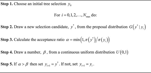The algorithm is outlined in Figure A1.

Figure A1. Metropolis algorithm.

References

- Baldwin VCJ, Feduccia DP, Haywood JD. 1989. Postthinning growth and yield of row-thinned and selectively thinned loblolly and slash pine plantations. Can J For Res. 19:247–256. doi: 10.1139/x89-035
- Bergh J, Linder S, Lundmark T, Elfving B. 1999. The effect of water and nutrient availability on the productivity of Norway spruce in northern and southern Sweden. For Ecol Manage. 119:51–62. doi: 10.1016/S0378-1127(98)00509-X
- Bredberg CJ. 1972. Type stands for the first thinning. Stockholm: Royal College of Forestry. Nr 52.
- Canham CD, LePage PT, Coates KD. 2004. A neighborhood analysis of canopy tree competition: effects of shading versus crowding. Can J For Res. 34:778–787. doi: 10.1139/x03-232
- Cao T, Hyytiäinen K, Tahvonen O, Valsta L. 2006. Effects of initial stand states on optimal thinning regime and rotation of Picea abies stands. Scand J For Res. 21:388–398. doi: 10.1080/02827580600951915
- Clark PJ, Evans FC. 1954. Distance to nearest neighbor as a measure of spatial relationships in populations. Ecology. 35:445–453. doi: 10.2307/1931034
- Contreras MA. 2010. Spatio-temporal optimization of tree removal to efficiently minimize crown fire potential [dissertation]. The University of Montana.
- Contreras MA, Chung W. 2013. Developing a computerized approach for optimizing individual tree removal to efficiently reduce crown fire potential. For Ecol Manage. 289:219–233. doi: 10.1016/j.foreco.2012.09.038
- Cronie O, Nystro K, Yu J. 2013. Spatiotemporal modeling of Swedish Scots pine stands. For Sci. 59:505–516.
- Edgren V, Nylinder P. 1949. Funktioner och tabeller för bestämning av avsmalning och formkvot under bark för tall och gran i norra och södra Sverige [Functions and tables for computing taper and form quotient inside bark for pine and spruce in northern and southern Sweden]. Stockholm: Statens skogsforskningsinstitut. Band 38 Nr 7. Swedish.
- Elfving B. 2010. Natural mortality in thinning and fertilisation experiments with pine and spruce in Sweden. For Ecol Manage. 260:353–360. doi: 10.1016/j.foreco.2010.04.025
- Eriksson M, Lindroos O. 2014. Productivity of harvesters and forwarders in CTL operations in northern Sweden based on large follow-up datasets. Int J For Eng. 25:179–200.
- Gilks WR, Richardson S, Spiegelhalter DJ. 1996. Markov chain Monte Carlo in practice. London: Chapman & Hall/CRC Press.
- Grimm V, Railsback S. 2005. Individual-based modeling and ecology. Princeton: Princeton University Press.
- Hyytiäinen K, Hari P, Kokkila T, Mäkelä A, Tahvonen O, Taipale J. 2004. Connecting a process-based forest growth model to stand-level economic optimization. Can J For Res. 34:2060–2073. doi: 10.1139/x04-056
- Hyytiäinen K, Tahvonen O. 2003. Maximum sustained yield, forest rent or Faustmann: does it really matter? Scand J For Res. 18:457–469. doi: 10.1080/02827580310013235
- Kot M. 2001. Elements of Mathematical Ecology. Igarss 2014.
- Leopold DJ, Parker GR, Ward JS. 1985. Tree spatial patterns in an old-growth forest in east-central Indiana. In: Dawson, JO and Majerus, KA, editors. Proceedings of the Fith Central Hardwood forest Conference; April 15-17; Urbana-Champaign (IL). p. 151–164.
- Liu J, Ashton PS. 1998. FORMOSAIC: an individual-based spatially explicit model for simulating forest dynamics in landscape mosaics. Ecol Modell. 106:177–200. doi: 10.1016/S0304-3800(97)00191-9
- Mäkinen H, Isomäki A. 2004. Thinning intensity and growth of scots pine stands in Finland. For Ecol Manage. 201:311–325. doi: 10.1016/j.foreco.2004.07.016
- Mäkinen H, Isomäki A, Hongisto T. 2006. Effect of half-systematic and systematic thinning on the increment of scots pine and Norway spruce in Finland. Forestry. 79:103–121. doi: 10.1093/forestry/cpi061
- Mielikäinen K, Valkonen S. 1991. Effect of thinning method on the yield of middle-aged stands in southern Finland. Folia For. 776, 22 p. Finnish with English summary.
- Nilsson U, Agestam E, Ekö PM, Elfving B, Fahlvik N, Johansson U, Karlsson K, Lundmark T, Wallentin C. 2010. Thinning of scots pine and Norway spruce monocultures in Sweden – effects of different thinning programmes on stand level gross- and net stem volume production. Stud For Suec. 219:1–46.
- Nurminen T, Korpunen H, Uusitalo J. 2006. Time consumption analysis of the mechanized cut-to-length harvesting system. Silva Fenn. 40:335–363. doi: 10.14214/sf.346
- Pacala SW, Canham CD, Saponara J, Silander Jr JA, Kobe RK, Ribbens E. 1996. Forest models defined by field measurements: estimation, error analysis and dynamics. Ecol Monogr. 66:1–43. doi: 10.2307/2963479
- Phillips PD, Van Gardingen PR. 2001. The SYMFOR framework for individual-based spatial ecological and silvicultural forest models. SYMFOR technical note series, 8.
- Pukkala T. 2015. Optimizing continuous cover management of boreal forest when timber prices and tree growth are stochastic. For Ecosyst. 2:1–13. doi: 10.1186/s40663-014-0025-0
- Pukkala T, Lähde E, Laiho O. 2013. Species interactions in the dynamics of even- and uneven-Aged Boreal Forests. J Sustain For. 32:371–403. doi: 10.1080/10549811.2013.770766
- Pukkala T, Miina J, Kurttila M, Kolstrom T. 1998. A spatial yield model for optimizing the thinning regime of mixed stands of Pinus sylvestris and Picea abies. Scand J For Res. 13:31–42. doi: 10.1080/02827589809382959
- Seidl R, Rammer W, Scheller RM, Spies TA. 2012. An individual-based process model to simulate landscape-scale forest ecosystem dynamics. An Ecol Modell. 231:87–100. doi: 10.1016/j.ecolmodel.2012.02.015
- Sinclair DF. 1985. On tests of spatial randomness using mean nearest neighbor distance. Ecology. 66:1084–1085. doi: 10.2307/1940568
- Solberg B, Haight RG. 1991. Analysis of optimal economic management regimes for Picea abies stands using a stage-structured optimal-control model. Scand J For Res. 6:559–572. doi: 10.1080/02827589109382692
- Valsta L. 1992a. An optimization model for Norway spruce management based on individual-tree growth models. Acta Forestalia Fennica.
- Valsta L. 1992b. A scenario approach to stochastic anticipatory optimization in stand management. For Sci. 38:430–447.
- Wallentin C. 2007. Thinning of Norway spruce [dissertation]. Alnarp: Swedish University of Agricultural Sciences.
- Zeide B. 2001. Thinning and growth: a full turnaround. J For. 99:20–25.