Using hybrid modelling to predict basal area and evaluate effects of climate change on growth of Norway spruce and Scots pine stands

ABSTRACT

When modelling forest growth, capturing the effects of climate change is needed for reliable long-term predictions and management choices. This remains a challenge because commonly used mensurational forest growth and yield models, relying on inventory data, cannot account for climate change effects. We developed hybrid physiological/mensurational basal area growth and yield models, which combine physiological response to climatic conditions and empirical relations. We included climate and site effects by replacing time with light sums of photosynthetically active radiation and modifying the latter with monthly soil water, vapour pressure deficit, temperature, and frost days. When parameterised with permanent sample plot data for Scots pine and Norway spruce across Sweden, the hybrid models could reproduce observations well, although with no increase in precision compared with time-based mensurational models. When considering different climate scenarios, a significant impact on productivity from climate change emerged. For example, a 2 °C warming enhanced Scots pine production by up to 14% in regions where temperatures were originally cooler and soil water deficit was low (i.e. northwest Sweden), but depressed it, up to 9%, elsewhere. Hence, climate-sensitive models that take local variations into account are necessary for accurate predictions and sustainable forest management.

KEYWORDS:

• photosynthetically active radiation
• forest modelling
• boreal forests
• growth and yield
• long-term prediction

Introduction

Growth and yield models are essential tools for sustainable management of forest resources. The commonly used mensurational models, which use inventory data to identify relationships based on correlations, can effectively predict forest development under the conditions used for their parameterisation. Nevertheless, they cannot reliably simulate the effects of growth conditions beyond the ranges covered by the parameterisation data (Weiskittel et al. 2011). This is a major limitation when considering the effects of climate change on forest productivity (Boisvenue and Running 2006; Martin-Benito and Pederson 2015), because of less accurate long-term projections and limited ability to make sustainable management decisions. Therefore, there is a need for models and prediction tools to take climate change into account.

One approach is the integration of some aspects of ecophysiology into forest growth and yield models, like the ability of forests to utilise incoming solar radiation to produce wood through photosynthesis (Monteith 1977; Mason et al. 2011). A way to take these physiological concepts into account without excessive complexity is to use a hybrid modelling approach. Hybrid models avoid key shortcomings of empirical mensurational models by combining them with process-based physiological models (Johnsen et al. 2001; Weiskittel et al. 2011). At the same time, hybrid models avoid the limitations of process-based models, which capture the underlying processes that make trees and forests grow, like light interception, carbon allocation, and water and nutrient cycles. Taking these underlying processes into account can lead to complex model systems that are difficult to use in practical forestry due to their parameter and computational requirements. The lack of understanding of some forest growth processes also hinders accurate predictions from purely physiological models (Taylor et al. 2009; Weiskittel et al. 2011).

Hybrid models can be divided into three categories. First, models using an external growth modifier, i.e. the growth predicted by the mensurational model is adjusted by a modifier derived from mechanistic models (Henning and Burk 2004). Second, physiologically derived covariate models, where parts of a mensurational model are replaced by or complemented with covariates created using physiological process models (Baldwin et al. 2001; Mason et al. 2007). Third, allometric models, which are closer to process-based modelling as they are based on physiological sub-models but rely on statistical patterns to explain the relationship between stem dimensions and biomass (Landsberg and Waring 1997).

The predictive performance of hybrid models are often better than pure mensurational models, but varies greatly depending on the model resolution, species and type of hybridisation (Weiskittel et al. 2011). Stand-level models have significantly improved predictions (Battaglia et al. 1999; Snowdon 2001; Dzierzon and Mason 2006), while the performance gains from hybridising tree-level models are less clear (Henning and Burk 2004; Weiskittel et al. 2010). At the stand level, the performance gain depends on the output variable, with predictions of basal area improving more than height (Snowdon 2001; Dzierzon and Mason 2006). However, the extent of model improvement declines over longer prediction periods (Snowdon 2001). Beyond improved predictive performance, a major gain from the hybrid modelling approach is the possibility to introduce climate sensitivity into growth and yield models (Subramanian et al. 2019; Rachid-Casnati et al. 2020). The hybrid models should flexibly incorporate changing growing conditions to capture climate change effects on forest production. This added flexibility allows for better precision and long-term projections and the opportunity to investigate climate change impacts on forest productivity.

Climate change is expected to result in further temperature increases and, in many regions, changes in precipitation patterns (IPCC 2021). In boreal regions of northern Europe, temperature is predicted to increase considerably, and more so at higher latitudes (Cattiaux et al. 2013; Jacob et al. 2014). Average annual temperatures are expected to increase by 1 °C at latitude 55° N and 2 °C at 68° N in Europe by the end of the twenty-first century for the RCP2.6 scenario, and of 4 and 7 °C respectively for the RCP8.5 scenario (Jacob et al. 2014; SMHI 2020a). Precipitation projections are less certain, but winter could become wetter and summers drier or remain unchanged, with considerable local variation (Eklund et al. 2015; Ruosteenoja et al. 2018; SMHI 2020a).

These changes in climate will affect European forest biomass production, which is centred in northern Europe. A significant part of that biomass consists of conifer forests in Sweden (Rytter et al. 2015). In Sweden, 58% (23.6 million ha) of the land area is covered by productive forest. The dominant tree species are Scots pine (Pinus sylvestris L.) and Norway spruce (Picea abies (L.) Karst.), which together represent 80% of Sweden’s standing volume (SLU 2021). These forests deliver important ecosystem services such as wood production and carbon sequestration, helping reduce European carbon footprint (Rytter et al. 2016; Felton et al. 2020). This makes forest productivity a crucial issue and highlights the need for models that can predict climate change effects on forest growth in an uncertain future.

Warmer temperatures will likely accelerate forest growth since temperature is often the most limiting factor in this region (Bergh et al. 1999; Allen et al. 2010). Some of these expected positive effects have already been seen (Mensah et al. 2021), with faster height growth under increased temperatures. However, higher temperatures combined with unchanged or reduced precipitation could lead to drought stress becoming more common during the growing season (Ruosteenoja et al. 2018). Climate change could then reduce forest productivity in locations and years where the available water is depleted via faster evapotranspiration (Belyazid and Zanchi 2019; Ruiz-Pérez and Vico 2020). An example of this was the hot and dry summer of 2018 that reduced forest productivity in central and northern Europe (Peters et al. 2020). The net effect of climate change on northern European forests is unclear.

Models able to capture climate impacts on productivity can help support management decisions, like choice of species and timing of silvicultural treatments. However, there is a lack of climate-sensitive hybrid models applicable to boreal forests in northern Europe. One option is the 3PG model (Landsberg and Waring 1997) but it is still relatively complex (Landsberg et al. 2005) and so far only parameterised on a regional scale (Subramanian et al. 2019). Most climate-sensitive hybrid models with physiologically derived covariates or external growth modifiers are developed for plantation forestry of fast-growing species (Pinjuv et al. 2006; Mason et al. 2011; Rachid-Casnati et al. 2020). No such models exist for conifer forests in northern Europe that can be applied to a wide variety of sites.

In this study, building on the potentially usable light sum equation (PULSE) hybrid approach (Mason et al. 2007) we developed and compared several hybrid physiological/mensurational basal area yield models, to capture the effects of potentially key environmental conditions (vapour pressure deficit, soil water availability, temperature, and occurrence of frost days). The models were applied to Scots pine and Norway spruce in Sweden, and their prediction capacity was compared with traditional mensurational models. The overarching goals were i) to develop hybrid models with an improved predictive ability, compared with traditional mensurational models; and ii) test the hypothesis that plausible future climates scenarios with higher temperatures and increased precipitation would yield higher basal area growth compared with current climate.

Materials and methods

Modelling data

Data from the Swedish National Forest Inventory (NFI), Swedish long-term forest experiments, and Swedish Meteorological and Hydrological Institute (SMHI) were used for model fitting and validation. The Swedish NFI covers the entire country with temporary and permanent sample plots to monitor and provide data on all Swedish forests. The NFI is designed as a systematic sample grid with a random grid position, where the plots are clustered into square and rectangular clusters (Fridman et al. 2014). Here we took advantage of the Swedish NFI data from permanent plot inventories, with repeated measurements between 1983 and 2017. Every permanent plot was measured once every five years, except between 1993–2002, when the remeasurement period was 5–10 years. All trees with a diameter at breast height (DBH, at 1.3 m) of 10 cm or larger were measured in a 10 m radius plot. Trees between 4 and 10 cm DBH were measured in a subset of the plot. The size of this subset changed over time. From 2003 onward, the small plot was a 3.5 m radius circle, but between 1993 and 2002, the small plot was a quarter circle with a 5 m radius. Beyond measuring the living trees, all trees that had been cut or died since the previous census and damaged trees were recorded starting in 1988, including the cause of death or damage. Apart from tree measurements, other general stand and site properties were recorded, such as ground vegetation, soil texture, and previous management history (Fridman et al. 2014).

The NFI data used for model fitting and validation were limited to plots inventoried from 1993 to 2017. However, data from permanent plots from before 1993 were used in data management to prepare consistent age and thinning variables. All possible periods between 1993–2017 were used in model fitting to make the models as robust as possible (Lee 1998), resulting in a varied measurement interval from 5 to 20 years. The steps taken to manage the NFI and long-term experiment data before model implementation are detailed in Appendix A.

The Swedish long-term forest experiment data come from even-aged monocultures of Norway spruce and Scots pine from Scania county in the south to Norrbotten county in the north. The experiments were mainly focused on fertilisation, regeneration, spacing, and thinning in stands established through planting, seeding, or natural regeneration (Elfving and Kiviste 1997; Nilsson et al. 2010). The mean plot area was 0.06 ha (range 0.02–0.2 ha). Measurements were made between 1960 and 2017, and the measurement interval ranged from 1 to 36 years (mean = 8 years).

From the around 15000 permanent NFI plots and 7000 long-term experiment plots available, we selected 1922 plots for Scots pine for modelling and validation, of which 411 were long-term experiment plots and 1511 NFI plots, covers the entire country. For Norway spruce, 836 plots were used for modelling and validation, of which 219 were long-term experiment plots and 617 NFI plots. These plots corresponded to 7798 growth periods (2219 from experimental plots and 5579 from NFI plots) for Scots pine and 4623 growth periods (1658 from experimental plots and 2965 from NFI plots) for Norway spruce. The plot selection was based on plot properties like species composition, tree height and previous management. A more detailed description of the plot selection can be found in Appendix A.

We obtained monthly accumulated estimates of photosynthetically active radiation (PAR), global radiation on a horizontal surface (GHI), precipitation, and maximum, minimum, and mean temperatures from 1958 to 2017 from SMHI. The data was provided in 11*11 km raster files based on UERRA reanalyses (SMHI 2020b), where each permanent plot was linked to the closest pixel. Monthly temperatures were adjusted for elevation differences between measured plots the temperature raster points.

Model description

We built upon the potentially usable light sum equation (PULSE) hybrid approach (Mason et al. 2007) to hybridise mensurational models. The PULSE approach develops a hybrid model with physiologically derived covariates, where stand ages are substituted with potentially usable light sum (PULS) (see below) in a compatible growth and yield equation. To increase model sensitivity to site and climate, the monthly PAR was modified based on the 3PG-model (Landsberg and Waring 1997) and then summed up to PULS. The PULSE approach was successfully implemented for plantations of Douglas-fir (Pseudotsuga menzeisii (Mirb.) Franco) in the USA (Mason et al. 2007), radiata pine (Pinus radiata D. Don.) in New Zealand (Mason et al. 2011), and Eucalyptus grandis and Pinus taeda in Uruguay (Rachid-Casnati et al. 2020). In these applications, with the hybrid models had performance on par or higher compared with mensurational time-based models.

Mensurational model

As starting point for the PULSE hybrid model, we developed one mensurational time-based model for Scots pine and one for Norway spruce, using the Schumacher (1939) equation augmented by initial plot stem number before thinning (Equation 1): (1) $G_2=e^{\log \left(G_1\right){\left({\displaystyle \frac{t_1}{t_2}}\right)}^{bS{T}^c}+a\left(1-{\left({\displaystyle \frac{t_1}{t_2}}\right)}^{bS{T}^c}\right)}$(1) where G₁ and G₂ are the total basal area (m² ha⁻¹) at the beginning and end of the measurement period, t₁ and t₂ are stand ages (years) at the beginning and end of the period, ST is initial stem number (stems ha⁻¹) before thinning, and a, b and c are parameters to be estimated. The Schumacher (1939) equation complies with the properties of a compatible growth and yield model defined in Clutter (1963). The mensurational model was fitted to the inventory data using the nonlinear least squares function (nls) in the R (version 3.6.1) statistical computing platform (R Core Team 2016).

Hybridisation of the mensurational model and determination of the potentially useable light sum

To hybridise the mensurational model, they were refitted with the same plot data and compatible growth and yield equation (Schumacher 1939). However, the time variables were replaced with PULS (Equation 2). PULS accumulated from stand establishment to t₁ (PULS₁), and PULS accumulated from establishment to t₂ (PULS₂) replaced the stand age variables t₁ and t₂. For example, if t₁ was 50 years, it was replaced by PULS accumulated for those 50 years. The hybrid model form is thus: (2) $G_2=e^{log\left(G_1\right){\left({\displaystyle \frac{PUL{S}_1}{PUL{S}_2}}\right)}^{bS{T}^c}+a\left(1-{\left({\displaystyle \frac{PUL{S}_1}{PUL{S}_2}}\right)}^{bS{T}^c}\right)}$(2) PULS in the hybrid model was calculated from monthly total PAR values in MJ m⁻². To better reflect potential photosynthesis, the monthly PAR was adjusted to climate and site properties by multiplying the radiation by a set of modifiers before summing it between the times of establishment and inventory (PULS_t); (3) $\mathrm{P}\mathrm{U}\mathrm{L}{\mathrm{S}}_t=\sum _{\mathrm{i}=1}^{\mathrm{t}}{\mathrm{R}}_{\mathrm{i}}\mathrm{m}\mathrm{i}\mathrm{n}\left(f_T,f_F\right)\mathrm{m}\mathrm{i}\mathrm{n}\left(f_W,f_D\right)$(3) where R_i is the total PAR for month i (MJ m⁻²), f_T is the modifier for temperature, f_F is the frost modifier, f_W is the soil water modifier, and f_D is the vapour pressure deficit (VPD) modifier, each in month t (Figure 1). All the modifiers (presented below) are non-dimensional and ranging between 0 and 1. In Equation (3), the minimum value of f_W or f_D was used because both modifiers affect tree water availability and use. Similarly, the minimum of f_T and f_F was used since both affect photosynthetic response to temperature.

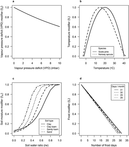
Figure 1. Functions for calculating modifiers used to adjust incoming radiation (PAR) values according to the following monthly variables. a) vapour pressure deficit (VPD). b) mean monthly temperature (°C) by species. c) soil water ratio (soil water balance (mm) (S) divided by the potentially available soil water (mm) (Φ) (see equation 10). d) number of frost days in a month.

PULS and climatic condition modifiers were calculated based on climate data from SMHI from 1958-2017. If the time of planting was before 1958, summed PAR from 1958 to 1968 was re-proportioned to account for the missing years and give an estimated PULS for the entire growth period.

Climatic condition modifiers

The modifier functions (Figure 1) were based on the 3PG model (Landsberg and Waring 1997), but the underlying water balance calculations were modified to fit available data and regional conditions better.

The VPD modifier is built around the relationship between monthly mean daytime vapour pressure deficit (VPD) and leaf stomatal conductance, where increasing VPD causes the leaf to close its stomata to reduce water losses (Grossiord et al. 2020). Stomatal closure also reduces photosynthesis and hence fixed carbon. The modifier declines exponentially with increasing VPD as: (4) $f_D=e^{-k_{g}VPD}$(4) where k_g (0.05 mbar) is a constant based on the relationship between VPD (mbar) and stomatal conductance relation (Sand 2004). VPD (mbar) is calculated as follows (Mason et al. 2007): (5) $VPD={\displaystyle \frac{D{T}_{max}-D{T}_{min}}{2}}$(5) where DT_max and DT_min are the saturated vapour pressure when the temperature is equal to the monthly maximum (T_a-max) and minimum (T_a-min) temperature respectively. These are calculated based on the temperature as: (6) $D{T}_i=0.61078e^{{\displaystyle \frac{17.269T_i}{T_i+237.3}}}$(6) where T_i is either the monthly maximum or minimum temperature (°C) (Allen et al. 1998).

The temperature modifier captures the increase in net photosynthesis with temperature until the optimum temperature; and its decline beyond that (Bergh et al. 1998; Kolari et al. 2007; Way and Yamori 2014). There is also a minimum temperature, which indicates the lowest temperature for net photosynthesis. The minimum was used to indicate when growth stopped for winter and started again for spring. The temperature modifier is computed as follows: (7) $f_T=\{\begin{array}{cc}\left({\displaystyle \frac{T_{ec}-T_{min}}{T_{opt}-T_{min}}}\right){({\displaystyle \frac{T_{max}-T_{ec}}{T_{max}-T_{opt}})}}^{{\displaystyle \frac{\left(T_{max}-T_{opt}\right)}{\left(T_{opt}-T_{min}\right)}}}& T_{min}<T_{ec}<T_{max}\\ 0& T_{max}\le T_{ec}\mathrm{o}\mathrm{r}{T}_{ec}\le T_{min}\end{array}$(7) where T_max, T_min and T_opt (°C) were the species-dependent maximum, minimum, and optimum temperatures for net photosynthesis. T_ec was the monthly mean daytime temperature. We used daytime mean temperature because it gives better precision than using daily means (Mason et al. 2011). T_ec was calculated assuming that diurnal temperature change is sinusoidal with minimum at 3 AM and maximum at 3 PM (Mason et al. 2011) using monthly maximum (T_a-max) and minimum (T_a-min) temperatures as extremes: (8) $T_{ec}=T_{a\mathrm{\_}max}0.7575+T_{a\mathrm{\_}min}0.2425$(8)

The soil water modifier captures the decrease in growth due to water stress by lowering PULS. The soil water modifier is: (9) $f_w={\displaystyle \frac{1}{1+{\left({\displaystyle \frac{1-r_w}{c_{\theta }}}\right)}^{n_{\theta }}}}$(9) where c_θ and n_θ are constants depending on soil type, and r_w is the ratio between plant-available soil water at the end of the month (S) and the maximum possible plant-available soil water (Φ), both referred to the rooting zone, i.e. (10) $r_w={\displaystyle \frac{\mathrm{S}}{\mathrm{\Phi }}}$(10) Φ was estimated using soil-specific porosity (Clapp and Hornberger 1978) together with the proportion of soil water that is plant-available (Andersson and Wiklert 1972; Dunne and Willmott 1996) and the mean rooting depth of boreal coniferous forests (Jackson et al. 1996). The maximum plant-available water in the rooting zone (Φ) was set to 104 mm soil for gravel and sand, 148 mm for loamy sand, 192 mm for sandy loam, 240 mm for loam, 296 mm for silt, 208 mm for clay, and 350 mm for peat. Some of the long-term experiment plots lacked soil texture information and were assumed to have sandy loam texture, the most common texture in the Swedish NFI data.

S was estimated using a monthly soil water balance based on a modified T-model (Alley 1984). Depending on whether potential evapotranspiration (E₀) was higher or lower than monthly precipitation (P) and temperature, the soil water content at the end of the month, S_t, was determined as: (11) $S_t=\{\begin{array}{cc}min\left(\left(P-E_0\right)+S_{t-1},\mathrm{\Phi }\right)& P\ge E_0\mathrm{a}\mathrm{n}\mathrm{d}{T}_a\ge 5{}^{\circ }\mathrm{C}\\ S_{\mathrm{t}-1}\exp \left(-{\displaystyle \frac{E_0-P}{\mathrm{\Phi }}}\right)& P<E_0\mathrm{a}\mathrm{n}\mathrm{d}{T}_a\ge 5{}^{\circ }\mathrm{C}\\ \mathrm{\Phi }& T_a<5{}^{\circ }\mathrm{C}\end{array}$(11) where S_t-1 is the soil water content at the end of the previous month. The soil was thus assumed to always be saturated (S_t= Φ) if T_a < 5 °C, regardless of precipitation inputs and evapotranspiration losses, to account for water storage in ice and snow during winter.

Potential evapotranspiration was estimated with the Priestley and Taylor (1971) formula as: (12) $E_0=\alpha {\displaystyle \frac{\mathrm{\Delta }}{\mathrm{\Delta }+\gamma }{\mathrm{r}}_n}$(12) where α is a constant (set at 1.26), Δ is the slope of the saturated vapour pressure curve, γ is the psychrometric constant, and r_n is net radiation.

The slope of the saturated vapour pressure curve was calculated as (Allen et al. 1998): (13) $\mathrm{\Delta }={\displaystyle \frac{4098\left(0.6108\exp \left({\displaystyle \frac{17.27\mathrm{T}\mathrm{a}}{\mathrm{T}\mathrm{a}+237.3}}\right)\right)}{{\left(\mathrm{T}\mathrm{a}+237.3\right)}^2}}$(13) Net radiation was estimated from the linear relationship between net radiation and total shortwave radiation (GHI) (Wm⁻²). The intercept (q_a) is −90 Wm⁻², and the slope (q_b) is 0.8 (Sand 2004). (14) $r_n=\left(q_a+q_{b}GHI\right)$(14) The psychrometric constant (γ) was determined as (Allen et al. 1998): (15) $\gamma =0.665\ast {10}^{-3}{P}_a$(15) where P_a is the atmospheric pressure (kPa) calculated using plot-specific elevation (alt; m above sea level): (16) $P_a=101.3{\left({\displaystyle \frac{293-0.0065alt}{293}}\right)}^{5.26}$(16) Finally, the frost modifier assumed that monthly photosynthesis is reduced proportionally to the number of days with a minimum temperature < 0 °C during the month (Landsberg and Waring 1997). The frost modifier was calculated as: (17) ${\mathrm{f}}_{\mathrm{F}}=1-{\displaystyle \frac{\mathrm{N}\mathrm{u}\mathrm{m}\mathrm{b}\mathrm{e}\mathrm{r}\mathrm{o}\mathrm{f}\mathrm{f}\mathrm{r}\mathrm{o}\mathrm{s}\mathrm{t}\mathrm{d}\mathrm{a}\mathrm{y}\mathrm{s}\mathrm{p}\mathrm{e}\mathrm{r}\mathrm{m}\mathrm{o}\mathrm{n}\mathrm{t}\mathrm{h}}{\mathrm{N}\mathrm{u}\mathrm{m}\mathrm{b}\mathrm{e}\mathrm{r}\mathrm{o}\mathrm{f}\mathrm{d}\mathrm{a}\mathrm{y}\mathrm{s}\mathrm{p}\mathrm{e}\mathrm{r}\mathrm{m}\mathrm{o}\mathrm{n}\mathrm{t}\mathrm{h}}}$(17)

Model fitting and evaluation

Model fitting was based on two-thirds of the NFI and long-term experiment plots, with the remaining third used for validation. The modelling procedure was used for fitting both the time-based (Equation 1) and hybrid (Equation 2) models. When fitting the hybrid models, models containing only one modifier (i.e. setting other f values in Equation 3–1) were first considered to see each modifier’s effect independently. After that, models containing all modifiers were considered.

The time-based and hybrid models were compared by applying them to the validation dataset and analysing residuals. Precision, bias, and normality of residuals were assessed when comparing models by examining root mean square error (RMSE), means and plots of residuals, and residuals frequency distributions. Parameter significance was checked by fitting the models to a random sub-sample containing one interval per plot to reduce autocorrelation effects.

All model fitting, data management and statistical analyses were done in R (version 3.6.1) (R Core Team 2016).

Sensitivity analysis on climate change

A sensitivity analysis was performed on the hybrid models to test the impact of changing climatic conditions according to scenarios of temperature and precipitation increase. Observed conditions between 1993 and 2013 were altered to determine the growth over a hypothetical 20-year period under changed climate. Monthly temperatures were increased by 2 or 4 °C, and monthly precipitation was increased by either 10 or 20%. To account for the change in frost days due to increasing temperatures, the number of frost days was reduced by 25% if the temperature increased by 2 °C and 50% if the temperature increased by 4 °C (Meehl et al. 2004). These changes were in line with the predicted average changes to summer (June, July, August) climate for the end of the twenty-first century in northern Europe for the RPC2.6 and RPC8.5 climate scenarios respectively (SMHI 2020a).

140 NFI plots from all over Sweden were randomly selected for the climate analysis from the third of the plots used for validation. All plots were assigned a starting basal area of 20 m² ha⁻¹, an age of 35 years and an initial plot stem number before thinning of 1500 stems ha⁻¹ for Scots pine and 2000 stems ha⁻¹ for Norway spruce, with unchanged climate data. The species-specific hybrid models containing all modifiers (Hybrid-TFDW) simulated basal area development for 20 years using observed and altered climate data. Predicted basal area values were compared to evaluate the effects of changing climatic conditions on the hybrid model output. The baseline for this comparison was the predicted basal area using observed climate data. Predicted basal areas for the scenarios with altered climate data were then compared against this baseline. The comparison was presented as the relative change (%) in basal area for each climate scenario and species-specific model. Differences between scenarios and between species-specific hybrid models were evaluated using Tukey's (HSD) test following analysis of variance (p < 0.05) with the following models (Equation 18 and 19). Equation 18 was used separately for each species to test differences between scenarios: (18) $Y=SC+e$(18) where Y is the relative difference (%) in basal area compared to the baseline, SC is the climate scenario, and e is the error. Equation 19 was used to test the difference in response between the species-specific hybrid models, separately for each scenario, where TS is tree species (either Scots pine or Norway spruce): (19) $Y=TS+e$(19)

Results

Model performance

Both the time-based and hybrid models with single and combined modifiers showed a good and relatively unbiased fit against the model data with similar patterns for Scots pine (Figures 2 and A.1). Similar results were obtained for Norway spruce (Figures 3 and A.2). When comparing the residuals for the different tested models, there were minor differences, and the hybrid models did not have a better fit (i.e. smaller RMSE) than the time-based models (Table 2).

Figure 2. Residuals of the fitted mensurational time-based model (a) and the hybrid model (Hybrid-TFDW) (b) for Scots pine. Residuals from the validation of the mensurational time-based model (c) and the hybrid model (Hybrid-TFDW) (d). The thick lines show the trend in the residuals.

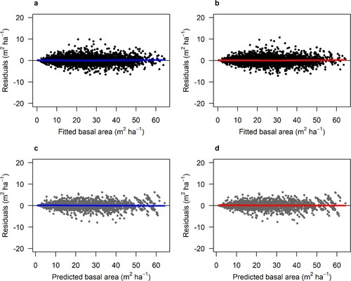
Figure 3. Residuals of the fitted mensurational time-based model (a) and the hybrid model (Hybrid-TFDW) (b) for Norway spruce. Residuals from the validation of the mensurational time-based model (c) and the hybrid model (Hybrid-TFDW) (d). The thick lines show the trend in the residuals.

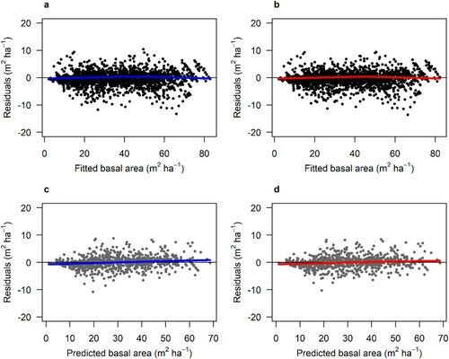
Table 1. Variables and parameters used in the climate modifier calculations.

Parameter or variable	Symbol	Unit	Value	Reference
Monthly mean daytime vapour pressure deficit	VPD	mbar
Canopy response to VPD	kg	mbar	0.05	(Sand 2004)
Monthly average of the daily temperature	Ta	°C
Monthly average of the daily minimum temperature	Ta-min	°C
Monthly average of the daily maximum temperature	Ta-max	°C
Monthly average daytime temperature	Tec	°C
Species-specific maximum, minimum, and optimum temperatures for photosynthesis:
Pinus sylvestris	Tmax, Tmin and Topt	°C	40, −2, 20	(Kolari et al. 2007)
Picea abies	Tmax, Tmin and Topt	°C	42, −3, 15	(Bergh et al. 1998)
Soil water modifier coefficient for clay, clay loam, sandy loam, and sandy soils	cθ		0.4, 0.5, 0.6, 0.7	(Landsberg and Waring 1997)
Soil water modifier exponent for clay, clay loam, sandy loam, and sandy soils	nθ		3, 5, 7, 9	(Landsberg and Waring 1997)
Atmospheric pressure	Pa	kPa
Slope of the saturation vapour pressure curve	Δ	kPa°C^−1
Psychrometric parameter	γ	kPa°C^−1
Net radiation	Rn	kWh m^−2
Total shortwave radiation	GHI	kWh m^−2
Intercept and slope of the relationship between Rn and GHI	qa, qb	Wm^−2	−90, 0.8	(Landsberg and Sands 2011)
Photosynthetically active radiation	PAR	MJm^−2
Monthly precipitation	P	mm
Interception	I	mm
Potential evapotranspiration	E0	mm
Actual evapotranspiration	E	mm
Plant available soil water balance in the root zone at the end of the month	S	mm
Soil water balance previous month	St-1	mm
Potentially plant-available soil water in the root zone	Φ	mm
Soil water ratio between S and Φ	rw

Table 2. Estimated parameters for the fitted basal area models and their standard errors (SE) and model fit and validation RMSE (m² ha⁻¹). Time-based (Equation 1) = mensurational model using time as driving variable. Hybrid (Equation 2) = unmodified PULS, Hybrid-D = modified by VPD, Hybrid-W = modified by soil water, Hybrid-T= modified by temperature, Hybrid-F= modified by frost, and Hybrid-TFDW= all four modifiers included. All estimated parameters were significant (p-value < 0.05).

Species	Model		Parameter			RMSE (m^2 ha^−1)
			a	b	c	Model fitting	Validation
Scots pine	Time-Based	Estimate	4.822	0.151	0.224	1.404	1.471
		SE	0.017	0.006	0.006
	Hybrid	Estimate	4.816	0.156	0.224	1.393	1.470
		SE	0.017	0.007	0.006
	Hybrid-D	Estimate	4.816	0.151	0.228	1.398	1.473
		SE	0.017	0.007	0.006
	Hybrid-T	Estimate	4.806	0.139	0.238	1.394	1.475
		SE	0.016	0.006	0.006
	Hybrid-W	Estimate	4.760	0.108	0.276	1.396	1.481
		SE	0.016	0.005	0.007
	Hybrid-F	Estimate	4.806	0.139	0.238	1.394	1.475
		SE	0.016	0.006	0.006
	Hybrid-TFDW	Estimate	4.728	0.076	0.324	1.396	1.485
		SE	0.016	0.006	0.007
Norway spruce	Time-Based	Estimate	5.113	0.328	0.119	2.507	2.279
		SE	0.018	0.022	0.009
	Hybrid	Estimate	5.089	0.303	0.137	2.472	2.242
		SE	0.017	0.020	0.009
	Hybrid-D	Estimate	5.082	0.281	0.148	2.465	2.238
		SE	0.017	0.018	0.009
	Hybrid-T	Estimate	5.098	0.287	0.143	2.483	2.252
		SE	0.018	0.019	0.009
	Hybrid-W	Estimate	5.092	0.195	0.192	2.476	2.194
		SE	0.018	0.013	0.009
	Hybrid-F	Estimate	5.097	0.259	0.156	2.476	2.262
		SE	0.017	0.017	0.009
	Hybrid-TFDW	Estimate	5.082	0.144	0.231	2.485	2.267
			0.018	0.010	0.009

The hybrid models showed minor differences in RMSE between predicted and measured basal area compared with the time-based mensurational models for both species during validation (Table 2). Both the hybrid and mensurational models showed good and unbiased predictions during validation with similar residual patterns for Scots pine (Figures 2 and A.3) and Norway spruce (Figures 3 and A.4).

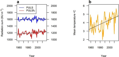
The unmodified PULS (blue line in Figure 4a) showed no significant trend over the 60 years, and anomalies with respect to the mean were small. When the radiation was modified by the temperature modifier (PULSf_T; red line in Figure 4a) it showed an increasing trend due to temperature increases during the period and sensitivity to especially warm and cold years. Both PULSf_T and mean annual temperature (Figure 4b) had a significant (p-value < 0.05) positive trend during the measurement period.

Figure 4. 140 randomly selected NFI plots, a) yearly radiation sum (MJ m⁻²) over the measurement period for unmodified PULS (MJ m⁻²; blue line), and PULS modified by temperature (PULSf_T; red line). b) yearly mean temperature (°C) at the same sites. The black lines show linear trends.

Climate sensitivity

Growth limitations

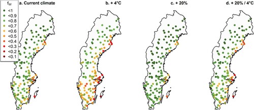
Under the current climatic conditions, soil water was a substantial limiting factor for growth (i.e. f_W was < 0.6), mostly in southern and eastern Sweden (Figure 5a), between June and September (Figure A.5). Outside those months, water was not limiting growth (f_W ≈ 1). Increased precipitation reduced the limitation imposed by soil water availability, with f_W increasing on average by 0.1 (i.e. 13%) in July when precipitation increased by 20% (Figure 5c). Increased temperature led to increased soil water limitation with f_W decreasing by 0.14 (18%) on average in July when temperatures increased by 4 °C (Figure 5b). When temperature and precipitation increased simultaneously, water availability was similar to current climate with no change to the average f_W values (Figure 5d). For VPD, there were limitations (f_D between 0.8 and 0.9) during April-September, with lower f_D values associated with monthly average temperatures over 20 °C (Figure A.6). Increased temperatures resulted in more limitation from VPD with an average decrease in f_D by 2% when temperatures increased by 4 °C, with similar geographical patterns.

Figure 5. Average effect for July of temperature and precipitation changes on the soil water modifier (f_W) during a 20-year simulation with altered input climate data. The dots represent randomly selected permanent sample plots from the Swedish NFI. The panels show scenarios of: (a) current climate, (b) temperature increased by 4 °C, (c) precipitation increased by 20%, and (d) precipitation increased by 20% and temperature increased by 4 °C.

Under current climate, temperature limitations were low during the summer months (June, July, and August), when the average monthly temperatures were around 15–20 °C, except for plots in the far northwest (f_T ≈ 0.9) where temperatures were lower (around 10–15 °C) (Figure A.7). Periods outside the summer had lower f_T values (f_T < 0.9), with f_T ≈ 0 in December, January, and February. As expected, temperature limitations increased with latitude (Figure A.7). The frost modifier patterns were similar, with no limitations (f_F ≈ 1) in the summer and increased limitations closer to winter (f_F < 0.1) (Figure A.8). Increased temperatures resulted in less frost and temperature limitation with the same geographical patterns. Increased temperatures by 4 °C resulted in an increase of f_F by 0.24 (47%) and f_T by 0.15 (28%) on average over the year.

Growth response

On average, all climate change scenarios resulted in a significantly (p-value < 0.05) increased basal area, except under the +2 °C warming scenario at current precipitation, where the result of the Norway spruce model was not significantly different from the current climate. The different scenarios yielded a considerable variation in response, especially when temperatures increased by 4°C (Figure 6). This variation in response depended on location (Figures 7 and 8), with increased temperatures leading to reduced growth in south-eastern Sweden and increased growth in the northwest. An increase in precipitation with unaltered temperature had the greatest positive effect on basal area development in the southern and eastern regions.

Figure 6. Relative change of basal area (%) after a 20-year simulation with altered input climate data compared with current climate. The different scenarios tested were increased monthly precipitation by either 10% or 20%, increased monthly temperatures by either 2 °C or 4 °C, and all four combinations of increased temperature and precipitation. All scenarios, except for the 2 °C warming scenario at current precipitation for Norway spruce, were significantly different (p-value < 0.05) from the unaltered climate scenario.

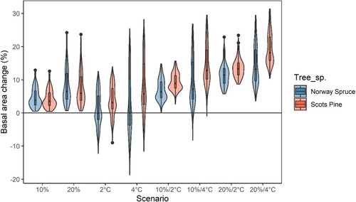
Figure 7. Relative change in basal area change (%) after a 20-year simulation with altered input climate data compared with current climate using the hybrid Scots pine model containing all modifiers (Hybrid-TFDW). The dots represent 140 randomly selected permanent sample plots from the Swedish NFI. Scenarios: (a) = increased temperature increased by 2 °C, (b) = increased precipitation increased by 10%, and (c) = increased precipitation increased by 10% and increased temperature increased by 2 °C.

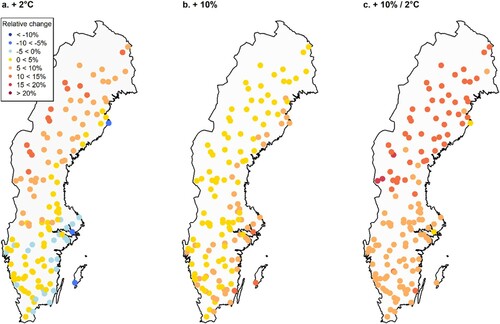
Figure 8. Relative change in basal area change (%) after a 20-year simulation with altered input climate data compared with current climate using the hybrid Norway spruce model containing all modifiers (Hybrid-TFDW). The dots represent 140 randomly selected permanent sample plots from the Swedish NFI. Scenarios: (a) = increased temperature increased by 2 °C, (b) = increased precipitation increased by 10%, and (c) = increased precipitation increased by 10% and increased temperature increased by 2 °C.

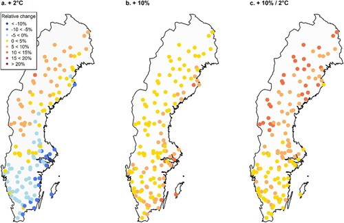
When combining the effects of increased temperature and precipitation, the positive effect on basal area was highest in the north. The geographical patterns were similar for the different temperature and precipitation scenarios and both species-specific models (Figure 7 and 8). For Norway spruce, there was a larger negative effect of increased temperatures in southern and eastern regions. There were also less positive effects of combined temperature and precipitation increases compared with Scots pine.

The difference in scenario response between the hybrid models for Norway spruce and Scots pine was significant (p-value < 0.05) for all scenarios except for the two scenarios where precipitation increased by 10 and 20%.

Discussion

Improvements in model performance by hybridisation

The hybrid models with climatic condition modifiers can easily take into account site and climatic conditions, including changes expected in the future. Long-term trends due to a changing climate can be accounted for, as seen in Figure 4, where the trend of increased temperature between 1958 and 2017 was captured in the modified PULS variable. If just time had been used, the model could not have included the effects of the increasing temperature and changed growth conditions as the hybrid model could with the temperature modifier. The same ability to capture changes in growing conditions could be seen when looking at the change in growth limitations (Figure 5). The soil water modifier (f_W) illustrates the ecophysiological response to a changing climate. Using this and other modifiers allows accounting for climatic conditions during growth predictions and provide opportunities to evaluate what factors limit growth the most. As seen in Figure 5a, even under current climate, soil water is a limiting factor for growth in parts of southern and eastern Sweden. This effect of water deficit on productivity is in line with previous findings and satellite data, where low precipitation and water availability decreased production and irrigation had positive effects on productivity in southern Sweden but not in the north (Bergh et al. 1999; Bergh et al. 2005; Ruiz-Pérez and Vico 2020). That limitation is either reduced or increased depending on climate scenario.

Against our expectations, there were only minor differences in precision between the time-based models and the hybrid models when compared against the validation data set (Table 2), even in the case on no climatic modifiers. Compared with other studies using the PULSE approach, there was a lack of improvement, pointing to the ability of even simple models to capture the key dynamics via their empirical parameters. A reason for this lack of significant improvement in precision could be the long rotations and slow growth of Scandinavian boreal forests, the main difference with respect to previous applications of the PULSE approach with climatic modifiers. Shorter rotations (10-30 yrs) and faster growth, like those of eucalyptus in Uruguay (Rachid-Casnati et al. 2020) and radiata pine in New Zealand (Mason et al. 2011), makes the results more sensitive to weather fluctuations during and between years. For example, if one year in a 10-year rotation was characterised by detrimental growing conditions, this single year would affects 10% of the rotation. This effect is larger, compared with e.g. a 70-year rotation, where a single unfavourable year would only affect 1.4% of the rotation. Short-term variation has a smaller effect with longer periods since it evens out in the long run (Snowdon 2001).

The climatic modifiers during the growing season were close to one in most parts of Sweden, showing that, under the current climate, the growth conditions captured by these models did not substantially limit growth. The only exception was the soil water modifier in south-eastern Sweden, where summer water deficit limited forest growth also under the current climate. The low limitation on growth from these factors could partly explain the lack of improvement of the hybrid models compared to other modelling approaches.

The lack of improvement could also result from how PULS was calculated. As described in the materials and methods, age is not an error-free variable in the Swedish NFI (Elfving 2010; Fahlvik et al. 2014). Since accumulated radiation is based on the estimated age, errors in the NFI age variable affect the modified PULS.

Relevance and uncertainties in the climate modifiers

Climatic conditions impacted basal area growth through the climate modifiers, reducing the incoming usable radiation. These modifiers require several input variables, which are not always directly measurable. Furthermore, to be simple enough for inclusion in a hybrid model, the modifiers cannot fully represent the complex plant physiological mechanisms and their responses to growing conditions. For example, the temperature modifier requires fixed values for optimum, maximum, and minimum temperature for photosynthesis. These values are potentially variable in space and time, as trees acclimate to temperature even within a single season (Way and Yamori 2014; Vico et al. 2019). The effects of acclimation in the models created in this study and other models of similar level of complexity need to be investigated further (Rogers et al. 2017).

The soil water modifier was the most complex modifier to design and determine, requiring several assumptions and simplifications. The calculations of the soil water balance and the effect of temperature changes on plant-available soil water through evapotranspiration likely played a role in the value of soil water modifier, and hence the hybrid models’ ability to account for soil water availability. Nevertheless, comparing the soil water balance and evapotranspiration to other studies focusing on Sweden showed that the method used in this paper was reliable (Jaramillo et al. 2013; Destouni and Verrot 2014). To limit data requirements and ensure easy applicability, we determined water balance only at the monthly scales, likely obtaining results less accurate than a daily resolution would have offered. A finer temporal scale would better adhere to the processes, thus reducing the number of simplifying assumptions, but at the cost of fine-resolution meteorological data and computational effort. Further, there would be a mismatch in time scales with respect to other factors included in the model.

Under current climate, the most important modifier in the hybrid models was the temperature modifier. It captured the response to temperature during the growing season and, implicitly, also large variations in growth period length across locations and under different climate scenarios. The hybrid model can capture the variation in growing season length by responding to the temperature increase during spring and decreased temperatures in autumn. This is an important feature to increase prediction precision today and for long-term predictions where climate change is expected to increase temperatures and growth period length (SMHI 2020a).

Response to climate change

The sensitivity analysis showed that the hybrid models were sensitive to changes in climatic conditions, and the responses were in line with those expected for the region. On average, increasing temperature alone positively affected basal area development but with large variation (Figure 6). The effects were positive in northern and western Sweden and negative in southern and eastern regions. These results partly agree with previous studies finding that temperature is currently a limiting factor to growth in northern Europe (Bergh et al. 1999; Allen et al. 2010) and that the accelerating height growth can partly be explained by increased temperatures (Mensah et al. 2021). If the VPD and soil water modifiers were omitted, the effect of increasing temperature would be exclusively positive, at least for the scenarios explored here. Temperatures would get closer to the optimum for photosynthesis, resulting in lower production limitations (Cannell 1989), and higher temperatures in spring and autumn also prolong the growing season. However, the hybrid models in this study also account for water availability and vapour pressure deficit. With increasing temperature, both these factors reduce production. Thus, including each factor affected by increasing temperature in the model was necessary. The overall result was that growth was negatively affected by increasing temperature where the available water cannot support increased evapotranspiration, like in parts of southern and eastern Sweden. These results agree with results based on large-scale data analysis, suggesting that increased temperatures can reduce forest production in the southern parts of northern European boreal forests because increased temperatures lead to less plant-available soil water (Ruiz-Pérez and Vico 2020).

The effect of temperature on soil water availability was also well illustrated in Figure 5b. If temperature increased without any precipitation change, the resulting increase in evapotranspiration would lead to lower available soil water and reduced growth. Previous studies have shown the same trend of reduced productivity due to higher temperatures and less available soil water (Ruosteenoja et al. 2018; Belyazid and Zanchi 2019). These results indicate what could happen to forests in northern Europe if summer temperatures increase and precipitation remains stable. A concurrent decrease in precipitation (or lengthening of dry periods) would lead to even further reductions in growth. The drought of 2018 was an example of this when severe water deficit, caused by high temperature and low rainfall, reduced forest productivity in central and northern Europe (Peters et al. 2020). Such weather extremes have and will become more frequent in the future (Coumou and Rahmstorf 2012; Toreti et al. 2019), highlighting the need for predicting the effects of such extreme weather events and planning future management to reduce their impacts.

If summer precipitation was to increase along with temperature, the adverse effects of increased temperature (and hence evapotranspiration) could be counterbalanced, as seen in Figure 5d. The positive production response would then result from more frequent optimal temperatures and fewer frost days. There would still be a clear difference between southern and northern Sweden, with a higher production increase in the north (Figure 7c) because of more limitations from temperature under current climate.

Increasing precipitation with unchanged temperature positively impacted basal area growth since it reduced water deficit limitation. Lower deficits allowed more of the available sunlight to be used in photosynthesis. That would increase growth, following the light use efficiency theory (Waring et al. 2016). The effects were highest in southern and eastern Sweden, where it was drier, and water was already a limiting factor during the summer months with current climate.

Significant differences in response to altered climatic conditions between the two species-specific hybrid models show the importance of including species differences. The difference in response between Scots pine and Norway spruce was mainly due to different temperature responses, as captured by the parameter values for optimum, maximum, and minimum temperature in the temperature modifier and the different parameterisation data. However, there was no significant difference between the species when only precipitation changed. Since Norway spruce is a more drought-sensitive species (Zang et al., 2012), one could expect that the decreased water deficit from increased precipitation would have a greater positive effect on Norway spruce than Scots pine. It is thus important to consider species-specific water use strategies and responses to water deficit to capture the effects of changes in climatic conditions.

Conclusions

In the face of climate change, it is necessary to explicitly include the role of climatic conditions in forestry models, for accurate predictions and correct management choices. We developed and parameterised hybrid physiological/mensurational models for basal area for Scots pine and Norway spruce. Despite the added complexity and absence of increased precision compared with empirical mensurational models, the ability to respond to climate changes in an ecophysiological manner makes the hybrid models developed in this study an excellent alternative. Simulations using these hybrid models and other studies suggest that precipitation and temperature changes expected under climate change will significantly impact forest productivity, with positive or negative outcomes depending on local conditions. These results showed the importance of taking climate change and local variation into account when making long-term predictions. Therefore, hybrid models could be an essential tool for more robust predictions of how forests will be affected by a changing climate. A way to further improve the hybrid models could be to implement measurements of leaf area index (LAI). Implementation of LAI in water balance calculations and estimation of absorbed radiation could result in better ecophysiological accuracy and further reinforce the models’ species and site adaptation. However, implementing LAI would require better and more widely available estimates of LAI than were available for this study. Also, for more accurate long-term predictions of all forests in northern Europe, hybrid models for other species and management regimes than conifer monocultures managed through a clear-cutting system need to be developed.

Acknowledgments

The authors gratefully acknowledge the entire team at the Swedish National Forest Inventory and Unit for Field-based Forest Research, SLU, for providing field data and support. We also want to acknowledge the Swedish Meteorological and Hydrological Institute (SMHI) for providing monthly data on solar radiation and climate throughout Sweden.

Disclosure statement

No potential conflict of interest was reported by the author(s).

Additional information

Funding

Funding for this work was provided by the research program Trees and Crops for the Future (TC4F) and the Swedish Research Council for Sustainable Development (FORMAS) under grants 2018–00968 and 2018-01820.

References

- Allen CD, Macalady AK, Chenchouni H, Bachelet D, McDowell N, Vennetier M, Kitzberger T, Rigling A, Breshears DD, Hogg EH, et al. 2010. A global overview of drought and heat-induced tree mortality reveals emerging climate change risks for forests. For Ecol Manag. 259:660–684. doi:https://doi.org/10.1016/j.foreco.2009.09.001.
- Allen RG, Pereira LS, Raes D, Smith M. 1998. Crop evapotranspiration - Guidelines for computing crop water requirements. FAO Irrig drain. 56:1–300.
- Alley WM. 1984. On the Treatment of Evapotranspiration, Soil-Moisture Accounting, and Aquifer Recharge in Monthly Water-Balance Models. Water Resour Res. 20:1137–1149. doi:https://doi.org/10.1029/WR020i008p01137.
- Andersson S, Wiklert P. 1972. Markfysikaliska undersökningar i odlad jord. J Agric Land Improv. XXIII:53–143.
- Baldwin VC, Burkhart HE, Westfall JA, Peterson KD. 2001. Linking growth and yield and process models to estimate impact of environmental changes on growth of loblolly pine. For Sci. 47:77–82.
- Battaglia M, Sands PJ, Candy SG. 1999. Hybrid growth model to predict height and volume growth in young Eucalyptus globulus plantations. For Ecol Manag. 120:193–201. doi:https://doi.org/10.1016/S0378-1127(98)00548-9.
- Belyazid S, Zanchi G. 2019. Water limitation can negate the effect of higher temperatures on forest carbon sequestration. Eur J For Res. 138:287–297. doi:https://doi.org/10.1007/s10342-019-01168-4.
- Bergh J, Linder S, Bergstrom J. 2005. Potential production of Norway spruce in Sweden. For Ecol Manag. 204:1–10. doi:https://doi.org/10.1016/j.foreco.2004.07.075.
- Bergh J, Linder S, Lundmark T, Elfving B. 1999. The effect of water and nutrient availability on the productivity of Norway spruce in northern and southern Sweden. For Ecol Manag. 119:51–62. doi:https://doi.org/10.1016/S0378-1127(98)00509-X.
- Bergh J, McMurtrie RE, Linder S. 1998. Climatic factors controlling the productivity of Norway spruce: A model-based analysis. For Ecol Manag. 110:127–139. doi:https://doi.org/10.1016/S0378-1127(98)00280-1.
- Boisvenue C, Running SW. 2006. Impacts of climate change on natural forest productivity - evidence since the middle of the 20th century. Glb Chg Bio. 12:862–882. doi:https://doi.org/10.1111/j.1365-2486.2006.01134.x.
- Cannell MGR. 1989. Physiological Basis of Wood Production: a Review. Scand J For Res. 4:459–490. doi:https://doi.org/10.1080/02827588909382582.
- Cattiaux J, Douville H, Peings Y. 2013. European temperatures in CMIP5: origins of present-day biases and future uncertainties. Clim Dyn. 41:2889–2907. doi:https://doi.org/10.1007/s00382-013-1731-y.
- Clapp RB, Hornberger GM. 1978. Empirical Equations for Some Soil Hydraulic-Properties. Water Resour Res. 14:601–604. doi:https://doi.org/10.1029/WR014i004p00601.
- Clutter JL. 1963. Compatible Growth and Yield Models for Loblolly Pine. For Sci. 9:354–371. doi:https://doi.org/10.1093/forestscience/9.3.354.
- Coumou D, Rahmstorf S. 2012. A decade of weather extremes. Nat Clim Change. 2:491–496. doi:https://doi.org/10.1038/Nclimate1452.
- Destouni G, Verrot L. 2014. Screening long-term variability and change of soil moisture in a changing climate. J Hydrol. 516:131–139. doi:https://doi.org/10.1016/j.jhydrol.2014.01.059.
- Dunne KA, Willmott CJ. 1996. Global distribution of plant-extractable water capacity of soil. Int J Climatol. 16:841–859. doi:https://doi.org/10.1002/(SICI)1097-0088(199608)16:8%3C841::AID-JOC60%3E3.0.CO;2-8.
- Dzierzon H, Mason EG. 2006. Towards a nationwide growth and yield model for radiata pine plantations in New Zealand. Can J For Res.-Revue Canadienne De Recherche Forestiere. 36:2533–2543. doi:https://doi.org/10.1139/X06-214.
- Eklund A, Axén Mårtensson J, Bergström S, Björck E, Dahné J, Lindström L, Nordborg D, Olsson J, Simonsson L, Sjökvist E. 2015. Sveriges framtida klimat- Underlag till Dricksvattenutredningen. Norrköping, Sweden: SMHI Klimatologi.
- Elfving B. 2010. Growth modelling in the Heureka system [Online]. Swedish University of Agricultural Sciences, Faculty of Forestry. Available: http://heurekaslu.org/wiki/Heureka_prognossystem_(Elfving_rapportutkast).pdf [Accessed 8 August 2019].
- Elfving B, Kiviste A. 1997. Construction of site index equations for Pinus sylvestris L. using permanent plot data in Sweden. For Ecol Manag. 98:125–134. doi:https://doi.org/10.1016/S0378-1127(97)00077-7.
- Fahlvik N, Elfving B, Wikstrom P. 2014. Evaluation of growth models used in the Swedish Forest Planning System Heureka. Silva Fenn. 48. doi:https://doi.org/10.14214/sf.1013.
- Felton A, Lofroth T, Angelstam P, Gustafsson L, Hjalten J, Felton AM, Simonsson P, Dahlberg A, Lindbladh M, Svensson J, et al. 2020. Keeping pace with forestry: Multi-scale conservation in a changing production forest matrix. Ambio. 49:1050–1064. doi:https://doi.org/10.1007/s13280-019-01248-0.
- Fridman J, Holm S, Nilsson M, Nilsson P, Ringvall AH, Stahl G. 2014. Adapting National Forest Inventories to changing requirements - the case of the Swedish National Forest Inventory at the turn of the 20th century. Silva Fenn. 48. doi:https://doi.org/10.14214/sf.1095.
- Grossiord C, Buckley TN, Cernusak LA, Novick KA, Poulter B, Siegwolf RTW, Sperry JS, McDowell NG. 2020. Plant responses to rising vapor pressure deficit. New Phytol. 226:1550–1566. doi:https://doi.org/10.1111/nph.16485.
- Henning JG, Burk TE. 2004. Improving growth and yield estimates with a process model derived growth index. Canadian Journal of Forest Research-Revue Canadienne De Recherche Forestiere. 34:1274–1282. doi:https://doi.org/10.1139/X04-021.
- IPCC. 2021. Climate Change 2021: The Physical Science Basis. Cambridge, United Kingdom and New York, USA: Cambridge University Press.
- Jackson RB, Canadell J, Ehleringer JR, Mooney HA, Sala OE, Schulze ED. 1996. A global analysis of root distributions for terrestrial biomes. Oecologia. 108:389–411. doi:https://doi.org/10.1007/Bf00333714.
- Jacob D, Petersen J, Eggert B, Alias A, Christensen OB, Bouwer LM, Braun A, Colette A, Deque M, Georgievski G, et al. 2014. EURO-CORDEX: new high-resolution climate change projections for European impact research. Reg Environ Change. 14:563–578. doi:https://doi.org/10.1007/s10113-013-0499-2.
- Jaramillo F, Prieto C, Lyon SW, Destouni G. 2013. Multimethod assessment of evapotranspiration shifts due to non-irrigated agricultural development in Sweden. J Hydrol. 484:55–62. doi:https://doi.org/10.1016/j.jhydrol.2013.01.010.
- Johnsen K, Samuelson L, Teskey R, McNulty S, Fox T. 2001. Process models as tools in forestry research and management. For Sci. 47:2–8.
- Kolari P, Lappalainen HK, Hanninen H, Hari P. 2007. Relationship between temperature and the seasonal course of photosynthesis in Scots pine at northern timberline and in southern boreal zone. Tellus Ser B: Chem. Phys. Meteorol. 59:542–552. doi:https://doi.org/10.1111/j.1600-0889.2007.00262.x.
- Landsberg J, Makela A, Sievanen R, Kukkola M. 2005. Analysis of biomass accumulation and stem size distributions over long periods in managed stands of Pinus sylvestris in Finland using the 3-PG model. Tree Physiol. 25:781–792. doi:https://doi.org/10.1093/treephys/25.7.781.
- Landsberg J, Sands P. 2011. Physiological ecology of forest production, 1st ed, Terrestrial Ecology Series. San Diego, USA: Elsevier.
- Landsberg JJ, Waring RH. 1997. A generalised model of forest productivity using simplified concepts of radiation-use efficiency, carbon balance and partitioning. For Ecol Manag. 95:209–228. doi:https://doi.org/10.1016/S0378-1127(97)00026-1.
- Lee SH. 1998. Modelling growth and yield of Douglas-fir using different interval lengths in the South Island of New Zealand. Doctor of Philosophy in forestry, University of Canterbury.
- Martin-Benito D, Pederson N. 2015. Convergence in drought stress, but a divergence of climatic drivers across a latitudinal gradient in a temperate broadleaf forest. J Biogeogr. 42:925–937. doi:https://doi.org/10.1111/jbi.12462.
- Mason EG, Methol R, Cochrane H. 2011. Hybrid mensurational and physiological modelling of growth and yield of Pinus radiata D. Don. using potentially useable radiation sums. Forestry. 84:99–108. doi:https://doi.org/10.1093/forestry/cpq048.
- Mason EG, Rose RW, Rosner LS. 2007. Time vs. light: a potentially useable light sum hybrid model to represent the juvenile growth of Douglas-fir subject to varying levels of competition. Canadian Journal of Forest Research-Revue Canadienne De Recherche Forestiere. 37:795–805. doi:https://doi.org/10.1139/X06-273.
- Meehl GA, Tebaldi C, Nychka D. 2004. Changes in frost days in simulations of twentyfirst century climate. Clim Dyn. 23:495–511. doi:https://doi.org/10.1007/s00382-004-0442-9.
- Mensah AA, Holmstrom E, Petersson H, Nystrom K, Mason EG, Nilsson U. 2021. The millennium shift: Investigating the relationship between environment and growth trends of Norway spruce and Scots pine in northern Europe. For Ecol Manag. 481. doi:https://doi.org/10.1016/j.foreco.2020.118727.
- Monteith JL. 1977. Climate and Efficiency of Crop Production in Britain. Philos Trans R Soc London, Ser. B-Biol Sci. 281:277–294. doi:https://doi.org/10.1098/rstb.1977.0140.
- Nilsson U, Agestam E, Ekö P-M, Elfving B, Fahlvik N, Johansson U, Karlsson K, Lundmark T, Wallentin C. 2010. Thinning of Scots pine and Norway spruce monocultures in Sweden – Effects of different thinning programmes on stand level gross- and net stem volume production. Stud For Suec. 219:1–46.
- Peters W, Bastos A, Ciais P, Vermeulen A. 2020. A historical, geographical and ecological perspective on the 2018 European summer drought. Philos Trans R Soc, Ser. B-Biol Sci. 375. doi:https://doi.org/10.1098/rstb.2019.0505.
- Pinjuv G, Mason EG, Watt M. 2006. Quantitative validation and comparison of a range of forest growth model types. For Ecol Manag. 236:37–46. doi:https://doi.org/10.1016/j.foreco.2006.06.025.
- Priestley CHB, Taylor RJ. 1971. On the Assessment of Surface Heat Flux and Evaporation Using Large-Scale Parameters. Mon Weather Rev. 100:81–91.
- Rachid-Casnati C, Mason EG, Woollons RC, Landsberg JJ. 2020. Modelling growth of Pinus taeda and Eucalyptus grandis as a function of light sums modified by air temperature, vapour pressure deficit, and water balance. N Z J For Sci. 50. doi:https://doi.org/10.33494/nzjfs502020x17x.
- R Core Team. 2016. R: A language and environment for statistical computing. Vienna, Austia: R Foundation for Statistical Computing.
- Rogers A, Medlyn BE, Dukes JS, Bonan G, von Caemmerer S, Dietze MC, Kattge J, Leakey ADB, Mercado LM, Niinemets U, et al. 2017. A roadmap for improving the representation of photosynthesis in Earth system models. New Phytol. 213:22–42. doi:https://doi.org/10.1111/nph.14283.
- Ruiz-Pérez G, Vico G. 2020. Effects of Temperature and Water Availability on Northern European Boreal Forests. Front For Global Change. 34. doi:https://doi.org/10.3389/ffgc.2020.00034.
- Ruosteenoja K, Markkanen T, Venalainen A, Raisanen P, Peltola H. 2018. Seasonal soil moisture and drought occurrence in Europe in CMIP5 projections for the 21st century. Clim Dyn. 50:1177–1192. doi:https://doi.org/10.1007/s00382-017-3671-4.
- Rytter L, Andreassen K, Bergh J, Eko PM, Gronholm T, Kilpelainen A, Lazdina D, Muiste P, Nord-Larsen T. 2015. Availability of Biomass for Energy Purposes in Nordic and Baltic Countries: Land Areas and Biomass Amounts. Baltic Forestry. 21:375–390.
- Rytter L, Ingerslev M, Kilpelainen A, Torssonen P, Lazdina D, Lof M, Madsen P, Muiste P, Stener LG. 2016. Increased forest biomass production in the Nordic and Baltic countries - a review on current and future opportunities. Silva Fenn. 50. doi:https://doi.org/10.14214/sf.1660.
- Sand P. 2004. Adaptation of 3-PG to novel species: guidelines for data collection and parameter assignment (Technical Report 141). Cooperative Research Centre for Sustainable Production Forestry.
- Schumacher FX. 1939. A new growth curve and its application to timber yield studies. J For. 37:819–820.
- SLU. 2021. Forest statistics 2021. Umeå, Sweden: Department of Forest Resource Management.
- SMHI. 2020a. Climate scenarios [Online]. Available: https://www.smhi.se/en/climate/future-climate/climate-scenarios/ [Accessed June 16 2020].
- SMHI. 2020b. UERRA - Uncertainties in Ensembles of Regional ReAnalyses [Online]. Available: https://www.smhi.se/en/research/research-departments/meteorology/uerra-uncertainties-in-ensembles-of-regional-reanalyses-1.107636 [Accessed June 16 2020].
- Snowdon P. 2001. Short-term predictions of growth of Pinus radiata with models incorporating indices of annual climatic variation. For Ecol Manag. 152:1–11. doi:https://doi.org/10.1016/S0378-1127(00)00453-9.
- Subramanian N, Nilsson U, Mossberg M, Bergh J. 2019. Impacts of climate change, weather extremes and alternative strategies in managed forests. Ecoscience. 26:53–70. doi:https://doi.org/10.1080/11956860.2018.1515597.
- Taylor AR, Chen HYH, VanDamme L. 2009. A Review of Forest Succession Models and Their Suitability for Forest Management Planning. For Sci. 55:23–36. doi:https://doi.org/10.1093/forestscience/55.1.23.
- Toreti A, Belward A, Perez-Dominguez I, Naumann G, Luterbacher J, Cronie O, Seguini L, Manfron G, Lopez-Lozano R, Baruth B, et al. 2019. The Exceptional 2018 European Water Seesaw Calls for Action on Adaptation. Earths Future. 7:652–663. doi:https://doi.org/10.1029/2019ef001170.
- Vico G, Way DA, Hurry V, Manzoni S. 2019. Can leaf net photosynthesis acclimate to rising and more variable temperatures? Plant Cell Environ. 42:1913–1928. doi:https://doi.org/10.1111/pce.13525.
- Waring R, Landsberg J, Linder S. 2016. Tamm Review: Insights gained from light use and leaf growth efficiency indices. For Ecol Manag. 379:232–242. doi:https://doi.org/10.1016/j.foreco.2016.08.023.
- Way DA, Yamori W. 2014. Thermal acclimation of photosynthesis: on the importance of adjusting our definitions and accounting for thermal acclimation of respiration. Photosynth Res. 119:89–100. doi:https://doi.org/10.1007/s11120-013-9873-7.
- Weiskittel AR, Hann DW, Kershaw JA, Vanclay JK. 2011. Forest Growth and Yield Modeling. John Wiley & Sons. doi:https://doi.org/10.1002/9781119998518.
- Weiskittel AR, Maguire DA, Monserud RA, Johnson GP. 2010. A hybrid model for intensively managed Douglas-fir plantations in the Pacific Northwest, USA. Eur J For Res. 129:325–338. doi:https://doi.org/10.1007/s10342-009-0339-6.
- Zang, C., Pretzsch, H. & Rothe, A. 2012. Size-dependent responses to summer drought in Scots pine, Norway spruce and common oak. Trees, 26, 557-569. doi:https://doi.org/10.1007/s00468-011-0617-z