Stand-level growth models for long-term projections of the main species groups in Norway

ABSTRACT

Stand-level growth and yield models are important tools that support forest managers and policymakers. We used recent data from the Norwegian National Forest Inventory to develop stand-level models, with components for dominant height, survival (number of survived trees), ingrowth (number of recruited trees), basal area, and total volume, that can predict long-term stand dynamics (i.e. 150 years) for the main species in Norway, namely Norway spruce (Picea abies (L.) Karst.), Scots pine (Pinus sylvestris L.), and birch (Betula pubescens Ehrh. and Betula pendula Roth). The data used represent the structurally heterogeneous forests found throughout Norway with a wide range of ages, tree size mixtures, and management intensities. This represents an important alternative to the use of dedicated and closely monitored long-term experiments established in single species even-aged forests for the purpose of building these stand-level models. Model examination by means of various fit statistics indicated that the models were unbiased, performed well within the data range and extrapolated to biologically plausible patterns. The proposed models have great potential to form the foundation for more sophisticated models, in which the influence of other factors such as natural disturbances, stand structure including species mixtures, and management practices can be included.

KEYWORDS:

• NFI
• Picea
• Pinus
• Betula
• long-term simulations
• dominant height
• volume

Introduction

Quantifying and forecasting forest growth and yield are central to forest management and policymaking. Therefore, the construction of growth and yield models and tables has a long tradition in forest science. The most common kind of growth and yield models applied in management are stand-level models (e.g. Blingsmo 1984; Eid 2001; Hynynen et al. 2002; Sharma et al. 2006; Strand and Braastad 1967). Often stand-level equations have been packaged in simulators i.e. systems of equations or decision support systems (DSS) that offer a user-friendly front end (e.g. Eid and Hobbelstad 2000). Irrespective of the name, user interface, target species, or country of origin a stand-level growth and yield model often incorporates the following component equations: dominant height, stem density, mortality or survival, basal area, and total volume, all of which are ultimately expressed as a function of stand age (or time) in years. In Norway, several DSSs have been developed over the last decades based on the stand-level equations fitted for long-term trials: GAYA-JLP (Hoen and Gobakken 1997; Hoen and Eid 1990; Lappi 1992), a version of GAYA (Hoen and Gobakken 1997) that includes optimization (Hoen and Eid 1990), AVVIRK2000 (Eid and Hobbelstad 2000), and its predecessor AVVIRK3 (Hobbelstad and Hofstad 1988), GEOSKOG a converted version of AVVIRK2000 integrated into the GIS environment (ArcGIS), and the “sprucesim” R package (Allen et al. 2020). For all the above, except for “sprucesim”, the component equations are often outdated and consist of similar stand-level functions for height growth (Braastad 1977; Strand and Braastad 1967; Tveite 1967, 1976, 1977), mortality (Braastad 1982), quadratic mean diameter increment (Blingsmo 1984), mean basal area (Braastad 1982, 1977, 1975), and volume of the average tree (Braastad 1980, 1974, 1966; Brantseg 1967; Vestjordet 1967). One of the most common uses of stand-level models is to forecast the future growth of an existing forest, based on inventory measurements. This is also the theme of the current study.

Stand-level models need to be built for individual species in the environment in which they are intended to be grown. Thus, stand-level models are traditionally developed for single-species forests with simple, i.e. even-aged, stand structures (Weiskittel et al. 2011). Consequently, they are built using long-term experiments which meet these criteria (e.g. Allen et al. 2020; McCullagh et al. 2017; Yue et al. 2008). However, not all forests are single-species and even-aged, yet we still need to quantify and forecast the growth and yield of such forests to, for example, predict wood supply at the national or landscape level. This holds especially true for Norway, where structurally heterogeneous forests with a wide range of ages, species, and tree size mixtures as well as management intensities are found throughout the entire country. Further, the convention in Norway is to classify forests into three groups depending on the dominant species type (Tomter et al. 2010). Forest management at the stand level is usually based on the dominant species, not the mixture of species in the stand. This poses a challenge as to how well conventional stand-level growth and yield model approaches can perform when applied to data representing forests with unknown management history, unknown age structure, and variable species composition.

The Norwegian DSS characterize the development of stand dynamics, using stand-level models that are fitted to well-managed monospecific even-aged stands in long-term trials (e.g. GAYA-JLP and “sprucesim”), but are often applied to structurally heterogenous uneven-aged forest. An important feature that differentiates monospecific even-aged stands from uneven-aged stands is that in uneven-aged forests, new regeneration is emerging constantly (Pukkala et al. 2011), and the typical strictly decreasing density curves (survival curves) cannot be expected. To address this problem two possible solutions, exist: directly modelling stand density, or modelling survival and ingrowth separately.

The aim of the current study is therefore to introduce robust and biologically meaningful stand-level growth and yield models that can be used to quantify and forecast forests that do not strictly meet the criteria for simple stand structures, using the case study of Norwegian forests. We used the network of permanent plots from the Norwegian National Forest Inventory (NFI) to address our research objective and to answer two research questions, namely whether: (1) models fitted to simple stand structures correctly predict the development of complex stand structures as measured by the NFI and (2) there is an advantage in modelling survival and ingrowth separately as compared to modelling change in stand density directly.

Materials and methods

Material

This study covers the forest area of Norway, which is approximately 37% of the Norwegian land area. Climatic conditions across our study area change greatly with mean annual temperature ranging from –2 °C to about 6 °C and mean annual precipitation varying from about 400 mm up to 1300 mm (1981–2010, Meteorological Institute of Norway). The data for the current study was collected during 2005–2019 as part of the Norwegian National Forest Inventory (NFI). The permanent NFI plots used here cover the whole country from latitude 58.1N up to 71.1N and longitude 4.6 E up to 31E (Breidenbach et al. 2020a). The NFI plots are circular with a size of 250 m² and are systematically distributed on a 3 × 3 km (Easting × Northing) grid in lowlands, a 3 × 9 km grid in the mountains excluding Finnmark, and a 9 × 9 km grid in Finnmark. Larger relative spacing is used in the mountains and in Finnmark due to the lower proportions of forests there (Breidenbach et al. 2020a). Tree measurements are performed within the 250 m² plots, on which the diameter at breast height (DBH, cm), species, status, and position are recorded for all trees equal or larger than 5 cm DBH. If the plots consisted of 10 or fewer trees, the heights (H, m) and damage levels of all trees were measured, otherwise a subsample proportional to the basal area with a target sample size of 10 trees per plot was selected to record the height and damages. The dominant height was defined as the average height of 100 (2 in 250 m² plots) largest trees per hectare and individual tree volumes (m³) were calculated with species-specific individual tree volume equations (Braastad 1966; Brantseg 1967; Vestjordet 1967), with tree H and DBH as independent variables. Total volume per plot was calculated as the sum of the individual volumes of all trees with DBH ≥ 5 cm.

On a 1000 m² area surrounding each circular plot landscape and stand-level characteristics such as stand age, maturity class, soil type, and land-use category are obtained. The stand age is the biological age, and it is determined from increment cores from one or two representative trees outside the 250 m² plots. Note that this does not imply that the plots are even aged. Stand age is, in forests that consist of either one or more than two layers, the basal-area weighted age of all trees. In two-layered forests, age is the basal-area weighted age of all trees in the overstory. Other information including slope, GPS coordinates, distance to road, skidding distance, treatments (e.g. final felling, selective cuts, thinning, pruning, and plantation) are also recorded for each plot (more details in Breidenbach et al. 2020a).

For the analyses, plots (1) located within a single stand (2) on productive forestlands (total stem volume production ≥ 1 m³ ha⁻¹ yr⁻¹), (3) having at least two consecutive measurements resulting in a 5-year measurement interval, (4) with no final felling or thinning recorded during the study period, and (5) having a quadratic mean diameter at breast height (1.3 m) equal to or larger than 8 cm were selected.

Following the convention of forest management in Norway tree species were classified into three groups: spruce, pine, and broadleaves (Tomter et al. 2010). Norway spruce, Sitka spruce (Picea sitchensis (Bong.) Carrière) – which originated from plantations during the 1950s and 1960s – and all coniferous tree species other than pine are considered part of the spruce group. Scots pine and very rare incidences of lodgepole pine (Pinus contorta Douglas ex Loudon) are considered part of the pine group. Finally, birch (Betula pendula and pubescens) plus all other broadleaved species is classified as the broadleaves group. Although the largest fraction of the forest area (42%) is dominated by broadleaves, mainly birch species, Norway spruce (42%) and Scots pine (30%) form the majority of biomass in Norway (Breidenbach et al. 2020a). In reality the proportions of species that are not Norway spruce, Scots pine and Birch are very small and there would not be enough data within the NFI to fit separate models for other species.

We excluded plots that (1) had measurement errors, for instance where new large trees appeared after the first measurement, (2) contained large trees serving as seed trees for the natural regeneration of stands, and (3) where damaging factors had been recorded and had reduced the wood production/quality by at least 5% between or before measurements (e.g. storm damage). That resulted in a total of 5040 permanent sample plots with two or three measurements (hence one or two 5-year increment periods), of which 1919, 1808, and 1313 plots were considered spruce, pine, and broadleaf-dominated plots, respectively. The dominant tree species was defined based on which group had the highest timber volume over bark (m³ ha⁻¹) in each plot (Breidenbach et al. 2020b). A summary of the main stand-level variables for plots belonging to each species group is presented in Table 1.

Table 1. Descriptive statistics of study data (a total of 5040 permanent sample plots).

Species Group		A	SI	N	G	V	H
Spruce (1919 plots)	mean	86	11	1300	24.87	153.33	17.22
	SD	43	5	678	11.97	108.55	4.29
	min	15	6	40	1.02	4.76	7.30
	max	236	26	4480	84.10	814.36	33.30
Pine (1808 plots)	mean	108	9	806	19.52	113.95	14.89
	SD	39	3	492	10.15	77.41	3.56
	min	25	6	40	0.89	3.12	5.50
	max	280	20	3840	75.57	587.60	28.55
Broadleaves (1313 plots)	mean	79	9	1304	15.70	70.05	12.26
	SD	27	4	742	8.93	54.94	3.65
	min	15	6	80	1.21	3.44	5.25
	max	165	26	5000	60.01	409.68	27.85

A: stand age (y), SI: site index (m) at the reference age of 40 years, N: stand stem density (ha⁻¹), G: stand basal area (m² ha⁻¹), V: stand volume over bark (m³ ha⁻¹), H: dominant height (m) for 100 thickest trees per hectare. Note that the stand age is not necessarily the age of all trees on the stand. Sample plots are assigned to a species group depending on which species dominates the standing volume in the plot.

Model selection and development

We initiated the model development process by testing “sprucesim”, the most recent stand-level growth and yield model, suggested for even-aged Norway spruce, which consists of component equations for total volume, basal area, survival, and dominant stand height (equations 1–4 in Allen et al. 2020). At first, we used the “sprucesim” component equations and their original parameters (Table 4 in Allen et al. 2020) to do the stand-level growth and yield prediction for our spruce-dominated plots. We then re-parametrized the “sprucesim” equations to our spruce-dominated plots, obtaining a new set of parameters. Using the “sprucesim” component equations and new parameters we did a second stand-level growth and yield prediction for our spruce-dominated plots. In both predictions, since we only deal with stands that are not thinned, the thinning modifiers from the “sprucesim” component equations were removed.

The model development process proceeded by evaluating potential candidate models from the literature if any of the original or re-parameterized component equations from “sprucesim” did not provide result in unbiased short and long-term predictions. Potential candidate models were examined based on the goodness of fit and by visually examining the reliability of projections within and beyond the range of the NFI data for spruce used here. The candidate models were age-dependent, and some belonged to GADA formulations, particularly the ones used for the dominant height predictions. Multiple stand height equation forms (e.g. from Liu et al. 1995; Sharma et al. 2006; Sharma et al. 2011; Short et al. 1992; Socha et al. 2020; Cieszewski and Bailey 2000), stem density / survival model forms (e.g. Diéguez-Aranda et al. 2005b; Pienaar and Shiver 1986; Thapa and Burkhart 2015; Woollons 1998), and stand basal area model forms (e.g. Anastasov 2011; Anta et al. 2006; Bailey and Ware 1983; Diéguez-Aranda et al. 2005a; Palahí et al. 2002; Pienaar and Shiver 1986; Pienaar and Rheney 1995; Hasenauer et al. 1997) were considered. The goodness-of-fit of these candidate models was quantified using four common fit- statistics: the mean error (residual), the mean of the absolute error, root-mean-square error, and the coefficient of determination (Table 2). Once model selection was finalized for the spruce data, candidate models, were fitted to the pine and broadleaves data. In a similar approach to spruce stands, we evaluated goodness of fit and prediction accuracy of the models for pine and broadleaves stands by the means of residual analyses, fit statistics, and biologically plausible behaviour in long-term growth and yield projections.

Table 2. The fit statistics used to evaluate model fit.

Fit statistics
The mean residual (bias)	$E={\displaystyle \frac{{\sum }_{i=1}^n\left(A_i-{\hat{A}}_i\right)}{n}}$
The mean of the absolute values of the residuals	$MAE={\displaystyle \frac{{\sum }_{i=1}^n\left|A_i-{\hat{A}}_i\right|}{n}}$
Root-mean-square error	$RMSE=\sqrt{{\displaystyle \frac{{\sum }_{i=1}^n{\left(A_i-{\hat{A}}_i\right)}^2}{df}}}$
The coefficient of determination	$R^2=1-{\displaystyle \frac{{\sum }_{i=1}^n{\left(A_i-{\hat{A}}_i\right)}^2}{{\sum }_{i=1}^n{\left(A_i-{\overline{A}}_i\right)}^2}}$

A, Â, Ā, df, and n refer to observed, predicted, mean values of each component, degrees of freedom of the residuals, and the number of observations respectively.

Stand density, survival, and ingrowth

Unlike the traditional stand-level models like “sprucesim”, where tree recruitment is assumed to be insignificant, we observed ingrowth in about half of the study plots (Table 3). For a plot, we defined ingrowth as the number of trees that passed the 5 cm DBH limit during a 5-year period. To address ingrowth, we tested two approaches. The first approach modelled directly stand density including the ingrowth (McTague et al. 2008), with equations that allow for an initial increase in density followed by a decreasing trend. The second approach is to account only for survival trees when developing the stand density equation and separately develop the ingrowth model as follows. Inspired by the suggestions provided in relevant studies (e.g. Pukkala et al. 2013; Kuehne et al. 2015; McTague et al. 2008), the number of ingrowth trees was modelled and evaluated in different approaches and for each species group. Given the zero-inflated structure of our ingrowth data, a zero-inflated linear model with a negative binomial error structure (ZINB) proved adequate. A ZINB model has two components, a “zero” sub-model and a “count” sub-model. The “zero” sub-model accounts for the probability of having ingrowth, and the “count” sub-model estimates the number of ingrowth trees. Eventually, ingrowth for each plot was obtained by multiplying the product of the two sub-models (i.e. probability of ingrowth × predicted number of ingrowth).

Table 3. The percent ratio of observations with recruitment, mortality, and without change (no mortality or ingrowth) during five years growth period.

	The number of observations	Recruitment (%)	Mortality (%)	No change (%)
Spruce	3208	52	54	21
Pine	3223	41	34	40
Broadleaves	2152	64	67	13
Total	8583	56	54	21

N₁ and N₂ refer to the number of trees (ha⁻¹) at the measurement period at times 1 or 2, respectively.

During the ingrowth modelling, different combinations of stand variables (Table 1) and their transformations were tested. We tested the existence of any collinearity amongst the explanatory variables by the means of the variance inflation factor (VIF). We assessed the goodness of the ZINB models by randomized quantile residual of the count model (Dunn and Smyth 1996) and by comparing the square roots of empirical frequencies with fitted frequencies for the zero model (Kleiber and Zeileis 2016). To compare the performance of the fitted models, we used log-likelihood (loglik), Akaike Information Criterion (AIC), and Akaike weights (AIC_w). The likelihood that a model was the best with the lowest information loss was determined by the smallest value of AIC and the biggest AIC_w (Wagenmakers and Farrell 2004). We also accounted for the significant effect of each variable in a fit, however, if the removal of an insignificant variable resulted in decreasing the AIC_w or increasing the AIC significantly, we didn’t remove that variable.

We used the open-source statistical software R version 4.0.4 (R Core Team 2021) to prepare the data, do the analyses and illustrate the results. We used the “countreg” R package (Zeileis and Kleiber 2016) to fit and evaluate the ZINB ingrowth models. The other models were fitted using a modified version of non-linear least square regression that incorporates the Levenberg-Marquardt algorithm by transforming the formula into a function that returns a vector of weighted residuals whose sum square is minimized (Bates and Watts 1988), the functionality for which is provided in the “minpack.lm” package by Elzhov et al. (2016). The functional forms of the final component models are provided in Table 4.

Table 4. The functional forms of the component models.

Number	Component	Equation	References
Growth models
(1)	Dominant height	$H_2={\displaystyle \frac{\left({\text{β}}_1+\left({\displaystyle \frac{\left(H_1-{\text{β}}_1\right)}{\left(1-b_2{H}_1{A}_1^{-{\text{β}}_3}\right)}}\right)\right)}{\left(1+{\text{β}}_2\left({\displaystyle \frac{\left(H_1-{\text{β}}_1\right)}{\left(1-{\text{β}}_2{H}_1{A}_1^{-{\text{β}}_3}\right)}}\right)A_2^{-{\text{β}}_3}\right)}}$	A GADA formulation from Diéguez-Aranda et al. (2005a)
(2)	Stem density	$N_2=N_1{\left({\displaystyle \frac{A_2}{A_1}}\right)}^{{\text{β}}_1}exp\left({\text{β}}_2-{\displaystyle \frac{SI}{1000}{\left(A_2-A_1\right)}^{{\text{β}}_3}}\right)$	Equation modified from Diéguez-Aranda et al. (2005b)
(3)	Basal area	$G_2=G_1^{{\left({\displaystyle \frac{H_1}{H_2}}\right)}^{{\text{β}}_1}}exp\left({\text{β}}_2^{{\displaystyle \frac{N_2}{N_1}}}{\text{β}}_2\left(1-{\left({\displaystyle \frac{H_1}{H_2}}\right)}^{{\text{β}}_3}\right)\right)$	A modified version of Hasenauer et al. (1997)
(4)	Volume	$V_2={\text{β}}_1{H}_2^{{\text{β}}_2}{G}_2^{{\text{β}}_3}exp\left({\displaystyle \frac{{\text{β}}_4}{A_2}}\right)$	A non-linear version of the model from Schumacher (1939) used by Allen et al. (2020)
(5)	Survival	$N_{sur}=N_1{\left({\displaystyle \frac{A_2}{A_1}}\right)}^{{\text{β}}_1}exp\left({\text{β}}_2-{\displaystyle \frac{SI}{1000}{\left(A_2-A_1\right)}^{{\text{β}}_3}}\right)$	Equation modified from Diéguez-Aranda et al. (2005b)
(6)	Ingrowth	$N_{ing}=40\left(exp\left(A\right)\left(1-\left({\displaystyle \frac{exp\left(B\right)}{1+exp\left(B\right)}}\right)\right)\right)$ $A={\alpha }_1+{\alpha }_2\phi G_1+{\alpha }_3\phi D_1+{\alpha }_4\phi N_1$ $B={\text{β}}_1+{\text{β}}_2\phi G_1+{\text{β}}_3\phi D_1+{\text{β}}_4\phi N_1$	Zero-inflated linear model with a negative binomial error structure

A: stand age (y), SI: site index (m) at the age of 40 years, N: total stand stem density (ha⁻¹), N_sur: the number of survived trees at the end of period (ha⁻¹), N_ing: the number of tree ingrowth at the end of period (ha⁻¹), H: dominant height (m) for 100 thickest trees per hectare, D: quadratic mean diameter (cm), G: stand basal area (m² ha⁻¹), V: stand volume over bark (m³ ha⁻¹), β: model parameters, φ: an operator indicating any inverse, logarithmic or squared root out transformations of the variables. Subscripts of 1 or 2 denote stand values at the measurement period at times 1 or 2, respectively.

Long-term projections

We used the parameterized models to produce long-term projections for 100 years from the time of the first measurement. When projecting basal area and total volume we used the total number of trees, that is, either the stem density from equation (2) in Table 4, or the sum of the survival (equation (5) in Table 4) and ingrowth (equation (6) in Table 4). Unlike the other components, the component equation for volume is not a function of initial stand volume but a function of dominant height, basal area, and stand age (Table 4). Therefore, to do the long-term simulations, the field observations for dominant height, basal area, and stand age at the time of the first measurement were used to predict initial volume using the corresponding volume equation. Subsequent volume values were calculated from the predicted values of dominant height and basal area as well as updated stand age. The reliability of the projections of all model components was based on a visual and subjective evaluation of behaviour as long-term data series were not available for rigorous testing. However, benefiting from the data from more than 5000 permanent plots, covering a high range of variability in site conditions, stand development, and productivity levels, enabled us to have a fair evaluation of the models’ behaviour when projecting the long-term stand development. The site index of each stand was determined using the corresponding stand type, i.e. the species-specific dominant height model developed here (Table 4) and solving it for A₂ = 40 years.

Results

Performance of existing stand-level models

Applying the traditionally developed stand-level model “sprucesim” resulted in obvious bias in number of trees and volume (Supplementary materials Table 1). Re-fitting the “sprucesim” equations with the data for this study improved the results, but also resulted in bias in the basal area prediction (Supplementary materials Figures 1 and 2), as well as what we considered to be biologically implausible behaviour in dominant height (Supplementary materials Figure 3).

Model fits

The comparisons between the two approaches we used to predict the stem density are presented by Figure 1. As shown, although the differences between the two approaches are not considerable (see also Table 5), the predicted number of trees when using two models, survival and ingrowth, resulted in relatively less bias in the residuals.

Figure 1. Residuals for the predicted total stem density for each species group, the red lines represent the residuals equal to 0 and the blue lines are the loess regression lines that can highlight any potential patterns that might exist amongst the residuals.

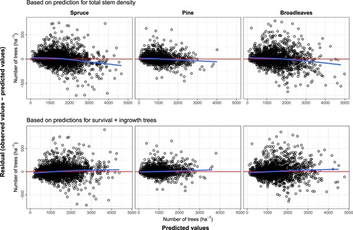
Table 5. Fit statistics comparison for total stem density when it is predicted using a model for the total number of trees versus when two sub-models are used to predict the survival and ingrowth trees.

Fit statistics	Spruce		Pine		Broadleaves
	N2	Nsur+ Ning	N2	Nsur+ Ning	N2	Nsur+ Ning
E	10.928	2.319	4.924	1.556	12.065	2.32
MAE	75.122	76.001	41.354	43.963	94.132	98.054
RMSE	115.701	114.614	69.108	69.482	142.359	143.261
R^2	0.9703	0.971	0.981	0.980	0.963	0.963

N₂, N_sur, and N_ing refer to the total number of trees, number of survival tree and number of ingrowth trees, respectively.

The parameters obtained for each species group for all components except ingrowth are given alongside the fit statistics in Table 6, where the parameter estimates are observed to be different for each species group, they are all significant at the α = 0.01 level. The fit statistics show that the coefficient of determination was at least 0.94 for the component models. The observed values are plotted against the predicted values in Figure 2. In all cases, the predictions follow the line of equality (identity line), with the residual error appearing evenly distributed on either side. A full examination of residual plots (Figure 3) also showed no apparent bias in the predictions. Further, Figure 4, illustrates the dominant height age curves for the common site indices (base age 40) for each species group, which fall within the ranges of height observations for those groups (see Table 1).

Figure 2. Observed vs. predicted values for the component models for each species group, the lines represent the line of equality in each case.

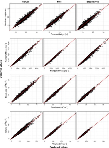
Figure 3. Residuals for the component models for each species group, the red lines represent the residuals equal to 0 andthe blue lines are the loess regression lines that can highlight any potential patterns that might exist amongst the residuals.

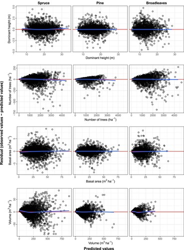
Figure 4. The dominant height age models illustrated using the common site indices (base age 40) for each species group.

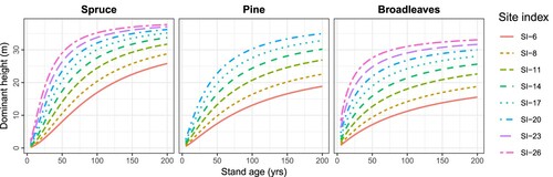
Table 6. Paramter estimates and fit statistics for the models applied to each species group.

	Spruce					Pine					Broadleaves
	H2	Nsur	N2	G2	V2	H2	Nsur	N2	G2	V2	H2	Nsur	N2	G2	V2
β1	39.5763 (1.3014)	0.6159 (0.0357)	1.5124 (0.0547)	0.4159 (0.0337)	0.2134 (0.0056)	43.6698 (4.0244)	0.17881 (0.0301)	0.6676 (0.0538)	0.5381 (0.0533)	0.4830 (0.0083)	36.6501 (4.1604)	0.4592 (0.0468)	1.1395 (0.0747)	0.2970 (0.1663)	0.5564 (0.0094)
β2	−396.3146 (137.7015)	−0.0312 (0.0024)	−0.00654 (0.0038)	2.0096 (0.1149)	1.0779 (0.0104)	−24.9476 (10.0290)	−0.0308 (0.0021)	0.0039 (0.0036)	0.96900 (0.0430)	0.9128 (0.0071)	−11.8787 (6.1456)	−0.0534 (0.0035)	−0.0162 (0.0056)	3.6124 (3.5470)	0.7667 (0.008)0
β3	1.6770 (0.0448)	1.0602 (0.0325)	1.4747 (0.0260)	0.7521 (0.1105)	1.0498 (0.0054)	1.2967 (0.0664)	0.0695 (0.1476)	0.8662 (0.0727)	4.1579 (0.3900)	0.9913 (0.0037)	1.0643 (0.1103)	0.9466 (0.0547)	1.2682 (0.0531)	0.2087 (0.4480)	1.0318 (0.0051)
β4					2.5148 (0.2536)					−1.6105 (0.2609)					−1.5229 (0.2541)
E	0.004	2.626	10.928	−0.067	0.497	0.0045	1.561	4.924	0.032	0.111	0.002	2.117	12.065	−0.138	0.445
MAE	0.590	48.467	75.122	1.112	12.653	0.441	26.192	41.354	0.680	6.915	0.668	57.370	94.132	0.978	4.62
RMSE	0.821	71.777	115.755	1.602	18.335	0.644	37.531	69.141	1.007	9.982	0.933	82.531	142.359	1.418	7.076
R^2	0.963	0.988	0.970	0.984	0.977	0.969	0.994	0.981	0.991	0.986	0.941	0.986	0.963	0.978	0.986

Refer to Tables 3 and 4, for the description of the variables.

The best combination of explanatory variables and their corresponding regression parameters to predict the ingrowth for each species group are presented in Table 7. Selected models provided better fit statistics in terms of VIF (< 2), AIC_w, AIC and loglik (see also Supplementary materials Figure 4) and all the parameter estimates were significant at the α = 0.05 level and showed biologically meaningful relation with ingrowth. Note that all the model equations, except the ones for the number of ingrowth trees have similar model forms for the three species group.

Table 7. Paramter estimates for the best fit selected to calculate the number and probability of ingrowth for each species group.

Species	Ingrowth count	Ingrowth probability
Spruce	$A=2.2919-0.3780\sqrt{G_1}$	$B=13.6210-3.0328\sqrt{D_1}-0.6868\sqrt{N_1}+0.1483\sqrt{D_1}\sqrt{N_1}$
	$A=0.5264-0.0889\sqrt{G_1}$	$B=7.6489-1.2823\sqrt{D_1}-0.5173\sqrt{N_1}+0.0915\sqrt{D_1}\sqrt{N_1}$
Broadleaves	$A=3.0411-0.6213\sqrt{D_1}$	$B=7.7009-1.6373\sqrt{D_1}-0.3349\sqrt{N_1}+0.5688\sqrt{D_1}\sqrt{N_1}$

N₁, D₁, and G₁ refer to the total stem number (ha⁻¹), quadratic mean diameter (cm), and basal area (m² ha⁻¹) of the stands at the beginning of the period.

Long-term projections

We applied the parameterized equations to visually examine long-term predictions for each component. Because the predicted number of trees when using two models for survival and ingrowth resulted in relatively less bias in the residuals, the long-term prediction of tree numbers is done for surviving trees. The total stem density for inclusion in basal area calculations is the sum of predicted survival and ingrowth at each step of the simulation. Figures 5–8 show these predictions for dominant height, survival, basal area, and total volume respectively. Each projection is illustrated for the species groups using examples of low, average, and high site indices relative to that group. Firstly, the dominant height appears to be reasonable, none of the heights exceed the heights of trees observed in Norway. The height growth is rapid, species-group dependent, and then slows with stand age, most apparently in the more productive sites (Figure 5). Secondly, the projected number of survived trees (Figure 6), which is site (plot) dependent, decreases with stand age. The rate of decline is more pronounced at higher site productivities. When accounting for the total number of trees (survival + ingrowth) in the model the predicted number of trees increases up to a maximum and then decreases by stand age (see Supplementary materials Figures 5 and 6). The peak occurs later (i.e. at older ages) in low site indices relative to higher site indices. The increase is more gradual and sustained in the low site indices relative to high site indices. Thirdly, basal area projections appear reasonable and biologically meaningful varying with species group and site productivity (Figure 7). The increase in basal area with stand age is more pronounced at early stand development stages and levels off, i.e. approaches an asymptote at higher stand ages depending on the site productivity. Lastly, the volume predictions (Figure 8) follow the same general trend as dominant height and basal area with volume growth rates and thus total volume varying with species group, site productivity, and stand age.

Figure 5. Long-term projections of stand dominant height using the model developed in this study for the three species groups and three site productivities (from left to right low, average, and high). The projections are for 100 years from the time of measured dominant height increment. SI = Site index at base age 40. The red dashed lines illustrate the general trendline for the overall means.

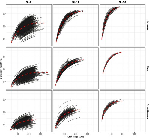
Figure 6. Long-term projections of the number of trees (only survival) using the model developed in this study for the three species groups and three site productivities (from left to right: low, average, and high). The projections are for 100 years from the time of measured increment. SI = Site index at base age 40. The red dashed lines illustrate the general trendline for the overall means.

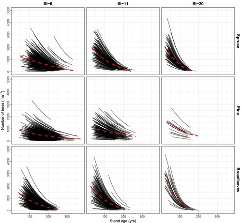
Figure 7. Long-term projections of stand basal area using the model developed in this study for the three species groups and three site productivities (from left to right: low, average, and high). The projections are for 100 years from the time of measured basal area increment. SI = Site index at base age 40. The stand basal area is calculated based on the total number of trees (survival + ingrowth). The red dashed lines illustrate the general trendline for the overall means.

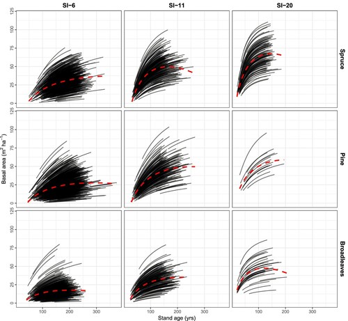
Figure 8. Long-term projections of stand volume using the model developed in this study and with observed dominant height, age, and basal area based on the total number of trees (survival + ingrowth) as input. Projections are illustrated for the three species groups and three site productivities (from left to right: low, average, and high). The projections are for 100 years from the time of measured increment. SI = Site index at base age 40. The red dashed lines illustrate the general trendline for the overall means.

Discussion

In this study, we successfully created stand-level growth and yield models for forests that do not strictly meet the criteria for simple even-aged, single-species stand structures. The main challenges we have met while developing the models for Norway’s forests include (1) the stands are not necessarily single species; (2) the age of the stands is not always certain or homogenous (i.e. trees in the same stand can have very different ages and the definition of even-aged does not apply); (3) there are a low number of repeated measurements (here only three); and (4) the data are unbalanced with respect to age and site productivity.

Our model development began with attempts to apply a model for productive, even-aged, and intensively-managed spruce forests (Allen et al. 2020) model to the spruce group data in our study. Presumably because of the differences between our forest type and the forest type for which the model by Allen et al. (2020) was developed for, the application of that model resulted in biased results for survival, basal area, and a noticeable overestimation of volume (see Supplementary materials Figures 1 and 2). The model by Allen et al. (2020) nonetheless served as a framework upon which our development took place. Further, considering the component equations, the models produced by Allen et al. (2020) were explicitly designed to incorporate silvicultural thinning, something that we could not parameterize with our data. Therefore, a simpler survival equation with three parameters (as opposed to five) was adopted here. Eventually, as a complimentary solution to correctly predict the total number of trees, we developed ingrowth equations for each species group. Adding the predicted ingrowth to the predicted number of survivals led to a reasonable estimation of total stem number. The stem density model could also effectively predict the total number of trees when both survival and ingrowth trees were considered as a whole. We also changed the dominant height and modified the basal area equations to ones that were more appropriate to our data. Volume is ultimately predicted based on stand age, basal area, and dominant height, such as is common practice (Borders 1989; Coble 2009; Zhao et al. 2015).

In traditional stand-level models’ ingrowth is assumed to be negligible (Clutter et al. 1983) and thus tree number is expected to decrease with increasing age. This was not the case in our dataset, particularly at lower site indexes. Approximately 35% of the plots in our dataset had an increase in the number of trees between the first and second measurements, because of higher number of ingrowth than mortality. For young stands this could be an artifact of the 5 cm DBH measurement threshold. Our data, as most NFIs, are left-censored because trees are only measured when they reached 5 cm DBH. For young stands this could mean that a relatively large number of trees could potentially appear between measurements if their DBH reach 5 cm between inventories (i.e. in reality they were always there, but too small to be measured). We tried to avoid this possible artifact by constraining our dataset to plots with a quadratic mean diameter of 8 cm or larger, but even then, an increase in the number of trees was not uncommon in our dataset, even for high site indices. However, most of the plots with an increase in the number of trees correspond to plots in low site index or in stands that have not reached maturity. The behaviour of our stem density model thus follows the increase in the number of trees observed for some of the studied plots and therefore differs from the traditional stand-level models in that it increases at young ages up to a peak and decreases afterward. Although the behaviour of the survival model followed the traditional stand-level models where the number of survival trees always decreases (e.g. Kuehne et al. 2022; Allen et al. 2020), there were no considerable differences between the two approaches we used to calculate the total stem density.

The limitations with our models are arguably more linked to the data than to the equations themselves. For example, it can be hard to set a meaningful age for some of the plots with more complex structures. This correlates to the observation that the potential bias in stand age is more pronounced for heterogenous plots of lower stand density where ingrowth occurs often and periodically. The stand age assigned to such uneven-aged plots thus is not necessarily meaningful. Given a significant change in forest management practices towards clearcutting since the 1950s in Norway, understocked, heterogenous plots are mostly found in higher age classes and for low site productivities. These plots, however, make up a considerable proportion of the data used in this study which presumably and in part explains the behaviour of the stem density equations developed here. As a result, deriving reliable dominant height models was specifically laborious and difficult. In addition, the comparatively small size of the studied NFI plots caused further difficulties and problems, particularly when developing meaningful ingrowth models.

We have drawn on comprehensive literature (e.g. Vanclay 1994; Liu et al. 1995; Diéguez-Aranda et al. 2005a; Anta et al. 2006; Burkhart and Tomé 2012) to examine the trends in other studies and we have found our models to be consistent with expected trends. Further, the NFI is a forest chronosequence that covers a large range of ages. Observations in the data used for this work span up to 236 years in stand age for spruce, 280 years for pine, and 165 years for birch. However, similarly to other models alike, long-term projections with our models are potentially subjected to large uncertainties.

A final limitation of the models that we present here is that within the data there are relatively few stands with medium or higher site indices, particularly at ages older than 80 years. Our data were positively skewed concerning the site index. There are very few stands older than 80 years with site indices greater than 11, whereas for example, spruce site indices range from 6 to 26 in Norway (Tveite and Braastad 1984). Ideally, we would have the full range of sites indices at every age. However, the NFI data represents the real structure of Norway’s forests where the most productive stands are harvested and regenerated. Ultimately, we do not propose the models that we present here as replacements of those created specifically for the more productive and well managed forests, where recent models for spruce (Allen et al. 2020) and pine (Kuehne et al. 2022) which allow for silvicultural treatments, are more appropriate and more reliable. Rather our models are specifically created to supplement those models in the many cases that they are not suitable.

We built models that use the stand age from the time of regeneration instead of the age at which the height of trees reaches 1.3 m, which is the traditional convention in Norway (Sharma and Brunner 2017; Tveite 1977), albeit our data were converted to age at regeneration from age at 1.3 m using species group-specific tables (e.g. Braastad 1980; Viken 2018). We believe it is important to consider the total age because it is more applicable to contemporary forest assessment and management. Further, simulations of forest growth from age zero are simpler to implement in forest design planning.

It is often recommended that models should be as simple as possible, robust, objective, unbiased, openly available, easy to employ, and facilitate decision support for forest management (Buchman and Shifley 1983; Vanclay 1994). We have followed this philosophy. Throughout our development of the models, the main intention was to capture the underlying mechanisms responsible for the growth and yield of stands belonging to any of the three species groups without explanatory variables that will not be available from even minimalist forest inventories. We have sought to keep our models simple and easy to implement by using a common set of equations, but with species group-specific parameters. We have investigated bias within the range of the data, and we have openly presented the models and discussed their uses and limitations. These models can, where appropriate, be implemented for the purposes of forest management in Norway.

We conclude that despite (1) using an approach originally developed for single species, even-aged forests and (2) the outlined limitations of the data studied, we were successful in deriving reliable systems of equations for predicting stand-level growth and yield of the structurally heterogenous forests found throughout Norway. We further found no major differences in the examined strategies of modelling change in stem density. While providing greater detail as compared to a model directly predicting stem density in general, predicting survival and ingrowth separately improved prediction accuracy only slightly. Overall, the models we produced are generally suitable for wider implementation. However, the proposed models are also of great potential to form the foundation for more sophisticated models, in which the influence of other factors such as natural disturbances, stand structure including species mixture, and any management practices can be included.

Acknowledgments

We are grateful to the many people who have been involved in collecting and maintain the data series used in this work. We also recognize the input of the following individuals, who contributed over the years to the development of the models for Norway and particularly Micky G. Allen II for making the materials for the latest developed growth and yield tool available to the authors. The first author acknowledges the support that was received through Statskog (the Norwegian State Forest).

Disclosure statement

No potential conflict of interest was reported by the author(s).

Additional information

Funding

The research was funded by NIBIO and Statskog.

References

- Allen MG, Antón-Fernández C, Astrup R. 2020. A stand-level growth and yield model for thinned and unthinned managed Norway spruce forests in Norway. Scandinavian Journal of Forest Research. 35(5-6):238–251. DOI: https://doi.org/10.1080/02827581.2020.1773525.
- Anastasov IZ. 2011. Evaluation of basal area projection models for unthinned and thinned central Appalachian hardwood forest stands. West Virginia University Libraries; [Accessed 3/8/2021]. https://researchrepository.wvu.edu/etd/3302.
- Anta MB, Dorado FC, Diéguez-Aranda U, González Á, Juan G, Parresol BR, Soalleiro RR. 2006. Development of a basal area growth system for maritime pine in northwestern Spain using the generalized algebraic difference approach. Can. J. For. Res. 36(6):1461–1474. DOI: https://doi.org/10.1139/x06-028.
- Bailey RL, Ware KD. 1983. Compatible basal-area growth and yield model for thinned and unthinned stands. Can. J. For. Res. 13(4):563–571. DOI: https://doi.org/10.1139/x83-082.
- Bates DM, Watts DG. 1988. Nonlinear regression analysis and Its applications. Hoboken: John Wiley & Sons, Inc (Wiley Series in Probability and Statistics). [Accessed 3/8/2021]. https://doi.org/http://doi.org/10.1002/9780470316757.
- Blingsmo K. 1984. Diameter increment functions for stands of birch, Scots pine, and Norway spruce. Ås: Norwegian Forest Research Institute. In 0333-001X, p. 22.
- Borders BE. 1989. Systems of equations in forest stand modeling. For Sci. 35(2):548–556. DOI: https://doi.org/10.1093/forestscience/35.2.548.
- Braastad H. 1966. Volumtabeller for bjørk. Meddelelser fra Det Norske Skogforsøksvesen. 21:23–78.
- Braastad H. 1974. Diametertilvekstfunksjoner for gran. Meddelelser fra Norsk Institutt for Skogforskning, 31/1.
- Braastad H. 1975. Produksjonstabeller og tilvekstmodeller for gran. Meddelelser fra Norsk Institutt for Skogforskning, 31/9.
- Braastad H. 1977. Tilvekstmodellprogram for bjørk. Rapport fra Norsk Institutt for Skogforskning, 1/77.
- Braastad H. 1980. Tilvekstmodellprogram for furu. Meddelelser fra Norsk Institutt for Skogforskning, 35/5.
- Braastad H. 1982. Naturlig avgang i granbestand. Rapport fra Norsk institutt for skogforskning 12/82.
- Brantseg A. 1967. Furu sønnafjells. Kubering av stående skog Funksjoner og tabeller. Meddelelser fra Det Norske Skogforsøksvesen. 22:695–739.
- Breidenbach J, Granhus A, Hylen G, Eriksen R, Astrup R. 2020a. A century of National Forest Inventory in Norway – informing past, present, and future decisions. For. Ecosyst. 7(1):46. DOI: https://doi.org/10.1186/s40663-020-00261-0.
- Breidenbach J, Waser LT, Debella-Gilo M, Schumacher J, Rahlf J, Hauglin M, et al. 2020b. National mapping and estimation of forest area by dominant tree species using sentinel-2 data. Can. J. For. Res. 51(3):1–15. DOI: https://doi.org/10.1139/cjfr-2020-0170.
- Buchman RG, Shifley SR. 1983. Guide to evaluating forest growth projection systems. Journal of Forestry. 81(4):232–254. DOI: https://doi.org/10.1093/jof/81.4.232.
- Burkhart HE, Tomé M. 2012. Modeling forest trees and stands. Dordrecht: Springer Netherlands. [Accessed 4/26/2021]. http://link.springer.com/https://doi.org/10.1007/978-90-481-3170-9.
- Cieszewski CJ, Bailey RL. 2000.: Generalized algebraic difference approach: theory based derivation of dynamic site equations with polymorphism and variable asymptotes. For Sci. 46(1):116–126. DOI: https://doi.org/10.1093/forestscience/46.1.116.
- Clutter JL, Fortson JC, Pienaar LV, Brister GH, Bailey RL. 1983. Timber management, A quantitative approach. New York: Wiley.
- Coble DW. 2009. A new whole-stand model for unmanaged loblolly and slash pine plantations in east texas. South J Appl For. 33(2):69–76. DOI: https://doi.org/10.1093/sjaf/33.2.69.
- Diéguez-Aranda U, Burkhart HE, Rodríguez-Soalleiro R. 2005a. Modeling dominant height growth of radiata pine (Pinus radiata D. Don) plantations in north-western Spain. For Ecol Manag. 215(1):271–284. DOI: https://doi.org/10.1016/j.foreco.2005.05.015.
- Diéguez-Aranda U, Castedo-Dorado F, Álvarez-González JG, Rodríguez-Soalleiro R. 2005b. Modelling mortality of Scots pine (Pinus sylvestris L.) plantations in the northwest of Spain. Eur J Forest Res. 124(2):143–153. DOI: https://doi.org/10.1007/s10342-004-0043-5.
- Dunn PK, Smyth GK. 1996. Randomized quantile residuals. J Comput Graph Stat. 5(3):236–244. DOI: https://doi.org/10.1080/10618600.1996.10474708.
- Eid T. 2001. Models for prediction of basal area mean diameter and number of trees for forest stands in south-eastern Norway. Scandinavian Journal of Forest Research. 16(5):467–479. DOI: https://doi.org/10.1080/02827580152632865.
- Eid T, Hobbelstad K. 2000.: AVVIRK-2000: A large-scale Forestry scenario model for long-term investment, income and harvest analyses. Scandinavian Journal of Forest Research. 15(4):472–482. DOI: https://doi.org/10.1080/028275800750172736.
- Elzhov TV, Mullen KM, Spiess A-N, Bolker B. 2016. minpack.lm: R Interface to the Levenberg-Marquardt Nonlinear Least-Squares Algorithm Found in MINPACK, Plus Support for Bounds. [Accessed 3/8/2021]. https://CRAN.R-project.org/package=minpack.lm.
- Hasenauer H, Burkhart HE, Amateis RL. 1997. Basal area development in thinned and unthinned loblolly pine plantations. Can. J. For. Res. 27(2):265–271. DOI: https://doi.org/10.1139/x96-163.
- Hobbelstad K, Hofstad O. 1988. AVVIRK3, a model for long-term forest planning. Rep. Norw. For. Res. Inst. 41:503–516.
- Hoen HF, Eid T. 1990.: A model for analysis of treatment strategies for a forest applying standvice simulations and linear programming [En modell for analyse av behandlingsalternativer for en skog ved bestandssimulering og lineær programmering]. Report. 9:90.
- Hoen HF, Gobakken T. 1997. Brukermanual for Bestandssimulatoren GAYA v1.20. Department of Forest Sciences, Agricultural University of Norway, 59 pp. Internal report.
- Hynynen J, Ojansuu R, Hökkä H, Siipilehto J, Salminen H, Haapala P. 2002. Models for predicting stand development in MELA system: Metsäntutkimuslaitos. http://urn.fi/URN:ISBN:951-40-1815-X.
- Kleiber C, Zeileis A. 2016. Visualizing count data regressions using rootograms. Am Stat. 70(3):296–303. DOI: https://doi.org/10.1080/00031305.2016.1173590.
- Kuehne C, McLean JP, Maleki K, Antón-Fernández C, Astrup R. 2022. A stand-level growth and yield model for thinned and unthinned even-aged Scots pine forests in Norway. Silva Fenn. 56(1). DOI: https://doi.org/10.14214/sf.10627.
- Kuehne C, Weiskittel AR, Fraver S, Puettmann KJ. 2015. Effects of thinning-induced changes in structural heterogeneity on growth, ingrowth, and mortality in secondary coastal douglas-fir forests. Can. J. For. Res. 45(11):1448–1461. DOI: https://doi.org/10.1139/cjfr-2015-0113.
- Lappi J. 1992. JLP: a linear programming package for management planning. Helsinki: Finnish Forest Research Institute. (Metsäntutkimuslaitoksen tiedonantoja).
- Liu J, Burkhart HE, Amateis RL. 1995. Projecting crown measures for loblolly pine trees using a generalized thinning response function. For Sci. 41(1):43–53. DOI: https://doi.org/10.1093/forestscience/41.1.43.
- McCullagh A, Black K, Nieuwenhuis M. 2017. Evaluation of tree and stand-level growth models using national forest inventory data. Eur J Forest Res. 136(2):251–258. DOI: https://doi.org/10.1007/s10342-017-1025-8.
- McTague JP, O'Loughlin D, Roise JP, Robison DJ, Kellison RC. 2008. The SOHARC model system for growth and yield of southern hardwoods. South J Appl For. 32(4):173–183. DOI: https://doi.org/10.1093/sjaf/32.4.173.
- Palahí M, Tomé M, Montero G, Miina J. 2002. Stand-level yield model for Scots pine (Pinus sylvestris L.) in north-east Spain. Investigación Agraria. Sistemas y Recursos Forestales. 11(2):409–424.
- Pienaar LV, Rheney JW. 1995. Modeling Stand level growth and yield Response to silvicultural treatments. For Sci. 41(3):629–638. DOI: https://doi.org/10.1093/forestscience/41.3.629.
- Pienaar LV, Shiver BD. 1986. Basal area prediction and projection equations for pine plantations. For Sci. 32(3):626–633. DOI: https://doi.org/10.1093/forestscience/32.3.626.
- Pukkala T, Lähde E, Laiho O. 2011. Using optimization for fitting individual-tree growth models for uneven-aged stands. Eur J Forest Res. 130(5):829–839. DOI: https://doi.org/10.1007/s10342-010-0475-z.
- Pukkala T, Lähde E, Laiho O. 2013. Species interactions in the dynamics of even- and uneven-aged boreal forests. Journal of Sustainable Forestry. 32(4):371–403. DOI: https://doi.org/10.1080/10549811.2013.770766.
- R Core Team. 2021. European Environment Agency. [Accessed 3/8/2021]. https://www.eea.europa.eu/data-and-maps/indicators/oxygen-consuming-substances-in-rivers/r-development-core-team-2006.
- Sharma M, Smith M, Burkhart HE, Amateis RL. 2006. Modeling the impact of thinning on height development of dominant and codominant loblolly pine trees. Ann. For. Sci. 63(4):349–354. DOI: https://doi.org/10.1051/forest:2006015.
- Sharma RP, Brunner A. 2017. Modeling individual tree height growth of Norway spruce and Scots pine from national forest inventory data in Norway. Scandinavian Journal of Forest Research. 32(6):501–514. DOI: https://doi.org/10.1080/02827581.2016.1269944.
- Sharma RP, Brunner A, Eid T, Øyen B-H. 2011. Modelling dominant height growth from national forest inventory individual tree data with short time series and large age errors. For Ecol Manag. 262(12):2162–2175. DOI: https://doi.org/10.1016/j.foreco.2011.07.037.
- Short E, Austin B, Harold E. 1992. Predicting crown-height increment for thinned and unthinned Loblolly pine plantations. For Sci. 38(3):594–610. DOI: https://doi.org/10.1093/forestscience/38.3.594.
- Socha J, Tymińska-Czabańska L, Grabska E, Orzeł S. 2020. Site index models for main forest-forming tree species in Poland. Forests. 11(3):19. DOI: https://doi.org/10.3390/f11030301.
- Strand L, Braastad H. 1967. Høydekurver for bjørk. Meddelelser fra det Norske Skogforsøksvesen. 22:291–302.
- Thapa R, Burkhart HE. 2015. Modeling stand-level mortality of loblolly pine (Pinus taeda L.) using stand, climate, and soil variables. For Sci. 61(5):834–846. DOI: https://doi.org/10.5849/forsci.14-125.
- Tomter SM, Hylen G, Nilsen JE. 2010. Norway. In: Tomppo E, Gschwantner T, Lawrence M, McRoberts RE, editors. National forest inventories: pathways for common reporting. Heidelberg, Dordrecht: Springer Science; p. 411–422. [Accessed 3/2/2021]. http://site.ebrary.com/id/10355992.
- Tveite B. 1967. Sambandet mellom grunnflateveid middelhøyde og noen andre bestandshøyder i gran- og furuskog. Meddelelser fra Det Norske Skogforsøksvesen. 22:483–538.
- Tveite B. 1976. Bonitetskurver for furu. Intern rapport. [Unpublished].
- Tveite B. 1977. Bonitetskurver for gran. Norsk Institute for Skogforskning. 33(1):88.
- Tveite B, Braastad H. 1984. Bonitering av gran, furu og bjørk. Ås: NLH, Norsk institutt for skogforskning.
- Vanclay JK. 1994. Modelling forest growth and yield: applications to mixed tropical forests. Wallingford: CAB International.
- Vestjordet E. 1967. Funksjoner og tabeller for kubering av stående gran. Meddelelser fra Det Norske Skogforsøksvesen. 22:539–574.
- Viken KO. 2018. Landsskogtakseringens feltinstruks: NIBIO (4(6)). www.xide.no.
- Wagenmakers E-J, Farrell S. 2004. AIC model selection using Akaike weights. Psychon Bull Rev. 11(1):192–196. DOI: https://doi.org/10.3758/BF03206482.
- Weiskittel AR, Hann DW, Kershaw JA, Vanclay JK. 2011. Forest Growth and Yield Modeling: vanclay/forest growth and yield modeling. Chichester: John Wiley & Sons, Ltd. [Accessed 4/26/2021]. https://doi.org/http://doi.org/10.1002/9781119998518.
- Woollons R. 1998. Even-aged stand mortality estimation through a two-step regression process. For Ecol Manag. 105:189–195. doi:https://doi.org/10.1016/S0378-1127(97)00279-X
- Yue C, Kohnle U, Hein S. 2008.combining tree- and stand-level models: A new approach to growth prediction. For Sci. 54(5):553–566. DOI: https://doi.org/10.1093/forestscience/54.5.553.
- Zeileis A, Kleiber C. 2016. countreg: Count Data Regression. R package version 0.1-5/r106. http://R-Forge.R-project.org/projects/countreg/.
- Zhao D, Kane M, Markewitz D, Teskey R, Clutter M. 2015. Additive tree biomass equations for midrotation Loblolly pine plantations. For Sci. 61(4):613–623. DOI: https://doi.org/10.5849/forsci.14-193.