Multispectral analysis of multimodal images

Abstract

Introduction. An increasing number of multimodal images represent a valuable increase in available image information, but at the same time it complicates the extraction of diagnostic information across the images. Multispectral analysis (MSA) has the potential to simplify this problem substantially as unlimited number of images can be combined, and tissue properties across the images can be extracted automatically. Materials and methods. We have developed a software solution for MSA containing two algorithms for unsupervised classification, an EM-algorithm finding multinormal class descriptions and the k-means clustering algorithm, and two for supervised classification, a Bayesian classifier using multinormal class descriptions and a kNN-algorithm. The software has an efficient user interface for the creation and manipulation of class descriptions, and it has proper tools for displaying the results. Results. The software has been tested on different sets of images. One application is to segment cross-sectional images of brain tissue (T1- and T2-weighted MR images) into its main normal tissues and brain tumors. Another interesting set of images are the perfusion maps and diffusion maps, derived images from raw MR images. The software returns segmentations that seem to be sensible. Discussion. The MSA software appears to be a valuable tool for image analysis with multimodal images at hand. It readily gives a segmentation of image volumes that visually seems to be sensible. However, to really learn how to use MSA, it will be necessary to gain more insight into what tissues the different segments contain, and the upcoming work will therefore be focused on examining the tissues through for example histological sections.

In the last decades we have seen an increase in the number of image modalities for medical use. Of the modalities with tomographic capabilities we have CTs, MRs, ultrasound apparatus, SPECT and PET, and at many institutions all these are available. In recent years the awareness of the need of multimodal imaging has been growing, and for this reason more and more images are acquired for each patient. It is recognized that one modality cannot always reveal all the necessary information, and we use different modalities that will complement each other.

An increasing number of multimodal images represent a valuable increase in available image information, but at the same time it complicates the extraction of diagnostic information across the images. The first step towards efficient use of the images is registration of the images. In many cases this is a difficult task, but it is nonetheless a very important one. Secondly we need some visualization technique that shows the information in two or more images simultaneously. This could be accomplished with simple overlay techniques, e.g. one image on top of the other with user adjustable transparency or more advanced 3D rendering techniques. With such tools in place the examiner can see where a region of interest in one image is located relative to a region in another image. Still, such a solution has its severe limitations with regards to image analysis.

Visualization of more than two images simultaneously is difficult to do without confusing the observer, and today we often encounter a situation with at least three images. Another issue with regards to information extraction lies in going from qualitative to quantitative information. Traditionally the radiologist draws regions of interest in one image or possibly in an image with an additional image overlay, and he does this based on what he can visually observe with the image representation (linear vs. logarithmic, window leveling etc) he has chosen to use. Preferably the process of defining regions should be done using all available and useful image information simultaneously and possibly in an objective manner based on quantitative measures.

Multispectral analysis (MSA) is a set of algorithms that has the potential to simplify the problem of information extraction from multiple images, and in a quantitative way. An unlimited number of images may be used for input to the algorithms, and tissue properties across the images can be extracted automatically. In this article we give a brief introduction to MSA before we describe a software solution for MSA analysis with the algorithms included and the solution chosen for the graphical user interface. We also present a few examples with a view towards specific applications.

Materials and methods

An introduction to MSA

MSA was originally developed for applications using satellite images acquired with cameras sensitive to different photon spectra, hence the name “Multispectral”. A typical problem was classification of landscapes on the earth imaged from the satellites [1]. The statistical methods developed for these purposes are, however, not specifically engineered for satellite applications; on the contrary they are very general and may be used for about any segmentation problem consisting of multiple images acquired of the same object. In the last decades a number of articles have emerged describing the use of MSA for analysis of medical images [2–10].

The basic idea of multispectral analysis is to form feature vectors consisting of pixel values in the individual images. Assuming that the images have the same image dimensions, have the same resolution and that they are properly registered, denote the image element (i, j) of image m, as . The feature vector for the position (I, j) is denoted by . The analysis is performed using these vectors as input, and thus the information from all the K images is used simultaneously. What we want to do is to somehow divide the set of vectors into classes consisting of vectors that, according to some measure, belong together, and in this way perform a segmentation of the images. What we mean with “belong together” is a matter of choosing an algorithm that we find appropriate for the specific task.

MSA algorithms can be either supervised or unsupervised. The supervised rely on prior information about the classes, class descriptions, and a vector is classified to the class with the class description that best fits the vector. The class descriptions can be formulated in different ways, but generally one can say that they are probability density functions, and a classification of a vector usually means to assign the vector to the class that minimizes the probability for misclassification.

The class descriptions can furthermore be parametric or nonparametric. Using a parametric description a large set of sample vectors have been used to find the parameters of the statistical models, the class descriptions, which are believed to describe the data appropriately. New input vectors are then classified according to these class descriptions. A frequently used statistical model is the multinormal distribution, the generalization of the normal distribution to a multidimensional space.

A nonparametric distribution relies on class descriptions consisting of sample vectors believed to be representative for the class. The classification implies a comparison of the input vector with the sample vectors belonging to the different classes. Obviously nonparametric methods are much slower than the parametric as the former involve a comparison with a large number of sample vectors while using parametric methods one only has to calculate the probabilities for the vector belonging to the different classes using functional expressions.

The advantage of the nonparametric classifiers is that we don't have to assume anything about the true distribution of vectors within a class. Using a parametric distribution one has to choose a functional form for each class, for example the multinormal distribution, and if this function does not fit the data particularly well the classifier may not work very well meaning that an unsatisfactorily high fraction of the vectors will be misclassified.

It is possible to do a post processing step that includes the information of the surrounding pixels, contextual classification. In effect this step will increase the probability for classifying the pixel in question to the classes of the surrounding pixels, resulting in smoother segmentations as transitions from one class to another are discouraged. One could argue that this will introduce an artificial smoothness in the images, but in the presence of transitional effects in the input images, like partial volume effects, it is well motivated.

Unsupervised classifiers use no prior information about the classes. Usually the algorithm is told how many classes there should be, but there exist algorithms that also determine the number of classes. Unsupervised classifiers are appropriate if sample vectors are not available for the construction of class descriptions, but also when class descriptions are changing between image sets. That can be the case when normalization is changing, for example if different imaging machines are used. Unsupervised classification is also useful if the user does not know prior to construction of class descriptions what classes are present in the images. In that case the result of the unsupervised classification can be used for the formation of the class descriptions. For an illustration of the different classification alternatives, see Figure 1. See [11] for a general introduction to multivariate image analysis.

Figure 1.  Main alternatives for MSA.

The software solution

The goal of the project was to develop a general tool for MSA where all the alternatives in Figure 1 should be covered with one or more alternative algorithms. Furthermore, the software should be easy to use with an intuitive user interface in all the steps towards a classified output. Finally, it is important with a good tool for the presentation and post processing of the results.

The MSA algorithms implemented in the software

At present the software contains two algorithms for supervised and two for unsupervised classification. For supervised classification there is one parametric and one nonparametric, a Bayesian classifier using multinormal class descriptions and the well known k-nearest-neighbors (kNN) classifier, respectively. The Bayesian classifier [12] is based on classical Bayesian decision theory meaning that one operates with (1) Apriori probabilities and (2) Aposteriori probabilities. The Apriori probability P(C_k) indicates the probability for a pixel to belong to class k that is estimated/guessed before the vector of pixel values is introduced. The Aposteriori probability, P(C_k|V), is the probability of a pixel belonging to class k given the feature vector V of the pixel, and it is this probability which we want to find with MSA. With Bayesian decision theory this is given by1 Using this expression for the Aposteriori probability the misclassification rate is minimized.The probability of finding the feature vector V given that the pixel belongs to class C_k, p(V|C_k), is given by the class description with parameters estimated from sample vectors. In this software it was chosen to use a multinormal model:2 where µ_k is the mean vector of class k, Σ_k is the covariance matrix and d is the dimension of the vectors equaling the number of input images.

The nonparametric supervised classifier implemented in this software package is the well known kNN-algorithm. Contrary to the algorithm described above this algorithm simply uses sample vectors that are believed to be representative for the different classes. For each input vector V the k vectors of the total pool of sample vectors (the sample vectors for all the classes) closest to V are found. Then the pixel is assigned to the class that contains the highest number of those k sample vectors.

A potential problem with this algorithm as formulated above is related to the number of sample pixels representing the different classes. If those numbers are not proportional to the true size of the class, this could lead to misclassifications in the area of vector space where classes overlap. For this reason we chose to do a normalization consisting of a division with the sample sizes and a multiplication with the Apriori probabilities described above.

The two unsupervised classifiers are the k-means and an Expectation-Maximization (EM) algorithm [13]. The former is a classical clustering algorithm used on a wide range of applications, appreciated for its robustness and simplicity. It starts with an initial guess for the k mean vectors for the k classes we want to find (Be aware of the difference between the k's in the kNN and the k-means algorithms!). Then all the input vectors are assigned to the closest of the mean vectors, and new mean vectors are calculated from the vectors assigned to the different classes. Thereafter an iterative process is started where each iteration consists of (1) moving vectors to the nearest mean vector and (2) recalculate the mean vectors.

Involved in this algorithm is a distance measure, and it is not obvious how to define it. The simplest solution is to use the Euklidian distance, but this is not appropriate when the elements of the input vectors (meaning the pixels of the different input images) span intervals of different lengths. We chose to normalize using the standard deviation of the input images.

The second unsupervised algorithm is an EM-algorithm [13] implemented with multinormal probability distributions. It seeks to find multinormal class descriptions (like the descriptions for the Bayesian supervised algorithm) that maximizes the log-likelihood of finding the input vectors present in the input images, and it is therefore special as a supervised algorithm in that it actually returns parametric class descriptions. This is very useful as it then can be used for establishing class descriptions that can be used later for supervised classification.

In short the algorithm works iteratively with two steps in each iteration: 1) With the present class descriptions, calculate the probabilities of observing the input vectors using Equation 1 and 2 and 2) increase the log-likelihood by an adjustment of the class descriptions. In step 2 the Apriori probabilities are also updated. The maximization is done going in the direction of the derivatives of the log-likelihood, and it is therefore not guaranteed that one ends up in a local maximum. For this reason we implemented this with a possibility for using a momentum, meaning that the adjustments to the parameters are a weighted sum of the former step and the step calculated from the derivatives.

Often when doing unsupervised classification one does not know how many classes one should look for, and in that situation it may be useful to use some objective criterion for the choice of number of classes. One such criterion is the Minimum Description Length (MDL) criterion [14]. It weighs the log-likelihood of the fit of the model (consisting of the class descriptions) against the complexity of the model which in this case is given by the number of classes, N, and the total number of parameters, J:3 λ is a constant scalar equal to 3/4.With the algorithms returning probabilities for a vector belonging to the different classes, it is possible to do a post processing step which includes contextual information. In this software package we have implemented Haslett's method [15]. The Aposteriori probability is modified by multiplication with the factorwhere Q is a normalization constant and , V_x is the feature vector of neighbor X and is the probability of observing a class l pixel next to a class k pixel. It was assumed that the transitional probabilities are the same in all directions. However, we did take into account that the distance between the voxels in the different directions may be different. If the distance is very large the pixels are not correlated, and thereby the transitional probabilities must all be equal. In the other extreme, if the distance is very small must be close to 1 if l=k and close to 0 if l≠k.

The software solution

The software was developed in C + + using CodeGear™ RAD studio (CodeGear, CA, USA), and was embedded into an already existing software package (nordicICE, NordicImagingLab, Bergen, Norway) that contains useful functionality with regards to reading and writing of images, some image analysis tools and most important, capabilities for drawing and handling of regions of interest. It was designed with focus on the different tasks involved in MSA: Extraction of feature vectors for the generation of class descriptions, manipulation and saving/reading of the descriptions, running the MSA algorithms and finally presenting the results. The functionality was implemented in a modern GUI interface making it easily accessible.

In this software there are three possibilities for generating class descriptions: 1) Using ROIs to extract feature vectors from which class descriptions are generated, 2) doing an unsupervised classification and using the resulting segmentations and 3) defining a parametric description by manually entering parameter values.

Irrespective of the method chosen for the generation of class descriptions, the class descriptions are put into a tree structure. Several classes can be put under the same branch, and in later supervised classifications these classes will be treated as one with regards to the final segmentation. This means that we in effect allow for multimodal descriptions in the case of multinormal class descriptions. From the users point of view this arranging of the classes is done by actually moving the class around in a visual tree structure. The need for grouping together classes frequently comes up with unsupervised classification, and is very useful for preparation of class descriptions for supervised classification. Both the parametric class descriptions and the nonparametric are dealt with in the same tree. This is useful as the software also has capabilities for converting multinormal classes into sample vectors and oppositely, estimating the parameters of a multinormal class from a set of sample vectors. In the same control sheet the user may also change the class parameters or change the color with which the class will appear in the segmented image.

The algorithms themselves are started by clicking at buttons in the GUI. The algorithms are organized into sheets according to what kind of class descriptions they take as input. After a classification algorithm has been run two windows appear which show the segmented image and the Aposteriori probability distributions which the segmentation was based on. The color coding is controlled in the above described class description control sheet. The segmented images are connected to the geometrical information from the input images, and they may therefore be put on top of the input images as overlays.

Results

A software solution for general MSA has been developed. It has been tested on a number of different combinations of MR images, both structural T1 and T2 images, but also on derived images like perfusion maps and diffusion maps. We will here present a few case studies.

Structural images of the brain

T2 and T1 MR images in combination give a lot of structural information, and is frequently used for examinations of the brain due to the excellent soft tissue contrast. As a first test of the software segmentations were performed on simulated data found at http://www.bic.mni.mcgill.ca/brainweb [16–19]. We used T1 and T2 images with slice thickness equal to 1mm and with 3% noise. The input for the generation of these data is tissue composition maps that give the fractions of the different types of tissue in the individual voxels. However, the maps also constitute ground truth for the segmentations, and thus serve as a means for validation of the methods.

The number of tissue types used in the MR simulations was 9 (CSF, white and grey matter, glial matter fat, connective tissue, skull, skin and a skin/muscle mixture), and we therefore used 9 classes in an unsupervised classification using the EM algorithm. Furthermore we created class descriptions, both multinormal and non-parametric (using only those pixels that contained only one type of tissue) that were used in supervised classifications with the Bayesian classifier and the kNN classifier.

For the large classes like CSF, white and grey matter and skull, the unsupervised classifier reproduced the ground truth to a large extent (Figure 2). However, for the other classes the parameter space was not generally subdivided into the tissue classes. For example, the glial matter overlaps in parameter space with the grey matter, and these two tissue types are not separated into individual classes.

Figure 2.  Segmentation results with simulated MR data. The three top left images are without postprocessing, the three to the right are with postprocessing. The top images are the results of unsupervised segmentation with the EM-algorithm with 9 classes, the images below show segmentation using the Bayesian classifier with multinormal class descriptions, the third row are the results with kNN classification. The bottom image represents the ground truth as it shows the tissue type making up the major fraction of the individual voxels. The color coding is the same in all images. The orange in the centre of the brain is glial matter. Outside the brain there is skull, muscle, fat, connective tissue and skin.

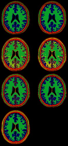
The Bayesian classifier had a problem with the separation of white matter from fat and connective tissue. Furthermore, some of the grey matter was classified as glial matter showing that some of the class descriptions overlapped using a multinormal class description. The segmentations delivered by the kNN classifier were to a much higher degree in accordance with the true tissue volumes. White matter was not mixed up with fat and connective tissue, and grey matter was not classified as glial matter. This shows that the non-parametric descriptions are much more robust than the parametric. However, only very few of the glial matter pixels were correctly classified as such. For all the segmentations performed with the simulated data, and in particular for the supervised algorithms, post-processing with Hasletts’ method improved the results.

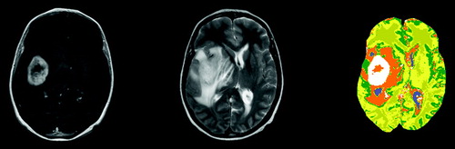
In Figure 3 the input images of a brain with a tumor is shown together with a segmentation. A contrast agent was administered to the patient before acquisition of the T1 image to enhance areas with a leaky blood brain barrier, typically seen in tumors. For this segmentation the unsupervised EM algorithm was used with 6 classes. In the segmented image we see that the abnormal area is divided into three parts. These are probably a central necrotic region, the viable tumor tissue and edema surrounding the tumor tissue, typical of high grade tumors.

Figure 3.  T1, T2 and the segmented image of a brain with a tumor.

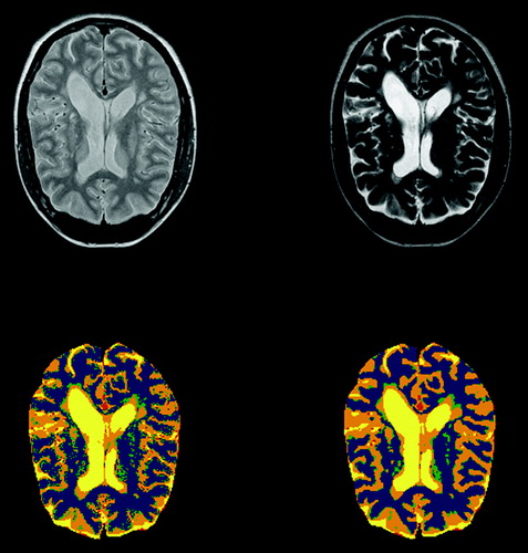
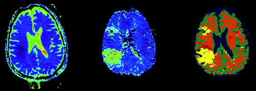
Figure 4 shows a segmentation of an MS-patient's brain, clearly showing the lesions typical of this patient group. The input images here were T2 and proton density MR images. This segmentation was done using the unsupervised EM-algorithm with 8 classes. Two of the classes were grouped together as CSF, 2 as white matter and 2 as gray matter. The two remaining classes are blood vessels and the abnormal lesions. In Figure 4 results with and without post processing with Haslett's method are shown. We see a very much smoother image without small speckles using post processing.

Figure 4.  On top, T2 and proton density images of an MS patient. The lower images show segmentation without and with postprocessing with Hasletts method.

The last application shown here is an MSA of a stroke patient (Figure 5). Input images are an Apparent Diffusion Coefficient (ADC) map and a Mean Transit Time (MTT) map. An ADC map shows how freely the water molecules may move within the tissue while the MTT map shows how long time the blood resides in the tissues. The latter is derived from a time series of images acquired after the injection of a contrast agent. This segmentation was done with a supervised algorithm with predefined class descriptions which was found by defining ROIs of the different tissue types.

Figure 5.  A stroke patient. Images are ADC map, MTT map and the segmented image.

For the treatment of stroke patients it is the penumbra region that is of interest. The penumbra is the mismatch between the lesions in the ADC and MTT maps, and it is believed that this is an area that can be saved. In the segmented image the penumbra has red color, and we see that for this patient the penumbra region is relatively small.

Discussion

The increasing number of images available for each patient calls for more image analysis tools, and MSA is one such tool. It has the ability to group together feature vectors that in some sense belong together, depending on the algorithm chosen. The idea is that the combination of several characteristics together gives a better opportunity to see different tissue types. An obvious example is the penumbra region of a stroke patient which cannot be defined in either the ADC or the MTT but in a combination of the two.

The implementations of the algorithms in this software allow for segmentations in both 2D images and 3D volumes, and as such the software can be useful for applications like external radiotherapy planning or surgery. Radiotherapy is today more and more dependent on image information and especially with regards to exploiting the possibilities of IMRT it is crucial with accurate knowledge about the extent of the cancerous tissue. For this purpose oncologists request functional imaging by means of PET or MR, and the need for objective methods for tumor delineation is present.

The first results suggest that MSA is a valuable tool for image analysis when multimodal images are available. It gives a segmentation of image volumes that by visual inspection seems to be sensible, and the inspection of the results obtained with simulated data supports this. However, do we really know that the segmentation really divides the volumes into the appropriate tissue types when we are working with real data? With supervised classification someone must have created the class descriptions with an idea that the feature vectors included were representative of the classes, but still, the supervised classifiers still rely on good class descriptions. If the descriptions were created by extracting vectors from an area defined by a ROI, the ROIs were probably drawn around areas that were very typical for the tissue in question. However, this opens up for missing the more atypical vectors of the tissues, leading to class descriptions with too small widths. Furthermore, the danger of using a bad setting for the window leveling or some other display parameter may cause errors in the class descriptions.

With unsupervised classification we let the algorithms define the classes, and in effect it means to let the algorithm search for densely populated volumes in feature vector space. We seek models that best fits the data. This is not a guarantee of defining the classes correctly. We never know that a class should have a Gaussian shape, the true class descriptions could have any form.

For these reasons it is important with some sort of validation of the MSA algorithms up against what is available of ground truth. We have looked at simulated data, but ideally we should use histological tissue sections examined under a microscope which are registered with the images [20]. In the continuation of this project this is what will look into. We want to find tissue signatures established through careful examinations of tissue sections.

Another issue that we will start looking into is the normalization problem. Images are in general not quantitative measures of some physical property unless a careful normalization procedure is undertaken. With predefined class descriptions this constitutes a problem which has to be dealt with for successful classification. Possible solutions here could be to use an easily identifiable tissue with known mean values and use this to normalize the rest of the image. However, this is only doable if the tissue property does not vary much between individuals.

In conclusion we have constructed a tool for MSA that mathematically works as it should. We have implemented a set of algorithms that covers most needs in MSA, and given it a user friendly interface. The case studies shown here is a proof of principle of the potential of the concept, but to really make it a useful tool it is necessary to establish reliable class descriptions for different tissue types.

Acknowledgements

This work was funded by a research grant to R.G. from the Bergen Research Foundation, Norway. The work was done in collaboration with NordicImagingLab Inc., Bergen, Norway.

References

- Richards J. Remote Sensing Digital Image Analysis. Springer-Verlag, New York 1986
- Amato U, Larobina M, Antoniadis A, Alfano B. Segmentation of magnetic resonance brain images through discriminant analysis. J Neurosci Meth 2003; 131: 65–74
- Carano RAD, Ross AL, Ross J, Williams SP, Koeppen H, Schwall RH, Van Bruggen N. Quantification of tumor tissue populations by multispectral analysis. Magn Reson Med 2004; 51: 542–51
- Chan DY, Cheng HY, Hsieh HL. Tissue separation in MR images-from supervised to unsupervised classification. J Vis Comm Image Represent 2004; 15: 185–202
- Fletcher-Heath LM, Hall LO, Goldgof DB, Murtagh FR. Automatic segmentation of non-enhancing brain tumors in magnetic resonance images. Artif Intell Med 2001; 21: 43–63
- Henning EC, Azuma C, Sotak CH, Helmer KG. Multispectral quantification of tissue types in a RIF-1 tumor model with histological validation. Part I.Magn Reson Med 2007; 57: 501–12
- Henning EC, Azuma C, Sotak CH, Helmer KG. Multispectral tissue characterization in a RIF-1 tumor model: Monitoring the ADC and T-2 responses to single-dose radiotherapy. Part II. Magn Reson Med 2007; 57: 513–9
- Tiwari P, Madabhushi A, Rosen M. A hierarchical unsupervised spectral clustering scheme for detection of prostate cancer from magnetic resonance spectroscopy (MRS). Med Image Comput Comput Assist Interv Int Conf Med Image Comput Comput Assist Interv 2007; 10: 278–86
- Wu YT, Chou YC, Guo WY, Yeh TC, Hsieh JC. Classification of spatiotemporal hemodynamics from brain perfusion MR images using expectation-maximization estimation with finite mixture of multivariate Gaussian distributions. Magn Reson Med 2007; 57: 181–91
- Zavaljevski A, Dhawan AP, Gaskil M, Ball W, Johnson JD. Multi-level adaptive segmentation of multi-parameter MR brain images. Comp Med Imaging Graph 2000; 24: 87–98
- Geladi P, Grahn H. Multivariate Image Analysis. John Wiley & Sons, Chichester 1996
- Lee P. Bayesian statistics: An introduction. Oxford University Press, New York 1989
- McLachlan G, Krishnan T. The EM algorithm and extensions. John Wiley & Sons, New Jersey 1997
- Schwarz G. Estimating dimension of a model. Ann Stat 1978; 6: 461–4
- Haslett J. Maximum-Likelihood Discriminant-Analysis on the plane using a Markovian model of spatial context. Pattern Recogn 1985; 18: 287–296
- Cocosco C, Kollokian V, Kwan RK-S, Evans A. BrainWeb: Online interface to a 3D MRI simulated brain database. In International Conference on Functional Mapping of the Human Brain. Copenhagen: 1997. p S425.
- Collins DL, Zijdenbos AP, Kollokian V, Sled JG, Kabani NJ, Holmes CJ, et al. Design and construction of a realistic digital brain phantom. IEEE Trans Med Imag 1998; 17: 463–8
- Kwan RKS, Evans AC, Pike GB. An extensible MRI simulator for post-processing evaluation. In: Visualization in biomedical computing. Lecture Notes in Computer Science. 1996; 1131: 135–40
- Kwan RKS, Evans AC, Pike GB. MRI simulation-based evaluation of image-processing and classification methods. IEEE Trans Med Imaging 1999; 18: 1085–97
- Zhan Y, Ou Y, Feldman M, Tomaszeweski J, Davatzikos C, Shen D. Registering histologic and MR images of prostate for image-based cancer detection. Acad Radiol 2007; 14: 1367–81