Influence of gray level discretization on radiomic feature stability for different CT scanners, tube currents and slice thicknesses: a comprehensive phantom study

Abstract

Background: Radiomic analyses of CT images provide prognostic information that can potentially be used for personalized treatment. However, heterogeneity of acquisition- and reconstruction protocols influences robustness of radiomic analyses. The aim of this study was to investigate the influence of different CT-scanners, slice thicknesses, exposures and gray-level discretization on radiomic feature values and their stability.

Material and methods: A texture phantom with ten different inserts was scanned on nine different CT-scanners with varying tube currents. Scans were reconstructed with 1.5 mm or 3 mm slice thickness. Image pre-processing comprised gray-level discretization in ten different bin widths ranging from 5 to 50 HU and different resampling methods (i.e., linear, cubic and nearest neighbor interpolation to 1 × 1 × 3 mm³ voxels) were investigated. Subsequently, 114 textural radiomic features were extracted from a 2.1 cm³ sphere in the center of each insert. The influence of slice thickness, exposure and bin width on feature values was investigated. Feature stability was assessed by calculating the concordance correlation coefficient (CCC) in a test-retest setting and for different combinations of scanners, tube currents and slice thicknesses.

Results: Bin width influenced feature values, but this only had a marginal effect on the total number of stable features (CCC > 0.85) when comparing different scanners, slice thicknesses or exposures. Most radiomic features were affected by slice thickness, but this effect could be reduced by resampling the CT-images before feature extraction. Statistics feature ‘energy’ was the most dependent on slice thickness. No clear correlation between feature values and exposures was observed.

Conclusions: CT-scanner, slice thickness and bin width affected radiomic feature values, whereas no effect of exposure was observed. Optimization of gray-level discretization to potentially improve prognostic value can be performed without compromising feature stability. Resampling images prior to feature extraction decreases the variability of radiomic features.

Introduction

Extraction of quantitative imaging features, also called radiomics [1], has become an additional source of information for the development of prognostic and predictive models [2–7]. The total number of features that can be calculated is almost unlimited, especially if filter-based features (e.g., Laplacian of Gaussian or wavelet) are also taken into consideration. To incorporate such large numbers of features in prognostic and predictive models, multiple independent and multi-centric datasets are needed for training and validation. However, recent literature shows that there are some challenges to overcome [8].

Several studies already showed that radiomic feature values are influenced by image acquisition and reconstruction settings, like slice thickness and exposure [2,9–13]. For instance, Mackin et al. [13] scanned a phantom with ten unique inserts using different acquisition parameters on computed tomography (CT) scanners of four manufacturers. They demonstrated that the variability in textural features calculated on the phantom scans can be in the same order of magnitude as the variability seen in non-small cell lung cancer patients (NSCLC). Using the same phantom, Shafiq-ul-Hassan et al. [12] investigated voxel-size dependency of radiomic features and found that this dependency can be minimized by resampling to a nominal voxel size or by normalizing the voxel size. Next to that, they found that gray-level dependency also can be reduced by normalization. Since multi-centric data usually are acquired with different CT-scanners using institutional scan protocols, the lack of statistical power in validation datasets might, therefore, be attributed to the different acquisition settings.

In the current study, we investigated the variability in radiomic feature values for scans with different slice thicknesses, different exposures and from different CT-scanners and performed a test-retest analysis using the same texture phantom as Mackin et al. and Shafiq-ul-Hassan et al. [12,13]. In addition to these former studies, we used a more extensive radiomic features dataset, different scanner types and focused more on the influence of gray-level discretization and resampling of voxel size on interchangeability of radiomic features. Furthermore, we compared the variability of radiomic features values derived from the phantom with those derived from two independent non-small cell lung cancer (NSCLC) patient datasets, to investigate the comparability of the phantom inserts to clinical CT-scans.

Material and methods

Image acquisition

The Credence Cartridge Radiomics phantom (CCR), previously described by Mackin et al. [13], consists of an acrylic case with ten different inserts with different textures and was scanned on nine different CT-scanners. We focused on the shredded rubber insert, because the CT-properties of this insert are most similar to tumors [13].

An overview of all scanners and settings is provided in Table 1. The scans were reconstructed using two different slice thicknesses per scanner. For the ‘H’ scanner, the ‘B’ scanner and the ‘O’ scanner the increment as well as the slice thickness was 1.5 mm or 3 mm. For the other scanners the increment was 1 mm for scans with a slice thickness of 1.5 mm (scanner ‘S’ had a slice thickness of 2 mm instead of 1.5) and 2 mm for the scans with a slice thickness of 3 mm. The reconstructed field of view was 500 mm for all scans.

Table 1. Overview scanners and per scanner exposure time, convolution kernel, tube current, focal spot size and collimation.

Hospital	Vendor	Model	Coding	Exposure time (ms)	Convolution kernel	Tube Current (mA)	Focal spot size (mm)	Collimation (# * mm)
1	Siemens	SOMATOM Definition Flash	Fl	500	B31f	128, 160, 296, 592	1.2	64 * 0.6
	Philips	Brilliance 64	P	561	B	61, 91, 119, 148, 274	1.0	64 * 0.6
2	Siemens	Biograph 40	B	500	B31f	40, 60, 80	1.2	24 * 1.2
	Siemens	SOMATOM Confidence RT Pro	C	1000	B31s	26, 39, 52, 66, 121	1.2	32 * 0.6
	Siemens	SOMATOM Sensation Open	O	500	B31f	60, 80, 100	1.2	24 * 1.2
3	Siemens	SOMATOM Definition Flash	L	500	B31f	64, 96, 128, 162, 296, 594	1.2	64 * 0.6
4	Siemens	SOMATOM Definition AS+	V	500	B31f	64, 96, 128, 162, 298, 594	1.2	64 * 0.6
5	Siemens	Biograph 16	H	500	B31f	40, 60, 84, 112, 140, 216, 274	0.7	16 * 0.75
6	Philips	Gemini TF 16	S	534	B	58, 88, 114, 143, 266, 497	1.0	16 * 1.5

All scans were performed with a tube voltage of 120 kVp and a pitch of 1.0. The aim was to scan the phantom with the same range of CT-dose index (CTDI) settings [2.17, 3.26, 4.32, 5.43, 10, 20 mGy], but due to hardware (e.g., the risk of overheating) and software limitations (i.e., not all exposures could be set) not all CTDIs could be obtained for all scanners. Philips scans were reconstructed using the B kernel and Siemens scans using the B31f or B31s kernel.

For test-retest purposes, two subsequent CT-scans were acquired on the ‘B’ and the ‘O’ scanner. The phantom was kept in place on the table without changing anything in between, meaning that no other parameters than scanner output fluctuations could have influenced the images.

Feature extraction

A spherical region of interest (ROI) with a volume of 2.1 cm³ was contoured using Mirada RTx (Mirada RTx 1.6, Mirada Medical, Oxford, UK) in the center of every insert. Moreover, for test-retest purposes, the ROI was shifted to the right and downwards. Supplementary Material A shows an example CT image of the phantom in which the ROIs are indicated in the rubber insert.

One hundred and fourteen radiomic features were extracted for the ROI in every insert using software developed in-house. The histogram of voxel intensity values within the ROI was described by nineteen first order statistics (Stats) features. Textural features were divided in five neighborhood gray-tone difference (NGTDM) features, sixteen neighboring gray-level dependence matrix (NGLDM) features, sixteen gray-level size zone matrix (GLSZM) features, sixteen gray-level run length matrix (GLRLM) features, sixteen gray-level distance zone matrix (GLDZM) features and 26 gray-level co-occurrence matrix (GLCM) features. The definitions of the radiomic features are previously described in van Timmeren et al. [14].

The following pre-processing steps were applied prior to radiomic feature extracting: gray-level discretization and voxel resampling. All features were calculated for ten bin widths ranging from 5 to 50 Hounsfield Units (HU), with a step size of 5 HU. Radiomic features were also calculated with and without applying resampling into voxel sizes of 1 × 1 × 3 mm³ using cubic, linear and nearest neighbor interpolation, which was only done for a bin width of 25.

Analyses

The variation in feature values due to slice thickness and exposure, calculated per feature for the rubber insert using a bin width of 25 HU, was defined as the maximal difference between scans with either the same exposure (variation due to unequal slice thicknesses) or the same slice thickness (variation due to unequal exposures). The ratios between the variations were calculated to investigate which features are most dependent on either slice thickness or exposure. Features were ranked per scanner based on their ratios and afterwards the rankings were summed, with a higher total rank indicating larger dependency on slice thickness, and a lower total rank indicating a larger dependency on exposure.

We compared the radiomic feature values which were calculated using the three different resampling methods. Moreover, for five different scanners we compared the distribution of HU values in the rubber insert. For all scans we used in this analysis, the phantom was scanned using a CTDI of 5.43 mGy and reconstructed with a slice thickness of 1.5 mm. We also investigated the HU distributions after resampling into voxel sizes of 1 × 1 × 3 mm³ using linear interpolation.

To investigate the influence of gray-level discretization on the feature values, each feature was plotted against the bin width. Moreover, the pairwise concordance correlation coefficient (CCC) [15] was used to determine the agreement in feature values over all inserts when comparing (1) a slice thickness of 1.5 mm with 3 mm, (2) an exposure of 60 mA with 80 mA, or (3) scanner ‘B’ with ‘O’ using the same scan protocol. The CCC ranges from -1 (perfect negative agreement) to 1 (perfect positive agreement). A minimum CCC of 0.85, which was used in previous studies [16,17], was used to identify features that were independent of the different scanners or settings that were compared. The total number of stable features per bin width was then used as a measure to investigate the influence of bin width on feature stability.

Moreover, we performed a test-retest analysis to be able to compare results within a controlled setting. For the three sets of scans that were used to perform the CCC analyses described above: (1) B-60mA-3mm and B-60mA-1.5mm, (2) B-60mA-3mm and B-80mA-3mm and (3) B-60mA-3mm and O-60mA-3mm, we also calculated the CCC for the test-retest setting of both scans. The minimal CCC of these two test-retest scans was then used to determine the number of stable features (CCC > 0.85) per bin width. Moreover, we investigated the variability of radiomic features caused by shifted ROIs (see ‘Feature extraction’), by calculating the CCC between the radiomic features extracted from the scan with the ROI in the center and from the same scan with the shifted ROI.

Finally, to test if the variability in tumor feature values is comparable to the variability in feature values measured in the phantom, the results from the ten phantom inserts were compared to two patient datasets. Patient dataset 1 consisted of 157 NSCLC patients for which the CT-scans were acquired in different hospitals in which the phantom was scanned as well. Patient dataset 2 consisted of 168 NSCLC patients for which all CT-scans were performed in a single hospital which is one of the hospitals in which the phantom was scanned. All patient scans had a slice thickness ranging from 1 mm to 3 mm. To reduce variability between scans, these were resampled to voxels of 1 × 1 × 3 mm³ prior to analysis using cubic interpolation, as this corresponds to the voxel size of most the clinical images.

Results

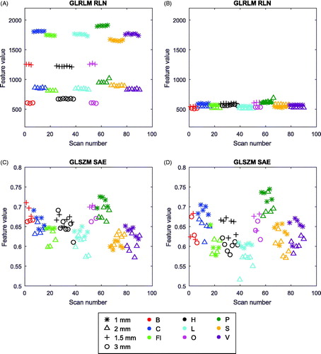
The feature ‘First order statistics (Stats) – Energy’ had the highest rank and thus showed the highest dependency on slice thickness and ‘GLRLM – Run Length Nonuniformity (RLN)’ the second highest dependency (Supplementary Material B). The feature ‘GLSZM – Small Area Emphasis (SAE)’ was least dependent on slice thickness and was ranked last. In further analyses in this study, we focused on the features ‘GLRLM – RLN’ and ‘GLSZM – SAE’, since ‘Energy’ is independent of gray-level discretization by definition. Figure 1 shows that the feature values for ‘GLRLM – RLN’ for 1.5 mm and 3 mm were more similar after resampling, which was not the case for the ‘GLSZM – SAE’ feature values. The test-retest analysis demonstrated that the feature ‘GLRLM – RLN’ is a stable feature (CCC > 0.85 for all bin widths), whereas the feature ‘GLSZM – SAE’ is unstable (Supplementary Material D).

Figure 1. Scatterplots of feature values for all scanners. Per scanner, the data is sorted from high to low exposure. Left: original data; Right: after resampling; Top: ‘GLRLM–RLN’, highest slice thickness dependency; Bottom: ‘GLSZM – SAE’, lowest slice thickness dependency.

For the feature ‘GLRLM – RLN’ the cubic, linear and nearest neighbor resampling method resulted in very similar feature ranges after resampling (Figure 2). For ‘GLSZM – SAE’, however, the nearest neighbor method resulted in a very wide range. When comparing the three resampling methods for all features tested (n = 114), for 34 (30%) features cubic interpolation resulted in the narrowest feature range, for 55 (48%) features this applied to linear interpolation, and the remaining 25 (22%) features had the narrowest feature range after nearest neighbor interpolation. Nearest neighborhood interpolation had the widest range for the majority (61%) of the features. For the feature that showed the highest dependency on slice thickness, ‘Stats – Energy’, feature values over all scans ranged from 6.3×10⁸ to 1.9×10⁹ (median 1.2×10⁹), which reduced to a range from 5.5×10⁸ to 6.9×10⁸ (median 6.1×10⁸) after resampling using cubic interpolation.

Figure 2. Bar plots of the spread of feature values of (A): ‘GLRLM–RLN’ and (B): ‘GLSZM – SAE’. Bars range from the minimum to the maximum observed value, and the vertical lines indicate the median. From top to bottom these bars are shown for all scans (n = 90), all scans with an exposure of 60 mA (n = 6), all scans with an exposure of 80 mA (n = 4), all scans with an increment of 1 mm (n = 34), 2 mm (n = 34) and 3 mm (n = 13) and all scans after resampling the images into 1 × 1 × 3 mm³ using cubic (n = 90), linear (n = 90) and nearest neighbor (n = 90) interpolation.

Figure 3 shows that the scans of the five different scanners had a similar median HU value: between 931 and 939 HU. When comparing the range in HU of those five scanners, scanner ‘P’ had a much wider range than the other four scanners (160–1564 compared to 437–1291). As shown in Figure 3 for the feature ‘GLCM cluster prominence’, this also affected radiomic feature values extracted from these images. The same histograms were made after resampling, which show a similar shape as before resampling (shown in Supplementary Material C).

Figure 3. HU distributions of the rubber insert scanned with a fixed CDTI of 5.43 mGy on five different Siemens and Philips scanners. From left to right and top to bottom [scanner - tube current]: ‘Fl-160mA’, ‘L-161mA’, ‘P-148mA’, ‘S-143mA’, and ‘V-162mA’. The scatterplot in the bottom right displays the observed values of the feature ‘GLCM cluster prominence’ over all scanners. The outlier in dark-green is scanner ‘P’.

Figure 4 shows that every normalized feature had another bin width dependency. Some features (e.g., ‘Energy’ and ‘Skewness’) were not dependent on bin width per definition. In terms of feature stability, when comparing 1.5 mm scans with 3 mm scans using an exposure of 60 mA, the total number of stable textural features hardly changed over the different bin widths (Figure 5). The median number of stable features was 49 (range 47–53). All CCC numbers for this comparison are shown in Supplementary Material D , where the features that were not stable in either the test-retest of ‘B-60mA-1.5mm’ or ‘B-60mA-3mm’ are also indicated. Also, when comparing an exposure of 60 mA with 80 mA on the same scanner, or scanner ‘B’ with ‘O’, no trend indicating a dependency on bin width could be observed. In this case, the median number of stable features was 66.5 (55–70) and 67.5 (56–72), respectively. Note that the total number of stable features was much lower when comparing different slice thicknesses.

Figure 4. Normalized feature values plotted against bin width. (A): GLCM features (n = 26), (B): GLDZM features (n = 16), (C): GLRLM features (n = 16), (D): GLSZM features (n = 16), (E): NGDLM features (n = 16), (F): NGTDM (n = 5) and first order statistics features (n = 2, dotted lines). The red dashed lines indicate GLRLM RLN and GLSZM SAE.

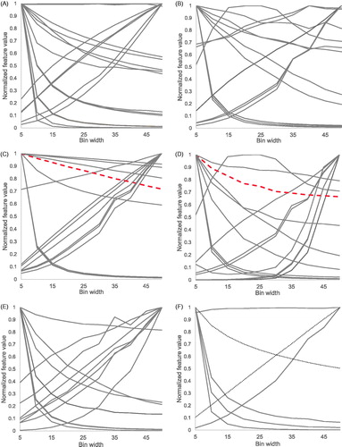
Figure 5. The total number of features with a CCC > 0.85 for each bin width when comparing (A) a slice thickness of 1.5 mm with 3 mm (exposure 60 mA, scanner ‘B’), (B) an exposure of 60 mA with 80 mA (slice thickness 3 mm, scanner ‘B’), or (C) scanner ‘B’ with ‘O’ using the same scan protocol (exposure 60 mA and slice thickness 3 mm). Test-retest figures are based on the minimal observed CCC in both test-retest sets that are compared.

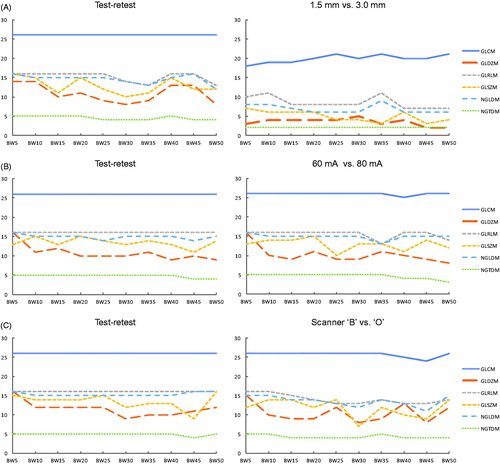
The images on the left side of Figure 5 show that approximately the same number of features were stable for the test-retest compared to the scans with different exposure or acquired from different scanners. On the other side, more features were stable in the test-retest setting than when slice thicknesses were different. The test-retest analysis of scan ‘B-60mA-3mm’ (bin width 25) shows that 5 out of 114 had a CCC below 0.85. When shifting the ROI downwards (ROI ‘6s324’ in Supplementary Material A), there were 8 features with CCC < 0.85, with 100% overlap compared to the test-retest. When shifting the delineation to the right (ROI ‘6s234’), 14 features were unstable, again with a 100% overlap.

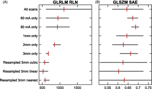
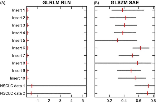
The range of feature values for all inserts was compared to the range in two independent datasets of NCSLC patients. As shown in Figure 6, the ‘GLRLM-RLN’ feature range observed in the phantom is very limited and substantially lower in comparison with the range observed in the clinical datasets, whereas the ‘GLSZM-SAE’ ranged in the same order of magnitude. The same plots for all features are available in Supplementary Material E.

Figure 6. Bar plots of the spread of feature values over all phantom inserts and two independent NSCLC datasets for (A): ‘GLRLM – RLN’ and (B): ‘GLSZM–SAE’. The bars indicate the minimum, median and maximum feature values. Scans were resampled to 1 × 1 × 3 mm³ voxels using cubic interpolation and a bin width of 25 HU was used.

Discussion

The aim of this study was to investigate the impact of different CT-scanners, slice thicknesses, exposures, gray-level discretization and resampling of voxel sizes on feature values and on their stability using a texture phantom. Moreover, we performed a test-retest analysis. In short, we could show that CT-scanner, slice thickness and gray-level discretization (i.e. bin width) influence feature values. A clear effect of exposure on feature values was not observed. Moreover, the stability of radiomic features is hardly influenced by bin width, i.e. for each bin width the variability across different settings is similar.

Scatterplots of feature values showed that the distribution of feature values is different for each CT-scanner. Since scans were acquired with the same range of CTDI values, this implies that the variability of feature values is affected by different scanners used in that particular study. The feature ‘GLSZM – SAE’, which has the lowest rank in terms of slice thickness dependency, appeared to be unstable in a test-retest analysis. In contrast the feature ‘GLRLM – RLN’ had a CCC above 0.85 for all test-retest scans, whereas the CCC was low in the comparison between 1.5 mm and 3 mm slice thickness (Supplementary Material D).

A comparable effect was observed in the HU histograms of five different scans that were acquired with the same CTDI of 5.43 mGy. The ‘Fl’, ‘L’, ‘V’, and ‘S’ scanners had comparable HU distributions within the rubber insert. However, even though the same radiation dose output of the CT-scanner and the same acquisition protocol was used, scanner ‘P’ resulted in a CT-image with a much wider range of HU. The histograms show the same pattern after resampling of the images was applied. The reason for the discrepancy of scanner ‘P’ is unknown, but it might be the result of an incorrect calibration of the scanner. So even with similar acquisition protocols, different scanner types within one dataset can influence radiomic feature values. Therefore, we recommend to take this into account when performing radiomic studies with multiple heterogeneous datasets, i.e., to perform a study specific test-retest analysis [16] to eliminate features that are not robust across different scanners.

We also showed that a large proportion of features is influenced by the slice thickness used for reconstruction. However, we could show that the variability in feature values decreased after resampling was performed. This is in line with Shafiq-ul-Hassan et al. [12], who showed that resampling reduced the feature variability from %COV >70% to %COV <30%. Therefore, we recommend to always perform resampling prior to any radiomic analysis. Despite the fact that resampling can greatly improve the robustness of radiomic features [12], we recommend to keep the voxel size as consistent as possible, since the variability in feature values is even lower when the voxel size is equal for all images included in the study. This should also be taken into account when comparing training and validation datasets that might be reconstructed into different voxel sizes, which could have increased the discrepancy between datasets in terms of distribution of radiomic feature values although resampling was applied. In our study the data was resampled to a voxel size of 1 × 1 × 3 mm³ using a cubic, linear and nearest neighbor interpolation, while in the study of Shafiq-ul-Hassan et al. [12] the data was resampled to a voxel size of 1 × 1 × 2 mm³ using a linear interpolation. Our results demonstrated that linear interpolation resulted in the narrowest feature value range for 48% of the features and cubic interpolation for 30% of the features, whereas nearest neighbor interpolation had the widest range for 61% of the features. Therefore, cubic or linear interpolation are preferred over nearest neighbor interpolation when resampling to 1 × 1 × 3 mm³ voxels.

Furthermore, we investigated the influence of exposure on the feature values, as tube current modulated CT-scans become more common. We only had data from a few scans per CT-scanner, which made it difficult to investigate the potential influence of exposure on radiomic feature values. For none of the features, we could see a clear relationship between feature value and the exposure. Mackin et al. [13] had quite a large range of exposure values for the different scanners, although the effect of exposure on feature values was not investigated, this might have influenced the scanner comparison results. In the future, the influence of exposure should be explored on a larger dataset.

Finally, we investigated the influence of the pre-processing step of ‘gray-level discretization’ on feature values and on their stability [18]. The main goal was to find an optimal bin width that could result in the highest reproducibility of radiomic features. Almost all features change in value when choosing another bin width for gray-level discretization. For a subset of features, a very small or very large bin width resulted in very different feature values across scans, whereas feature values are more similar with a bin size in the order of 25 (Figure 4). Although the feature values change for different bin widths, we were not able to show that the stability of radiomic features is greatly influenced by the choice of bin width (Figure 5 and Supplementary Material D). Our finding is the contrary of what Shafiq-ul-Hassan et al. described [12]. They found that only seven out of 51 features were reproducible independent of the gray-level discretization. Next to that, they found that seventeen out of 44 features showed a trend with varying number of gray-levels, which could be a linear, quadratic or cubic-type relation. Normalization of feature values by the number of gray-levels reduced the variation in feature values. However, these results imply that the choice of bin width could alter the prognostic value of a certain radiomic signature. The influence of gray-level discretization on the prognostic value of radiomic features has not yet been investigated and needs further research. Therefore, we cannot indicate a certain bin width as being most optimal, but we strongly recommend to be consistent and always clearly report which pre-processing steps have been used to improve the reproducibility and validation of radiomic studies [9].

The test-retest analysis we have performed shows that, even when not changing anything in between two subsequently acquired CT-scans, some radiomic features were not robust. When shifting the ROI within the same insert, even more features failed to reach a CCC above 0.85. The only reason for the instability of features in the test-retest setting could be the variability of scanner output, which is always present and cannot be avoided. Therefore, these features would be too unstable even when imaging protocols are completely standardized. We acknowledge that it is difficult to define a CCC threshold for eliminating the features, but we think that it is reasonable to exclude the non-stable radiomic features with CCC < 0.85 in future radiomic studies.

One of the limitations of this study is the ignorance of convolution kernel used during reconstruction. We considered the Philips ‘B’ kernel and the Siemens ‘B31s’ and ‘B31f’ as interchangeable, but this was not investigated. We also did not investigate the influence of iterative kernels or others commonly used in clinical practice, which might also affect the variability of radiomic features.

In this study, we investigated the influence of factors which we expected to have a major effect on radiomics. Nonetheless, other parameters influence image quality and therefore could have influenced the results. For example, scanners from different manufacturers have different possibilities for focal spot size and collimation width due to differences in technical design. These parameters do influence the image appearance: a smaller collimation width results in increased noise and a larger focal spot size results in decreased image quality (i.e. reduced sharpness). In the original design of the study we did not control for these parameters and the values were only traced back after the study was performed. In future studies, the influence of these parameters on radiomic features should be evaluated, and we recommend to report as much parameters as possible.

Furthermore, the potential influence of change in volume of the spherical region of interest was not investigated. Although all images were registered to the same reference scan which was used for delineations, this always leads to slightly different volumes. Whereas the spherical volume should consistently be 2.1 cm³, we noticed deviations in the order of 0.1 cm³. This could have influenced the results for radiomic features that are correlated to volume.

Another limitation of current and former studies [12,13] is the phantom itself. The squared shape makes the phantom prone to scatter artifacts around the edges. A new cylindrical version of the CCR phantom is therefore being produced and should be used in future CT-scanner variability studies.

In our study we compared the distribution of radiomic features values compared to two clinical NSCLC patient datasets. One possible explanation for the differences between the two patient datasets is that patient dataset 1 was acquired from multiple hospitals and dataset 2 from a single hospital, which might have resulted in a wider distribution of feature values for dataset 1. Furthermore, the distribution of feature values shows that not all inserts are very representative for clinical NSCLC datasets. Mackin et al. [13] already showed that the mean and standard deviation in HU of the CCR phantom is different than for patient data. The distribution of HUs in the rubber insert was most comparable to the distribution observed in the NSCLC datasets. However, radiomic features derived from any of the phantom inserts typically had a very limited range when compared to the clinical datasets, as well as a different median value. Inserts with more representative textures are, therefore, warranted for future phantom studies.

In conclusion, this study shows that feature values are influenced by CT-scanner, slice thickness and bin width, whereas the influence of exposure could not be shown. Moreover, the influence of bin width on feature stability was not clear, meaning that we could not indicate an optimal bin width. The test-retest analysis shows that some radiomic features are not robust in a strictly controlled setting: we recommend to exclude those in future radiomic studies. Moreover, we strongly recommend to always perform the pre-processing steps ‘resampling’ and ‘gray-level discretization’ for each radiomic study and to clearly report the settings that have been used to improve consistency and reproducibility of radiomic analyses.

Acknowledgments

The authors would like to acknowledge Dr. D. Mackin, Dr. L. Court and colleagues from The University of Texas, MD Anderson Cancer Center for the opportunity to use their CT-phantom in this study.

Disclosure statement

Ralph Leijenaar is a salaried employee of ptTheragnostic B.V., a company developing biomarkers and software to individualize radiotherapy treatment. Ralph Leijenaar and Philippe Lambin are co-inventors of several Radiomics patents.

Additional information

Funding

ERC10.13039/501100000781ERC-ADG-12-Hypoximmuno

Dutch Technology Foundation STW10.13039/5011000039586P14-19

EU4426

SME10.13039/10001067580–RAIL

EUROSTARSBD2Decide-PHC30-1508

ERC10.13039/100010663ERC-ADG-12-Hypoximmuno

Dutch Technology Foundation STW10.13039/5011000039586P14-19

EU4426

SME10.13039/10001067580–RAIL

EUROSTARSBD2Decide-PHC30-1508

The authors acknowledge financial support from ERC Advanced Grant (ERC-ADG-2015, no. 694812-Hypoximmuno). This research is also supported by the Dutch Technology Foundation STW (grant no. 10696 DuCAT & no. P14-19 Radiomics STRaTegy), which is the applied science division of NWO, and the Technology Programme of the Ministry of Economic Affairs. The authors also acknowledge financial support from the EU 7th framework program (ARTFORCE-no. 257144, REQUITE-no. 601826), SME Phase 2 (EU proposal 673780–RAIL), EUROSTARS (DART), the European Program H2020-2015-17 (BD2Decide-PHC30-689715 and ImmunoSABR-no. 733008), Kankeronderzoekfonds Limburg from the Health Foundation Limburg and the Dutch Cancer Society.

References

- Lambin P, Rios-Velazquez E, Leijenaar R, et al. Radiomics: extracting more information from medical images using advanced feature analysis. Eur J Cancer. 2012;48:441–446.
- Zhang Y, Oikonomou A, Wong A, et al. Radiomics-based prognosis analysis for non-small cell lung cancer. Sci Rep. 2017;7:46349.
- Leijenaar RTH, Carvalho S, Hoebers FJP, et al. External validation of a prognostic CT-based radiomic signature in oropharyngeal squamous cell carcinoma. Acta Oncol. 2015;54:1423–1429.
- Leijenaar RTH, Carvalho S, Velazquez ER, et al. Stability of FDG-PET Radiomics features: an integrated analysis of test-retest and inter-observer variability. Acta Oncol. 2013;52:1391–1397.
- Aerts HJWL, Velazquez ER, Leijenaar RTH, et al. Decoding tumour phenotype by noninvasive imaging using a quantitative radiomics approach. Nat Commun. 2014;5:4006.
- Coroller TP, Grossmann P, Hou Y, et al. CT-based radiomic signature predicts distant metastasis in lung adenocarcinoma. Radiother Oncol. 2015;114:345–350.
- Scrivener M, de Jong EEC, van Timmeren JE, et al. Radiomics applied to lung cancer: a review. Transl Cancer Res. 2016;5:398–409.
- Larue RTHM, Defraene G, De Ruysscher D, et al. Quantitative radiomics studies for tissue characterization: a review of technology and methodological procedures. Br J Radiol. 2017;90:20160665.
- Lambin P, Leijenaar RTH, Deist TM, et al. Radiomics: the bridge between medical imaging and personalized medicine. Nat Rev Clin Oncol. Forthcoming.
- Balagurunathan Y, Gu Y, Wang H, et al. Reproducibility and prognosis of quantitative features extracted from CT images. Transl Oncol. 2014;7:72–87.
- Lu L, Ehmke RC, Schwartz LH, et al. Assessing agreement between radiomic features computed for multiple CT imaging settings. PLoS One. 2016;11:e0166550.
- Shafiq-ul-Hassan M, Zhang GG, Latifi K, et al. Intrinsic dependencies of CT radiomic features on voxel size and number of gray levels. Med Phys. 2017;44:1050–1062.
- Mackin D, Fave X, Zhang L, et al. Measuring computed tomography scanner variability of radiomics features. Invest Radiol. 2015;50:757–765.
- van Timmeren JE, Leijenaar RTH, van Elmpt W, et al. Survival prediction of non-small cell lung cancer patients using radiomics analyses of cone-beam CT images. Radiother Oncol. 2017;123:363–369.
- Lin LI. A concordance correlation coefficient to evaluate reproducibility. Biometrics. 1989;45:255–268.
- van Timmeren JE, Leijenaar RTH, van Elmpt W, et al. Test-retest data for radiomics feature stability analysis: generalizable or study specific? Tomography. 2016;2:361–365.
- Zhao B, Tan Y, Tsai W-Y, et al. Reproducibility of radiomics for deciphering tumor phenotype with imaging. Sci Rep. 2016;6:23428.
- Leijenaar RTH, Nalbantov G, Carvalho S, et al. The effect of SUV discretization in quantitative FDG-PET Radiomics: the need for standardized methodology in tumor texture analysis. Sci Rep. 2015;5:11075.