Proton range shift analysis on brain pseudo-CT generated from T1 and T2 MR

Abstract

Background: In radiotherapy, MR imaging is only used because it has significantly better soft tissue contrast than CT, but it lacks electron density information needed for dose calculation. This work assesses the feasibility of using pseudo-CT (pCT) generated from T1w/T2w MR for proton treatment planning, where proton range comparisons are performed between standard CT and pCT.

Material and methods: MR and CT data from 14 glioblastoma patients were used in this study. The pCT was generated by using conversion libraries obtained from tissue segmentation and anatomical regioning of the T1w/T2w MR. For each patient, a plan consisting of three 18 Gy beams was designed on the pCT, for a total of 42 analyzed beams. The plan was then transferred onto the CT that represented the ground truth. Range shift (RS) between pCT and CT was computed at R₈₀ over 10 slices. The acceptance threshold for RS was according to clinical guidelines of two institutions. A γ-index test was also performed on the total dose for each patient.

Results: Mean absolute error and bias for the pCT were 124 ± 10 and −16 ± 26 Hounsfield Units (HU), respectively. The median and interquartile range of RS was 0.5 and 1.4 mm, with highest absolute value being 4.4 mm. Of the 42 beams, 40 showed RS less than the clinical range margin. The two beams with larger RS were both in the cranio-caudal direction and had segmentation errors due to the partial volume effect, leading to misassignment of the HU.

Conclusions: This study showed the feasibility of using T1w and T2w MRI to generate a pCT for proton therapy treatment, thus avoiding the use of a planning CT and allowing better target definition and possibilities for online adaptive therapies. Further improvements of the methodology are still required to improve the conversion from MRI intensities to HUs.

Background

Magnetic resonance (MR) imaging is often used for radiation therapy (RT) planning to contour the tumor and organs at risk (OAR) because it offers superior soft-tissue contrast compared to computed tomography (CT) imaging [1]. However, CT is preferred for dose calculation, because X-ray attenuation is easily converted into either electron density or relative stopping power for dose calculation purposes. To utilize the MR information for target definition, the MR is registered to the planning CT, but the registration process itself introduces systematic errors [2]. Hybrid MR/CT tomography scanners could minimize registration uncertainties [3], but the equipment is expensive and not widely available.

In recent years, several methods for converting MR into an artificial CT have been proposed and developed both in the context of radiation therapy [4] as well as for MR-based PET attenuation correction [5]. The artificial CT is commonly referred to as a pseudo-CT (pCT), and a standard method for its construction is to find a relation between MR intensities and Hounsfield Unit (HU). The advantages of using a pCT over MR-CT fusion are not limited at reducing the uncertainties inherent to image registration, but also at sparing the patient from the dose of a potentially unnecessary CT study. This is particularly true for: (1) pediatric patients, where dose upper limit is lower than for adults; (2) adaptive radiotherapy, where usually multiple X-ray based tomography (CT or Cone-Beam CT) are acquired.

Oborn et al. [6] discussed in his review the state of the art for both MR-guided photon and proton therapy, underlining how the latter will become relevant in the near future. The pCT workflow described in the review could also be suited for online plan adaptation.

Three approaches are commonly used for obtaining pCT from MR: (1) voxel-based, (2) atlas-based and (3) hybrid-based methods. The voxel-based method uses information from voxel intensities of MR to assign electron densities [7–9]. Either no or limited knowledge about anatomy is taken into account. Most of the procedures belonging to this group are machine-learning based, where either an algorithm is trained to predict HU values from MRI intensities [8] or a segmentation followed by bulk density assignment is used [10]. In atlas-based approaches, the patient’s MR is registered to an MR atlas, which contains prior correlation between image intensities and HU [11–13]. Hybrid-based conversion is a combination of the previous two methods [14–16]. Two comprehensive and up-to-date reviews of the methods proposed for radiotherapy planning have been written by Edmund et al. [4] and Johnstone et al. [17].

An issue common to all MR-to-CT conversion methodologies is the identification of tissues with short T2 relaxation time, such as cortical bone, which emit very little signal and can be misclassified as air. Ultra-short echo time (UTE) pulse sequences can mitigate this problem [18], but require a longer acquisition time. Thus, a pCT method that uses only standard T1/T2-weighted (T1w/T2w) sequences would be preferred if it accurately differentiates bone and air voxels, which is challenging as they do not contribute any signal to either T1w or T2w images.

While several studies analyzed and validated the employment of pCT for dosimetry in photon therapy [19,20], there is relatively little about the potential use of pCT for proton and ion therapy. Edmund et al. [10] and Rank et al. [21,22] proposed a voxel-based method for proton therapy using UTE sequences for brain and prostate respectively with a resulting mean average error (MAE) between CT and pCT corresponding to 130 HU (Edmund) and 140 HU (Rank); Zheng et al. [23] used UTE sequences as well, but generated a brain pCT by means of a Gaussian Mixture Model (GMM) (voxel-based method), obtaining a MAE of 147 HU. Koivula et al. [24] obtained a brain pCT by applying a voxel-based algorithm to T1w/T2w MR images, with the assumption that air/bone differentiation was not required because beams passing through air cavities are avoided in brain proton therapy planning, resulting in a MAE of 34 HU. Although this is generally true, prior to radiation many patients receive surgery, where a hole is drilled through the skull. Surgery can produce some air gaps between the skull and brain tissue that can potentially affect the final delivered proton dose.

Dosimetric evaluation conducted in the above-mentioned studies was mainly based on dose volume histogram (DVH) and γ-index analysis on the total dose. While these metrics alone are acceptable for photon therapy, they do not quantify range variations (which is a systematic error) for individual beams, which for proton therapy has a large dosimetric impact on the tumor and surrounding organs [25,28].

The goal of this work is to assess the feasibility of using T1w/T2w MR for treatment planning in proton therapy. We present and validate a new hybrid-based algorithm for the generation of pCT of the brain and skull. We evaluate this new algorithm via ‘leave-one-patient-out’ cross-validation method, which is a well-established method for a small set of samples. The novelties introduced in our study are:

1. obtaining pCT based on standard T1w/T2w MR without the need for UTE sequences for proton therapy planning;

2. using a cohort of patients with complex surgical holes and metal plates in the skull that significantly altered the local HU values and that are not easily viewed in the MR images;

3. assessing proton therapy plans with a beam-by-beam range shift analysis and comparing it with a γ-index test on the global dose to evaluate the sensitivities of the two approaches to HU re-assignment inaccuracies.

This work performs the first proton range uncertainty analysis of the use of pCT for proton therapy, following the method presented by Seco et al. [26]. In previous studies where pCT was used for proton therapy planning [10,21,22,24], the authors focused primarily on dose metrics such as (1) dose differences, (2) DVH or (3) γ-tests, which are not significantly sensitive to proton range shifts.

Material and methods

Patient data and method overview

Image data of 15 patients diagnosed with glioblastoma were employed in this study, although one patient had significant swelling between CT and MR and it was excluded from the dosimetric study. Images included, for each patient, T1w and T2w MR (MR_T1 and MR_T2, respectively) acquired post-contrast agent administration (Magnevist gadopentetate dimeglumine, Bayer HealthCare) and a CT scan of the head. All images were acquired after total or partial tumor resection.

MR images were obtained from a 3 Tesla MAGNETOM Trio (Siemens Healthcare GmbH, Erlangen, Germany), with a voxel size of 1 × 1 × 1 mm³ and reconstruction matrix of 256 × 256 × 256. Acquisition parameters were: TE = 1.64 ms, TR = 2530 ms, TI = 1200 ms for T1 (MPRAGE sequence) and TE = 475 ms, TR = 3200 ms for T2 (T2_SPACE sequence).

For CT scans a LightSpeed QX/i scanner (GE Healthcare, Chicago, IL, USA) was used, with the patient positioned for radiotherapy planning. Voxel size ranged from 0.49 × 0.49 × 2.5 mm³ to 0.67 × 0.67 × 2.5 mm³. CT and MR sequences were acquired on different days, with an interval between 10 and 20 days. Data processing and analysis workflow of the method included the following steps:

1. Image pre-processing,

2. Generation of conversion libraries to transform MR to pCT,

3. Proton treatment on pCT,

4. Comparisons between pCT and CT.

Image preprocessing

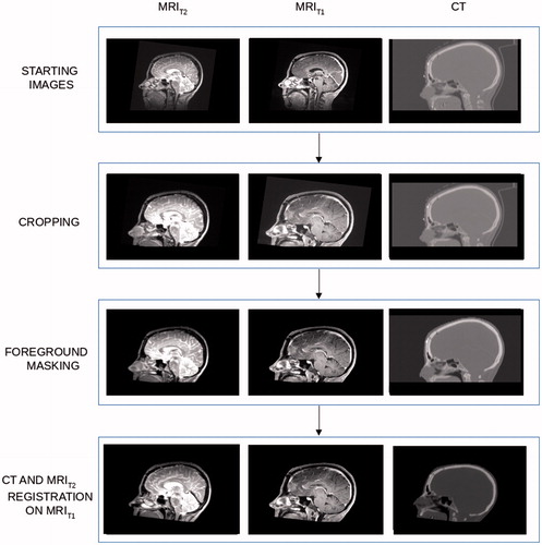
All image volumes were cropped at the level of the hard palate to exclude regions not of interest for this study (see Figure 1). The patient head was masked by using Plastimatch [27,28] with the background image intensities set to 0 and −1000 for MR and CT data, respectively. MR_T2 was rigidly registered to MR_T1 to compensate for slight patient head orientation between the two acquisitions. Finally, a rigid transformation was performed to register the CT to MR_T1. Image registrations were performed by Plastimatch setting Mattes Mutual Information (MMI) as optimizing metric with 2 × 2 × 2 voxel down-sampling. Before generating the pCT uniform normalization of the T1_w and T2_w images was performed using the white matter median value (see Appendix).

Figure 1. The lower part of the head was cropped because of the noise that would have altered the automatic segmentation process. After that, a foreground masking and a registration of the three modalities were performed in order to increase the accuracy of the pCT generation algorithm.

Pseudo-CT generation for proton planning

Voxel-based look-up-tables (LUTs) were derived to allow MR-intensities to be converted into pseudo HUs. In order to improve the accuracy of the conversion algorithm, voxels were classified based on (1) tissue type and (2) location in the head, where six tissue types and 11 anatomical regions within the brain were considered. Details about tissue segmentation and regioning are given in the Appendix. In total, 66 regio-segmental LUTs were built and they constituted a conversion library. Steps to generate each LUT were the following (see Figure 2):

Figure 2. Average HU value calculation: for each 10 × 10 T1_w/T2_w intensity bin, the average value is calculated, thus returning the HU value on the pCT for that patch.

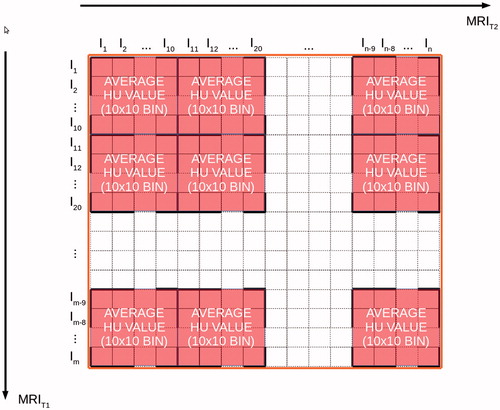
• for each voxel of the image volume, MR_T1 and MR_T2 intensities and real HU values were available;

• LUTs were generated by binning the HU in matrixes of 10 × 10 MR intensity units;

• the average of the HU values in one matrix was set as the target pCT value for this bin of MR values.

For voxels classified as ‘air’ in any region, conversion libraries were neglected and the bulk value of −1000 HU was assigned. At intersections of different conversion regions interpolation between LUT outputs was applied. The generation of the conversion library required in average 276 ± 9 s and it was obtained from the data of all the patients available for the study by leaving one out as independent data set for testing. The leave-one-patient-out cross-validation method was used to assess how the results of the pCT algorithm will generalize to an independent data set. This cross-validation evaluation involved partitioning our data set of 15 patients into complementary subsets, producing the LUTs on one subset (called the training set, which had 14 patients), and validating the model on the other subset (called the testing set, which had one patient, independent from the previous subset). To assess the robustness, we preformed the cross-validation 15 times and combined the results over the rounds to estimate the predictive capacity of our pCT model. In this model, the training set is completely independent from the testing set.

The process was repeated for all the patient data, each time leaving out a different patient to be used as the single test case.

At intersections of different conversion regions, interpolation between the conversion maps was applied. After the conversion, the images were smoothed by applying 3 × 3 × 3 linear kernel filters multiple times. The values of the kernel were set to 0.01/d, where is the distance to the central kernel value (in voxel numbers). The central kernel value was then set to be 1.0 minus the sum of the other values of the matrix.

The kernel was convoluted seven times to all of the pseudo-CT leaving out the bone tissue. The smoothing parameters were empirically chosen. The algorithm was implemented in Matlab (Mathworks, Natick, Massachusetts, USA). Computation time measurements were performed on a machine with an Intel Core i5 4260U @1.4 GHz (two cores, four threads) and 4 GB RAM.

Proton plan

For analysis and validation purposes, pCT was rigidly registered in the CT space, where the patient was set-up in the radiotherapy position. Plastimatch was run for image registration consisting of one registration step with MMI used as the metric and voxel subsampling of (1, 1, 1). The output transformation was used to register the MR_T1 onto CT, to better localize the tumor during the planning stage. MimVista Maestro™ (MimVista software Inc, Cleveland, OH, USA) was used to draw contours on MR_T1 aligned to the CT. Patient skin and PTV were generated and exported to CMS XiO (Elekta AB, Stockholm, Sweden). Proton passive scattering plans were designed on each pCT using three beams: one vertical, along the cranio-caudal (CC) direction, and two coplanar, in the axial plane (AX1 and AX2). Each beam was planned to cover the PTV with D₉₈ (18 Gy nominal dose). Dose cube workspace voxel measured 2 × 2 × 2.5 mm. Each plan on pCT was copied on the corresponding CT.

Data analysis

Commonly used metrics, mean absolute error (MAE) and mean error (BIAS), were used to assess the quality of pCTs in comparison to real CTs (1)

(2)

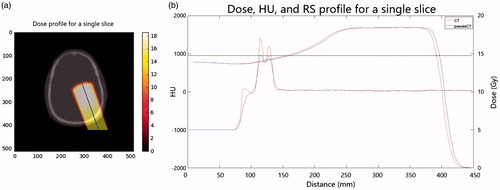
Only voxels which were inside the head volume were considered. Dose analysis was performed on the dose profile of 10 central slices of the dose cube in order to have the statistics to analyze the RS effect (one shift per slice). Range at 80% of maximum dose (R₈₀) was computed on the dose profile for each slice both for pCT and CT (Figure 3).

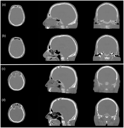
Figure 3. Visual comparison between pCT (a and c) and CT (b and d) for two representative cases. The zygomatic and frontal bones and the sinus cavities are most affected by wrong HU reassignment (c and d). The surgical holes present in the posterior left region of the skull (a and b) are satisfactorily reconstructed.

Range shift was defined as: (3)

RS relative to R_80CT (RRS) was computed as: (4)

Guidance on an acceptable level of RS came from range uncertainty criteria currently used in clinical applications at the Massachusetts General Hospital (MGH) and University of Florida Proton Therapy Institute (HPTI) [29]:

1. RS <3.5% R80CT +1 mm(MGH)

2. RS <2.5% R80CT +1.5 mm(HPTI)

A total dose assessment was performed using the 3D γ-index to compare the dose distribution (pCT vs. CT) within the PTV in the 10 slices selected for RS analysis. Plastimatch was used to perform the test. Distance to agreement (DTA) and dose difference (DD) criteria were 2 mm and 2%, respectively. Since the voxel dimension for the dose cube was 2 × 2 × 2.5 mm, a resample to a 2 × 2 × 2 mm was performed to allow the cube to be in the window of the γ-index test. The γ-index passing rate was set to 90%, as suggested by Mackin et al. in a proton therapy quality assurance study [30]. Dose Volume Histograms (DVHs) were computed within the PTV. In order to consider also an area around the tumor, DVH were calculated in 2-cm region surrounding the PTV, and this was assumed as organ at risk OAR.

Results

Quality estimation of the pCT

The pCT generation required in average 205 ± 8 s, and exhibited mean ± standard deviation of 124 ± 10 HU and −16 ± 26 HU for MAE and BIAS, respectively. pCT generally showed a good quality in the region of the calvaria, even in the presence of holes and metal inserts, and the cerebrum. Worse results were obtained for the facial region, especially in the paranasal sinus cavities, where air was mismatched with bone. A qualitative comparison between pCT and CT, emphasizing bony structures, is shown in Figure 4.

Figure 4. The dose profile is evaluated on a central line along the slices of the dose volume (a). For the same slice it the dose distribution and HU values for both pCT and CT along the beam line are plotted (b).

Evaluation of proton range shift

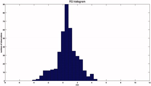
Figure 5 shows the signed RS distribution. The median and interquartile range of RS were 0.5 and 1.4 mm, with a minimum–maximum range of −3.9 to 4.4 mm.

Figure 5. Frequency distribution of the signed RS for all patients, in which the normal distribution of the RS can be observed. Example of dose profile with R₈₀ for pCT and CT, and the relative RS.

Table 1 shows, for every patient and every beam, the RRS on each of the 10 slices included in the analysis. Numbers highlighted in bold indicate the presence of metal along the path. Similarly, numbers highlighted in italic indicate the presence of air in the skull due to a surgical hole. In general, no correlation between RS magnitude and presence of air or metal was found. In total, 40 out of 42 beams showed RS of less than the clinically applied range margins. Both beams with larger RS were along the CC direction, where spatial resolution was poorer. Table 1 also reports the γ-index results, showing that dose coverage at 2 mm, 2% was always within the 90% acceptance threshold, min and max being 94% and 100%, respectively. The DVHs of PTV and OAR are reported in Figure 6 for patients 1, 2, 11 and 14, for planned total dose (56 Gy). These cases represent the worst situation according to RRS (patients 1 and 14) and total dose (patients 2 and 11). The difference between DVH values for CT and pCT for 95% of the total PTV volume was very small for all patients (about 0.5 Gy in the worst case, patient 11) indicating that the DVH is very little sensitive to range shifts per beam. In a normal proton therapy clinic CC beams for patients 1 and 14 would not have been used for treatment since they failed the RS assessment, while they yield practically equal DVH curves between CT and pCT.

Figure 6. DVH of the total dose delivered to the PTV and OAR (consisting of a 2-cm region surrounding the outside of the PTV) for patients 1, 2, 11 and 14. Blue lines are for pCT and red for CT.

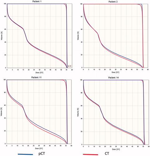
Table 1. Relative range shift, range shift test and γ-index test for each patient.

												RS test
						Relative range shift								γ–index test
Patient	Beam	Slice 01	Slice 02	Slice 03	Slice 04	Slice 05	Slice 06	Slice 07	Slice 08	Slice 09	Slice 10	MGH	HTPI	2%/2 mm
	AX1	0.40	0.46	0.53	0.32	0.27	0.52	0.47	0.55	0.25	0.18	√	√
1	AX2	0.95	0.60	0.54	0.91	0.49	0.69	0.80	0.69	0.51	0.40	√	√	96.97
	CC	5.71	6.30	7.16	6.79	6.30	5.71	7.61	8.90	7.49	5.64	x	x
	AX1	6.11	4.86	4.93	5.17	5.21	6.14	6.40	5.49	3.38	1.81	√	√
2	AX2	2.75	1.78	1.30	1.30	1.84	2.19	1.23	1.27	1.03	1.67	√	√	94.09
	CC	2.13	2.17	1.88	2.04	1.95	1.97	2.06	2.28	2.22	2.34	√	√
	AX1	2.66	2.18	1.98	1.60	2.32	2.24	2.30	2.80	2.80	2.89	√	√
3	AX2	3.15	2.97	3.00	2.98	3.04	2.81	2.72	2.69	2.80	2.88	√	√	99.39
	CC	1.09	1.44	0.98	1.04	0.95	0.77	0.88	1.09	1.11	0.72	√	√
	AX1	1.63	1.98	1.96	2.03	2.04	2.36	3.37	4.59	3.46	3.80	√	√
4	AX2	−0.66	−0.68	−0.61	−0.62	−0.57	−0.62	−0.96	−1.77	−2.27	−2.37	√	√	99.81
	CC	0.72	−0.67	−1.44	−2.73	−3.80	−5.54	−5.93	−4.75	−1.85	−0.30	√	√
	AX1	−0.35	−0.76	−0.71	−1.02	−0.95	−1.00	−1.18	−1.47	−1.42	−1.20	√	√
5	AX2	2.28	0.63	−2.92	−2.81	−1.42	−1.21	−0.19	0.11	0.23	0.24	√	√	99.11
	CC	3.56	3.67	3.88	4.04	4.07	4.02	3.64	2.48	1.04	0.73	√	√
	AX1	−0.19	0.04	0.31	0.36	0.37	0.41	0.41	0.60	0.49	1.37	√	√
6	AX2	0.69	0.73	0.71	0.81	0.91	0.83	0.69	0.57	0.65	0.77	√	√	100
	CC	0.03	0.29	0.36	0.28	0.15	0.10	0.05	0.01	0.00	0.07	√	√
	AX1	1.67	1.60	1.56	1.41	1.35	1.62	1.63	1.34	1.51	1.23	√	√
7	AX2	−0.03	−0.43	−0.93	−0.99	−1.16	−0.73	−0.66	−0.40	−0.63	−0.94	√	√	99.98
	CC	0.18	0.27	0.33	0.27	0.30	0.38	0.55	0.57	0.43	0.35	√	√
	AX1	1.36	1.24	1.23	1.20	1.29	1.29	1.09	1.57	1.07	1.96	√	√
8	AX2	1.06	0.66	0.63	0.77	0.75	0.75	0.97	1.19	1.12	0.98	√	√	100
	CC	1.44	0.54	−0.61	−0.62	0.04	0.83	1.17	1.74	2.75	2.97	√	√
	AX1	−0.69	−0.78	−0.46	−0.42	−0.52	−0.54	−0.50	−0.42	−0.30	−0.21	√	√
9	AX2	1.53	1.42	1.22	1.26	1.44	1.41	1.39	1.48	1.35	1.53	√	√	100
	CC	0.12	0.28	0.23	0.32	0.61	0.78	0.45	0.18	−0.10	−0.34	√	√
	AX1	1.04	2.51	0.88	0.80	0.58	0.90	0.55	0.48	0.64	0.49	√	√
10	AX2	0.74	0.60	0.97	1.11	1.21	0.84	0.83	2.24	1.89	1.52	√	√	100
	CC	−1.81	−1.83	−1.98	−1.52	−1.74	−1.92	−2.00	−2.14	−2.16	−1.55	√	√
	AX1	2.13	3.32	3.96	3.94	4.38	3.57	3.75	4.14	3.99	4.25	√	√
11	AX2	3.26	2.59	1.97	2.61	1.62	1.73	1.83	1.76	1.73	1.82	√	√	96.61
	CC	3.48	3.29	3.24	3.27	3.33	3.34	3.82	3.85	4.12	3.98	√	√
	AX1	−2.37	−2.36	−2.34	−2.17	−2.44	−2.39	−2.20	−2.36	−2.63	−2.49	√	√
12	AX2	−0.25	−0.32	−0.16	−0.08	−0.04	0.00	−0.04	−0.26	−0.64	−1.02	√	√	100
	CC	0.51	0.54	0.49	0.42	0.52	0.82	0.83	1.03	0.93	0.98	√	√
	AX1	−5.95	−2.33	−2.05	−2.21	−5.25	−2.27	−2.44	−3.37	−3.55	−3.20	√	√
13	AX2	1.16	1.05	0.60	0.58	0.72	0.77	1.05	1.00	2.08	0.82	√	√	100
	CC	−4.12	−4.33	−4.18	−0.94	−3.83	−3.78	−3.97	−4.38	−4.24	−4.28	√	√
	AX1	2.67	2.46	2.71	3.18	3.29	3.27	3.15	3.05	3.52	4.75	√	√
14	AX2	1.42	1.65	4.95	1.13	1.13	1.45	1.88	2.32	1.56	5.77	√	√	99.64
	CC	7.84	8.01	9.42	10.5	6.42	−0.25	−2.88	−1.16	0.41	3.27	x	x

Italic and bold cells represent presence, along the beam, of air and metal, respectively.

Discussion

With the widespread introduction of in-room MRI technology by ELEKTA (Elekta AB, Stockholm, Sweden) [31] and Viewray (ViewRay Inc., Cleveland, OH, USA) [32] for photon therapy, MRI offers the possibility of real-time radiotherapy treatment adaption for moving tumors. In order to perform real-time adaption of a radiotherapy treatment, electron density or stopping powers must be inferred from MR-images in real-time. In the present study, we investigate the feasibility and accuracy of using MRI to estimate proton-stopping powers needed for proton planning. At the moment, in-room online MR adaptive therapy is only commercially available for photon therapy, but on-going research is investigating how to combine MRI and protons for in-room real-time adaptive therapy [6]. This study presents a method of using MR for intracranial proton planning by converting MR intensities to HU values, which may be used for simulation or online adaptive therapy; especially the latter application could benefit from the use of pCT in order to minimize the patient radiation exposure and CT-MRI registration errors.

The strength of our method is that the pCTs are generated from MR_T1/MR_T2 MRI, which are standard imaging protocols in clinical practice. Even if specific sequences, like UTE, can be used to visualize the bone, they are not clinically widespread. The patient cohort investigated included air cavities and metal clips and plates in the skull from prior surgery. This made the assessment particularly challenging, allowing the dosimetric evaluation of treatment beams passing through heterogeneous tissues. In this situation, a fine conversion of MR to CT is preferred to bulk density override, as demonstrated in Koivula et al. [24].

The time to generate the conversion library required in average 276 ± 9 s, while the online pCT generation required 205 ± 8 s. This timing could make it possible to include the conversion procedure in to the clinical workflow.

It is worth noticing, however, that the hardware, used for the generation of both the libraries and the pCTs, was not very powerful. A more performing hardware, along with an implementation in a different coding language, could considerably lower the computational time.

MAE and BIAS metrics were used to quantify the differences between the reassigned HU values (pCT) and original HU values (control CT). Values are consistent with others presented in the literature [1,10,12]. Compared to the neurocranium, the viscerocranium posed a more demanding segmentation problem with less accurate air/bone separation, especially in the nasal region and in the sinus. Consequently, the accuracy of the pCT in these areas was compromised. Additionally, the pCT had lower quality in the caudal part of the images. A worse registration due to different cervical postures in the CT and MR, and lower MR image quality (lower SNR and loss of signal homogeneity) in those cervical parts are probable causes for the decreased quality. Since this study focused on the delivery of dose to the cerebral part of the brain of the patients, and radiation beams were not directed through the problematic parts of the generated pseudo-CTs, the obtained images were well suited for our experiment.

The regioning step in the pseudo-CT generation helps to increase the quality of the pseudo-CTs by separating the pseudo-CT derivation for different regions. Thus, for example errors in the segmentation of the viscerocranium will not compromise the pseudo-CT quality in the neurocranium. Also, it enables the algorithm to account for different tissue configurations at different anatomical sites.

The dose assessment was conducted by evaluating, for each beam, the RS between pCT and the corresponding original CT. A normal distribution of RS with positive mean was observed (Figure 5), indicating an overall underestimation of HU values. However, according to the clinical guidelines of two proton therapy centers, only two beams out of 42 presented a RS larger than the clinical range uncertainty margins. The two beams with larger RS (patients 1 and 14) occurred along the CC direction and were due to local misassignment of bone HU values, probably because of partial volume effects. Also, large delays between image acquisitions for the same patients led in some cases to visible differences in the skin, consequently affecting the range and the Bragg’s peak.

The presence of metal and surgical cavity air did not degrade the effectiveness of the pCT generation method. Metal was not present in either the tissue maps or in the anatomical regions of the conversion library, and the reassignment process recognized it as a high-density bone. The dosimetric assessment showed that, when the beam crosses the voxels that are supposed to be metal, even if a local difference in the HU values is evident, the resulting effect on the dose distribution is negligible.

Moreover, it is important to emphasize how an analysis performed on the whole dose, for instance by using the γ-index, can be inappropriate in proton therapy plan evaluation, where the range is the most crucial factor. In fact, according to γ-index on total dose, all plans included in this study would be considered acceptable while range errors for specific beams would have been hidden.

Finally, we would like to understand the feasibility of the presented approach in a clinical scenario. In our analysis, we found the main problems in HU misassignment and consequent range errors came from partial volume effects (especially in the CC direction because of the slice thickness) and, partly, from the inaccuracies of rigid registration. The MR and CT included in this study were not originally acquired for the purpose of this work. The patient head was positioned differently in the two acquisitions, and the time interval of up to 15 days led to anatomical differences. Moreover, the presence of contrast agent used to highlight the tumor changed the intensity of the voxels of the brain, altering the outcome of the segmentation in some cases. For a clinical protocol it would be preferred to set up the patient on the MR bed in the therapy position and acquire at least one sequence before the contrast injection.

One limitation is that, in order to transfer the method to other machines and MRI-sequences, a new library data with triplets of (MR_T1, MR_T2, CT) intensities from a set of patients have to be used and the parameters of the algorithm have to be adjusted to optimize performance on a new MRI-scanner.

Further studies are still required to improve the model in terms of minimization of MAE, BIAS and RS values and the applicability to other anatomic sites, like the prostate.

Finally, we are aware of the fact that the study involved a relatively low number of patients. This is due to the difficulties in obtaining a large number of CT/MRI pairs of patients. We are currently working in enlarging our database. However, our work provides a proof of principle for range shift analysis on pCT generated from MRI.

Conclusions

This study investigated the feasibility of using pCT, derived from standard T1 and T2 weighted MRI only, for proton therapy treatment planning in brain. The method achieved acceptable results in the presence of metal and air cavities, as shown by a beam-by-beam analysis of the proton range shift. However, further studies are still required to improve the model in terms of minimization of MAE, BIAS and RS values and the applicability to other anatomic sites, like the prostate.

Disclosure statement

No potential conflict of interest was reported by the authors.

Appendix

MRI intensity normalization

The MRI images in this study were tissue normalized, but no non-uniformal normalization (bias correction) was performed. The images were normalized, referring to the white matter median value, by the following steps.

1. The median intensity value of white matter voxels was calculated for each patient for MR_T1 and MR_T2 (The median values were around 750 and 150 for the MR_T1 the MR_T2, respectively).

2. 1500 and 300 were set as target intensity values for the median of white matter for MR_T1s and MR_T2s, respectively.

3. The normalization factors and were determined for all patients from the target median values (1500, 300) and the median white matter values and , (i is the index of the patients) (6) (7)

   with i being the index of the patient.

4. For each patient, MR_T1 and MR_T2MRIs were multiplied by their respective normalization factors, such that all the white matter median values for MR_T1 and MR_T2 were 1500 and 300, respectively.

Regioning and segmentation

The segmentation and regioning steps were essential to the pseudo-CT generation algorithm, as they allowed to transfer T1w and T2w MRI intensities to pseudo-HU in a regio-segmental specific way. The mapping from MRI intensities to CT HU is not unique, since same MRI intensity values can correspond to different HU values (a clear example is given by the fact that bone and air exhibit the same MRI intensity values, close to zero, in standard protocol MRIs). In order to overcome this problem, a tissue segmentation, prior to the pseudo-CT generation, was performed. Six tissues were labeled: gray matter, white matter, cerebro-spinal fluid, bone, skin and air.

MARS (Morphologically and Anatomically accuRate Segmentation) toolbox [33], an extension of SPM8 [34], was used for tissue segmentation. The voxel classification scheme was based on a Gaussian Mixture Model fit of MR data with anatomical prior from the atlas and morphological constraints on voxel neighbors using Markov random fields. Both MR_T1 and MR_T2 images were used as input to MARS. The output was six probability masks (V_p), that were converted in six binary tissue segmentation mask volumes (V_s) according to the following equation:

(8) where v_s and v_p are voxels in position (i, j, k) for V_s and V_p, respectively and t and z represent the six tissue classes.

One of the aims of the segmentation step was to differentiate air cavities in the cranial bone from the one in the nasal cavities: while cavities in the cranial bone like the frontal or maxillary sinuses were detected by the segmentation algorithm, the distinction of air and bone in the nasal cavity proved to be more inaccurate. Another important matter was the density of the bone: in some regions of the head, like the skull cap, there are normally no air cavities, and the problem of distinction between air and bone is not present, but as bone exhibits a low MRI intensity, there is also very little information in the MRI-data about its density. The HU values of bone can range from 500 to 1500 HU and the structure of bone can be very different depending on the anatomic region (cancellous vs. cortical bone). So, by adding a second step in the pre-processing, the regioning, it was possible to differentiate the conversion from MRI to HU values for different regions with different bone types (for example in the nasal cavity vs. the back of the head), thus reducing the degeneration of the mapping from MRI to pCT and improving the quality of the pseudo-CT values.

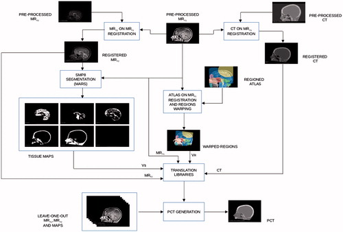
Regioning was accomplished by delineating 11 anatomical regions on a MR atlas [35] and obtaining a label map V_R. The 11 regions were the frontal sinus, nasal region, eyes, back of the head, teeth, middle cranial fossa, posterior cranial fossa, upper neck, anterior brainstem, remaining parts of the cranium and remaining parts of the image. Region labels were then transferred to each patient image volume by a 12-DOF (degrees-of-freedom) affine registration with Plastimatch of the atlas onto the MR_T1, since a perfect matching of patient and atlas was not necessary for this step. Figure 7 shows the whole workflow of the two processes.

Figure 7. Flow chart for the generation of the conversion libraries.

To further improve the quality of the generated LUTs, voxels from the edges of the segments were removed by eroding the segments by cuboidal kernel. This step was performed to exclude voxels with HU-values made up from different tissue types, due to partial volume effects or inaccurate segmentation. The erosion was performed by convolution of a 3 × 3 × 3 cuboidal kernel containing only ones with the binary segment volumes. If the convolution result was smaller than 27, the voxel was set to 0, otherwise to 1. The eroded segments were only used for the selection of voxels for the generation of the regio-segmental specific LUTs. For the pseudo-CT generation process the full segments were used.

References

- Schmidt MA, Payne GS. Radiotherapy planning using MRI. Phys Med Biol. 2015;60:323–361.
- Dean CJ, Sykes JR, Cooper RA, et al. An evaluation of four CT-MRI co-registration techniques for radiotherapy treatment planning of prone rectal cancer patients. Br J Radiol. 2012;85:61–68.
- Djan I, Petrovic B, Erak M, et al. Radiotherapy treatment planning: benefits of CT-MR image registration and fusion in tumor volume delineation. Vojnosanit Pregl. 2013;70:735–739.
- Edmund JM, Nyholm T. A review of substitute CT generation for MRI-only radiation therapy. Radiat Oncol. 2017;12:28.
- Izquierdo-Garcia D, Catana C. MR imaging-guided attenuation correction of PET data in PET/MR imaging. PET Clin. 2016;11:129–149.
- Oborn BM, Dowdell S, Metcalfe PE. Future of medical physics: real-time MRI-guided proton therapy. Med Phys. 2017;26:05.
- Korhonen J, Kapanen M, Keyrilainen J, et al. A dual model HU conversion from MRI intensity values within and outside of bone segment for MRI-based radiotherapy treatment planning of prostate cancer. Med Phys. 2014;41:011704.
- Johansson A, Karlsson M, Nyholm T. CT substitute derived from MRI sequences with ultrashort echo time. Med Phys. 2011;38:2708–2714.
- Catana C, van der Kouwe A, Benner T, et al. Toward implementing an MRI-based PET attenuation–correction method for neurologic studies on the MR-PET brain prototype. J Nucl Med. 2010;51:1431–1438.
- Edmund JM, Kjer HM, Leemput KV, et al. A voxel-based investigation for MRI-only radiotherapy of the brain using ultra short echo times. Phys Med Biol. 2014;59:7501–7519.
- Sjolund J, Forsberg D, Andersson M, et al. Generating patient specific pseudo-CT of the head from MR using atlas-based regression. Bull Am Meteor Soc. 2015;60:825–839.
- Dowling JA, Lambert J, Parker J, et al. An atlas-based electron density mapping method for magnetic resonance imaging (MRI)-alone treatment planning and adaptive MRI-based prostate radiation therapy. Int J Radiat Oncol Biol Phys. 2012;83:E5–E11.
- Izquierdo-Garcia D, Hansen AE, Förster S, et al. An SPM8-based approach for attenuation correction combining segmentation and nonrigid template formation: application to simultaneous PET/MR brain imaging. J Nucl Med. 2014;55:1825–1830.
- Hofmann M, Pichler B, Scholkopf B, et al. Towards quantitative PET/MRI: a review of MR-based attenuation correction techniques. Eur J Nucl Med Mol Imaging. 2009;36:93–104.
- Wagenknecht G, Kaiser HJ, Mottaghy FM, et al. MRI for attenuation correction in PET: methods and challenges. Magn Reson Mater Phy. 2013;26:99–113.
- Chen KT, Izquierdo-Garcia D, Poynton CB. On the accuracy and reproducibility of a novel probabilistic atlas-based generation for calculation of head attenuation maps on integrated PET/MR scanners. Eur J Nucl Med Mol Imaging. 2017;44:398–407.
- Johnstone H, Wyatt JJ, Henry AM, et al. Systematic review of synthetic computed tomography generation methodologies for use in magnetic resonance imaging – only radiation therapy. Int J Radiat Oncol Biol Physi. 2018;100:199–217.
- Bae WC, Chen PC, Chung CB, et al. Quantitative ultrashort echo time (UTE) MRI of human cortical bone: correlation with porosity and biomechanical properties. J Bone Miner Res. 2012;4:848–857.
- Arabi H, Koutsovelis N, Rouzaud M, et al. Atlas-guided generation of pseudo-CT images for MRI-only and hybrid PET-MRI-guided radiotherapy treatment planning. Phys Med Biol. 2016; 61:6531–6552.
- Andreasen D, Van Leemput K, Hansen RH, et al. Patch-based generation of a pseudo CT from conventional MRI sequences for MRI-only radiotherapy of the brain. Med Phys. 2015;42:1596–1605.
- Rank CM, Hunemohr N, Nagel AM, et al. MRI-based simulation of treatment plans for ion radiotherapy in the brain region. Radiother Oncol. 2013;109:414–418.
- Rank CM, Tremmel C, Hunemohr N, et al. MRI-based treatment plan simulation and adaptation for ion radiotherapy using a classification-based approach. Radiat Oncol. 2013;8:51.
- Zheng W, Kim JP, Kadbi M, et al. Magnetic resonance-based automatic air segmentation for generation of synthetic computed tomography scans in the head region. Int J Radiat Oncol Biol Phys. 2015;93:497–506.
- Koivula L, Wee L, Korhonen Feasibility of MRI-only treatment planning for proton therapy in brain and prostate cancers: dose calculation accuracy in substitute CT images. Med Phys. 2016;43:4634–4642.
- Knopf AC, Lomax A. In vivo proton range verification: a review. Phys Med Biol. 2013;58:R131–R160.
- Seco J, Panahandeh HR, Westover K, et al. Treatment of non-small cell lung cancer patients with proton beam-based stereotactic body radiotherapy: dosimetric comparison with photon plans highlights importance of range uncertainty. Int J Radiat Oncol Biol Phys. 2012;83:354–361.
- Sharp G, Li R, Wolfgang J, et al. Plastimatch-an open source software suite for radiotherapy image processing. Proceedings of XVIth International Conference on the Use of Computers in Radiotherapy (ICCR). Amsterdam, Netherlands; 2010. p. 7.
- Shickleford J, Shusharina N, Verberg J, et al. Plastimatch 1.6: current capabilities and future directions. Proceedings of MICCAI 2012 Image-Guidance and Multimodal Dose Planning in Radiation Therapy Workshop. Nice, France 2012.
- Paganetti H. Range uncertainties in proton therapy and the role of Monte Carlo simulations. Phys Med Biol. 2012;57:R99–R117.
- Mackin D, Zhu XR, Poenisch F, et al. Spot-scanning proton therapy patient specific quality assurance: results from 309 treatment plans. Int J Particle Therapy. 2014;1:711–720.
- Raaymakers BW, Jürgenliemk-Schulz IM, Bol GH, et al. First patients treated with a 1.5 T MRI-Linac: clinical proof of concept of a high-precision, high-field MRI guided radiotherapy treatment. Phys Med Biol. 2017;62:23L41–23L50.
- Acharya S, Fischer-Valuck BW, Kashani R, et al. Online magnetic resonance image guided adaptive radiation therapy: first clinical applications. Int J Radiat Oncol Biol Phys. 94:394–403.
- Huang Y, Parra LC. Fully automated whole-head segmentation with improved smoothness and continuity, with theory reviewed. PLoS One. 2015;10:e0125477.
- Penny W, Friston K, Ashburner J, et al. Statistical Parametric Mapping: the analysis of functional brain images. 1st ed. Oxford (UK): Academic Press; 2006. p. 696.
- Halle M, Talos IF, Jakab M, et al. Multi-modality MRI-based Atlas of the brain. SPL 2017 Jan.